
Chapter 8
Infinite Impulse Response (IIR) Filters
Abstract
The chapter introduces the infinite impulse response (IIR) filter. Infinite impulse response (IIR) filters are based on analog filters, where the frequency response is defined by both poles and zeros. Finite impulse response filters, in contrast, only have zeros. The presence of poles in the IIR filter causes the impulse response to be infinitely long. Poles are generated using feedback, which can also cause numerical instability. Despite these complications, IIR filters can be useful because for an equivalent frequency response, IIR filters require far fewer multipliers to implement. The process of designing an IIR filter is to start with an analog filter, and then map into the digital sampled domain.
Keywords
Bilinear transform; Butterworth analog filter; Filters; Infinite impulse response; Laplace transform; Prewarping; Z-transform
This chapter discusses infinite impulse response (IIR) filters. The IIR filter is unfortunately a much more complex topic than the FIR filter, and due to its nonlinear behavior, it is very difficult to analyze. It is also more complex to implement, due to the feedback, though it typically does require far less multipliers than a FIR filter. This feedback can cause instability in IIR filters, and overflow or underflow can easily occur using fixed point numbers. For these reasons, IIR is used much less than finite impulse response (FIR) filters. On the plus side, since it is not commonly used, understanding IIR filters is not essential to the fundamental concepts of digital signal processing (DSP). The IIR filter design technique is usually considered a bit of a specialty in the DSP world, so do not feel that you need to master this topic.
All the popular IIR filter designs are based upon analog filter circuits. The nature of analog components—capacitor, inductors, and opamps tend to be naturally suited to recursive filter designs. By contrast, FIR filters are naturally implemented digitally. This chapter will introduction to IIR filters, and then focus primarily on how to convert an analog IIR filter into a sampled digital implementation.
Mathematics for IIR filters tends to be more daunting. If the math proves too much, please note that the discussion in the chapter is not necessary to continue onto the other topics in the remainder of this book. Plus, the chapter following on digital modulation is really interesting; you would not want to miss it.
Most digital IIR filter designs are derived from analog filter designs. As analog filters were around long before digital filters existed, this provides for many types of filters.
The basic design procedure will be to take an analog filter design, and convert it to a digital IIR filter implementation. Since we do not have time or space to go through analog filter fundamentals, some material presented here may be difficult for readers who do not have any familiarity with analog filter design techniques.
Now, enough of the disclaimers, and let us begin.
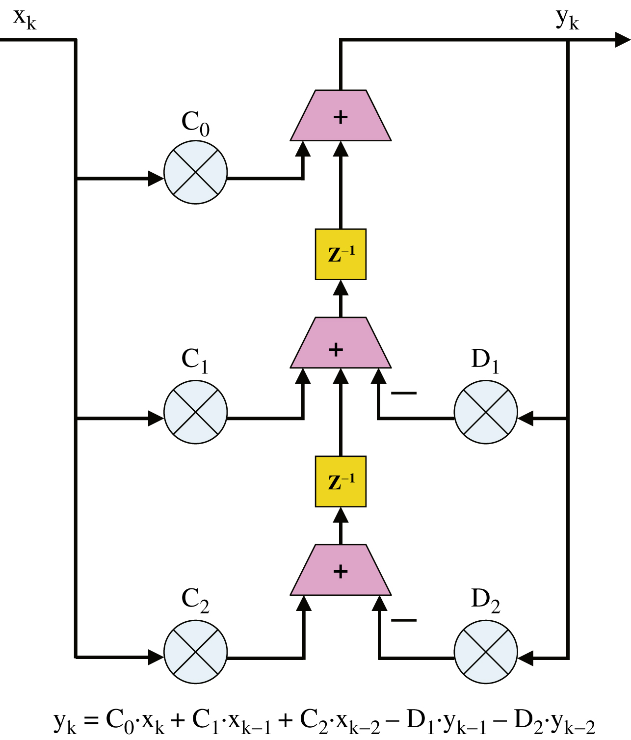
An IIR filter is basically an FIR filter with feedback added. The FIR filter takes a stream of input data and multiplies it by a series of coefficients to produce each output. The IIR filter also does this, but in addition, it feeds the output data stream back through another series of multipliers and coefficients. This structure is shown in the diagram below in Fig. 8.1.
This feedback eliminates many of the linear properties of the FIR filter and makes the IIR filter much more difficult to analyze. It can also create some undesired behavior, depending on the choice of coefficients, where the impulse response may have an infinite duration or even an infinite magnitude.
8.1. Infinite Impulse Response and Finite Impulse Response Filter Characteristic Comparison
Before we get too far into IIR filters, it is useful to compare IIR and FIR filters. Below is a summary of advantages and disadvantages of IIR and FIR digital filters.
• FIR filters have linear phase, meaning that no phase distortion of the signal occurs. IIR filters will always cause some phase distortion,1 so the phase as well as magnitude response needs to be considered by the filter designer.
• FIR filters can be designed with a specified amount of quantization noise (remember quantization from Numerical Representation chapter), which can be made as small as necessary. This is not the case with IIR filters.
• FIR filters can be implemented efficiently in multirate systems or systems that have decimation or interpolation steps.
• IIR filters are very sensitive to coefficient values and numerical precision, particularly in designs which require a sharp cutoff frequency response.
• IIR filters are more natural digital form to replace existing analog filters.
• An IIR filter can provide a much sharper cutoff frequency response compared to the same order (number of stages of multipliers) FIR filter. In other words, for sharp response in an FIR filter, more resources (multipliers and adders) are required than in IIR filter.
Based on this, one wonders why anyone would want to use IIR filters. Well, aside from the last bullet, which lists a key advantage of IIR filters, the reason is that IIR filters can best approximate the performance of many analog filter responses. Sometimes when a system with analog filtering is being upgraded to digital implementation, it is important to preserve its performance characteristics, especially in the phase domain. An example of this might be professional audio equipment.
Intuitively, the reason IIR filters can have a much more rapid frequency response is because their frequency response is determined by both “zeros” and “poles”. Zeros are caused by cancellations. Remember the FIR discussion, with coefficients of +1, −1, +1, −1, and so on? This filter causes cancellations at high frequencies, and this can be described as zero at a specific frequency. Filter response is determined by canceling various frequencies.
Poles, on the other hand, involve feedback and result in an effect similar to division by zero at specific frequencies. Actually, this is not exactly divided by exactly zero, as this would produce an infinite response, but the idea is to divide by a very small number at certain frequencies, which can produce a large output in the signal in that frequency region. Think of a rope representing frequency response. The poles would hold the rope up at specific points, and the zeros would be like a lead weight holding it to the ground at other points. This is analogous to how poles and zeros can act on the frequency response.
The additional flexibility of using poles with zeros, while resulting in some unstable filter responses, if not careful (imagine a pole which can provide very high, or even infinite gain), can also provide for more rapid changes in the frequency response. This makes IIR filters more sensitive and complicated than FIR filters.
In this introductory chapter, we will not try to explain the design of IIR filters using pole and zero placement. There are whole books on this topic and is too much for this introductory treatment here. Rather we will show how to take popular analog filter designs, with a defined pole and zero arrangement and thus frequency response, and convert to a digital implementation, as this is a more common task for a DSP system designer.
Even a basic understanding of IIR filters will require some mathematics. The reason is that analog filters are analyzed using something called the “Laplace transform.” Digital filters are analyzed using something called the “z-transform.” Because of their simplicity, we managed to avoid the z-transform when discussing FIR filters, but we will not have that option here. Please refer to the appendices at the end of book introducing Laplace and Z-transforms if these are new to you.
8.2. Bilinear Transform
The normal design procedure for IIR filters is to specify the filter response and design an analog filter using analog filter techniques (using Laplace transform). Alternately, you might be given an analog filter design, and be asked to convert it to a digital implementation. The analog filter design is based on the location of poles and zeros in the “s” plane. A digital filter response can be characterized by using z-transform. The equivalent pole and zero domain for digital filters is called the “z” plane. The idea is to map the “s” plane poles and zeros to the “z” plane. The mapping technique most often used between the “s” and “z” domains is called the bilinear transform. There are alternative techniques, but we will not cover these here. Further, only a rudimentary coverage will be attempted here, as the topics involved are fairly mathematical.
Again, please note that both the Laplace and z-transforms are reviewed in appendices at the end of this book. If you have not looked at these recently, you may want to spend a little time going through Laplace and Z-transform appendices.
We use ώ for the s-plane to distinguish between ω of the sampled domain z-plane. Similarly, we will define the frequency response of the analog filter as Hs and the frequency response of the digital filter as Hz.
In analog filter design, the frequency response of an analog filter is defined by setting s = jώ and evaluating for −∞ < ώ < ∞. This corresponds to the imaginary axis of the s-plane.
The frequency response of a digital filter is defined by setting z = ejω, and evaluating for −π < ω < π. This corresponds to the unit circle of the z-plane.
To go between these two domains, we need a mapping function from the s-plane to the z-plane. Then we can map the zeros and poles across the two domains.
This is performed by replacing s in the expression for Hs.
Let us go through an example of converting and analog filter to a digital IIR filter. There are a great many analog filter types. Here we will discuss only one, as analog filters are not the topic we want to focus on. A very common analog filter is the Butterworth filter. It has the characteristic of not having ripples in the passband or stopband.
We will be taking a third-order Butterworth analog filter and converting to an IIR digital filter using the bilinear transformation technique. Many analog filters are known simply by their pole and zero locations (since this is another way of defining frequency response). We can eliminate quite a bit of algebra by using the relationship above between s and z domains to come up with a relationship between poles and zeros in the s and z domains. These derivations are not discussed here, only the result is discussed.
The IIR digital filter will have poles and zeros at locations:
We will set the cutoff frequency of our third-order Butterworth filter to 100 Hz, or 628 radians/second (100·2·π). For a third-order Butterworth filter, the three pole locations in the s-plane are located at:
We will set our digital sampling frequency at 1000 samples per second, so T = 0.001. The s-domain poles will map to the following poles in the z-plane.
The Butterworth filter has three zeros located at infinity. These can be evaluated as:
Now that we have the poles and zeros on the z-plane, we can determine the z-transform of the digital IIR filter approximating the response of the analog Butterworth filter.
where M = number of zeros and N = number of poles. In our example, M = N = 3. With a bit of algebra, we can multiply this whole mess out, to get in the more familiar form.
In this form, we can pick off our coefficients needed to implement the IIR filter.
Multiplying the numerator and denominator components, we will get:
From inspection,

These C and D coefficients apply to the IIR filter structure depicted earlier in the chapter (although this is a third-order filter, the example diagram is second order).
8.3. Frequency Prewarping
We still have another point to consider. Our technique is to take the pole and zero locations (in the s-plane) of an analog filter, and to map them to pole and zero locations (in the z-plane) of an IIR digital filter.
The problem is that this relationship is not linear. For example, the y-axis of the s-plane, which is infinite in length, is mapped to the unit circle in the z-plane. This relationship is
This nonlinear mapping will cause filter response distortion, particularly at higher frequencies. A method to mitigate this is to prewarp the analog filter. The whole analog filter is not prewarped, instead key breakpoints in the analog filter response are prewarped. This will in essence stretch the analog filter in frequency, so that when it is compressed by the bilinear transform, the prewarped breakpoint(s) will be mapped correctly. This ensures that transition points between pass and stopband are accurately converted by the bilinear transform.
The table below shows the distortion cause by mapping between the s and z domains. For this table, we set T = 1. Note how this distortion or warping increases with frequency (Table 8.1).
Let us consider a simple example. We have an analog low-pass filter, with a 3 dB breakpoint at 100 Hz (3 dB breakpoint is the point in transition band where filter response is 3 dB lower than the passband response). We want to implement this filter with a digital IIR filter, which will have an Fs = 1000 Hz.
The digital breakpoint frequency should be (100/1000)·2π = 0.2·π. The warping will cause this breakpoint to occur at digital frequency 0.1938·π instead.
The analog filter breakpoint needs to be moved, or prewarped, to compensate for this.
Substituting into ώ (s-plane) = (2/T)·tan(ω/2), we find
We should design the analog filter with a 3 dB point at 103.4 Hz, rather than 100 Hz prior to converting to a digital IIR filter using the bilinear transform to map the pole/zero locations.
To illustrate the effect as the frequency rises, let us revise the problem to building a digital filter to replace an analog filter with a 3 dB breakpoint at 250 Hz. We will still use Fs = 1000 Hz.
The digital frequency of the breakpoint is ω = (250/1000)·2π = 0.5·π.
The analog frequency of the breakpoint needs to be moved from 250 Hz to prewarp the filter. The new analog filter breakpoint is found to be:
We can see that the importance of prewarping the analog filter prior to applying the bilinear transform as we move our breakpoint closer to the Nyquist frequency of the digital filter (in this example, equal to 500 Hz). If there are multiple transition points, they can all be prewarped, and the analog filter modified to meet these new transition points.
For those of you without much analog filter design experience, you may be wondering how to modify the analog filter, to find prewarped analog poles and zeros which will then be mapped to the digital domain. This is a valid question, but unfortunately is beyond the scope of this chapter. The focus of our discussion is how to learn the basics of converting an analog filter to a digital IIR filter. Since analog filter design a complex and mathematical subject, this just too much to try to cover here. However, as you might expect, there are software programs which can be used to perform analog filter design, and even convert these to a digital IIR design.
..................Content has been hidden....................
You can't read the all page of ebook, please click here login for view all page.