Search in book...
Toggle Font Controls
Create new playlist

Name your new playlist

Playlist description (optional)
Sign In

Email address

Password

Forgot Password?

or

Continue with Facebook

Continue with Google
Sign Up

Full Name

Email address

Confirm Email Address

Password

or

Continue with Facebook

Continue with Google

Chapter 13

Matrix Inversion

Abstract

Matrix processing is a heavily used technique in communications, radar, medical imaging, and many other applications. This is particularly prevalent in systems with many antennas and performing multiple input, multiple output (MIMO) processing. In 5G wireless, for example, QR decomposition (QRD) is used in both MIMO processing and amplifier digital predistortion adaptation. In radar, QRD is used in space–time adaptive processing (STAP) and can be used to extract signals well below the noise floor. This chapter has more math than most. These functions are usually already available as library functions for high performance CPUs, GPUs, and FPGAs.

Keywords

Cholesky decomposition; Determinate; Hermitian; Nonsingular; Orthogonal matrix; Orthonormal matrix; QR decomposition

Matrix processing is a heavily used technique in communications, radar, medical imaging, and many other applications. This is particularly prevalent in systems with many antennas and performing multiple input, multiple output (MIMO) processing. In 5G wireless, for example, QR decomposition (QRD) is used in both MIMO processing and amplifier digital predistortion adaptation. In radar, QRD is used in space–time adaptive processing (STAP) and can be used to extract signals well below the noise floor. The matrix sizes used are normally modest, but the throughput and processing requirements can be very high. This chapter has more math than most. Note, however, that these functions are usually already available for high performance CPUs, GPUs, and FPGAs.

Matrix inversion techniques, such as QR or Cholesky decomposition, typically involve very small and large numbers in the computation process, which requires a dynamic range that is impractical to support using fixed point numerical representation. Both are computationally intensive and grow in computational requirements by the third power of the matrix dimensions. A matrix of [1000 × 1000] has 1 million elements, and this is a nontrivial effort to find the inverse, assuming it exists.

13.1. Matrix Basics

A matrix is made up of vectors. These can be defined as column or row vectors, depending upon the context. For example, an [M × N] matrix can be defined as N column vectors, where each vector is of length M. This section covers basics of matrix multiplication.

The inverse of matrix is defined as

$A \cdot A^{- 1} = I,$ $A \cdot A^{- 1} = I,$

where A⁻¹ is the inverse of the matrix A.

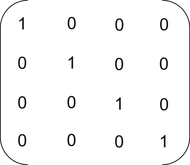
This simply means that a matrix multiplied by its inverse equals the identity matrix. The identity matrix is a matrix with diagonal elements all equal to 1, and every element off the diagonal equal to zero (Fig. 13.1).

Matrices have a property known as the determinate, which is a value that can be computed from the elements of the matrix. An invertible matrix is called nonsingular and has a nonzero determinate. When the determinate is zero, the matrix is singular and the inverse matrix does not exist. An “ill-conditioned” matrix has a determinate near zero. In practice, this will mean that computing the inverse will have some very small and/or very large numbers involved and will require a high degree of numerical accuracy.

Figure 13.1 Identity matrix (dimension = 3).

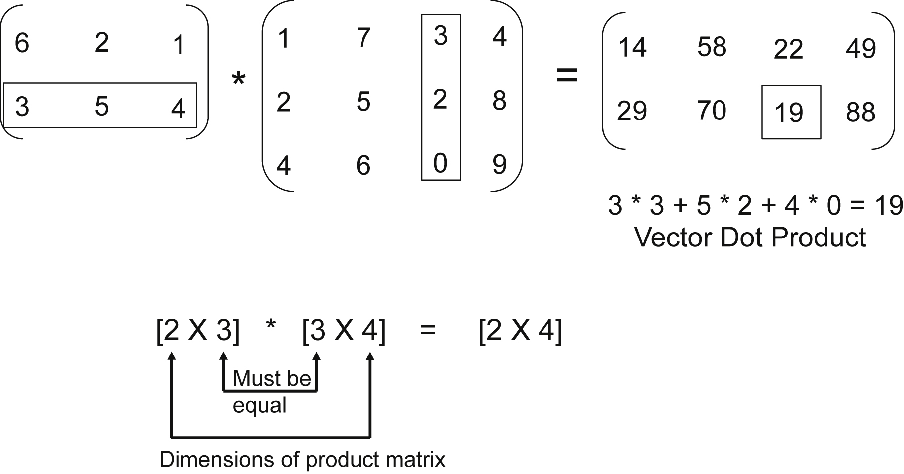
Matrix multiplication involves taking the dot product between two vectors to compute the each element of the resulting matrix. The dot product means taking two vectors, multiplying each pair of elements, and summing the products. The dot product of two vectors results in a scalar result (Fig. 13.2).

In order to multiply two matrices A · B = C, the number of columns in A must equal the number of rows in B. This is necessary, so when computing the dot product, the vector lengths will be equal. If A is an [N × M] matrix, then B must be an [M × P] matrix to perform the matrix multiplication and C will be of size [N × P]. In the example in Fig. 13.3, the matrix dimension of A is [2 × 3], B is [3 × 4], and C is [2 × 4]. The vector dot product is identified to compute output element C₂₃.

For an [N × N] matrix to be invertible, all of the column vectors need to be independent of each other (Fig. 13.4).

Using of a [3 × 3] matrix, we can imagine a three-dimensional space. Each column vector represents a vector starting from the origin and terminating at the point defined by the vector in the three-dimensional space. If each vector points in a different direction, then the vectors are independent of each other. If two vectors point in exactly the same direction (they may be of different lengths), then the vectors are dependent. If there is a 90-degree angle between two vectors, then they are not only independent but also orthogonal to each other. If all the vectors are 90 degrees with respect to each other (for example, the three axis vectors shown in Fig. 13.4), then the matrix is an orthogonal matrix.

Figure 13.4 Matrix composed of vectors in N-dimensional space.

Ill-conditioned matrices have two or more vectors that are close to colinear or nearly in the same direction. Because the vectors are very close to being dependent, this will be a matrix that will require a high degree of accuracy in determining the inverse.

13.2. Cholesky Decomposition

The Cholesky decomposition is used in the special case when A is a square, conjugate symmetric matrix. This makes the problem a lot simpler. Recall that a conjugate symmetric matrix is one where the element A_jk equals the element A_kj conjugated. This is shown as A_jk = A_kj∗. If A_jk is a real value (not complex), then A_jk = A_kj.

Note: A conjugate is then the complex value with the sign on the imaginary component reversed. For example, the conjugate of 5 + j12 = 5 − j12. And by definition, the diagonal elements must be real (not complex), since A_jj = A_jj∗, or more simply, only a real number can be equal to its conjugate.

The Cholesky decomposition floating point math operations per [N × N] matrix is generally estimated as:

$FLOPS = 4 N^{3} / 3$ $FLOPS = 4 N^{3} / 3$

However, the actual computational rate and efficiency depend on implementation details and the architecture details of the computing device used (CPU, FPGA, GPU, DSP…).

The problem statement is A · x = b, where A is an [N × N] complex symmetric matrix, x is an unknown complex [N × 1] vector, and b is a known complex [N × 1] vector. The solution is x = A⁻¹ · b, which requires the inversion of matrix A (Fig. 13.5). As directly computing the inverse of a large matrix is difficult, there is an alternate technique using a transform to make this problem easier and require less computations.

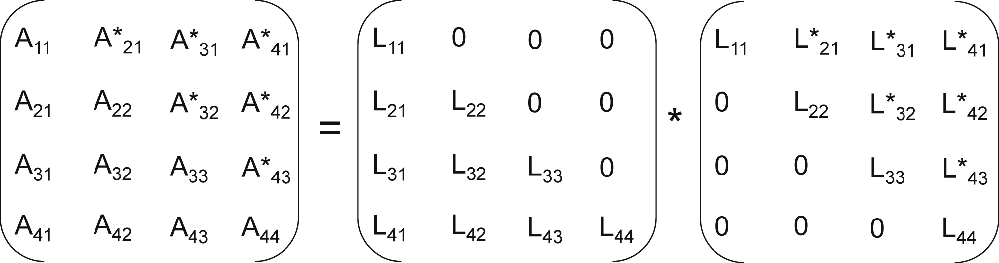
The Cholesky decomposition maps matrix A into the product of A = L · L^H where L is the lower triangular matrix and L^H is the transposed, complex conjugate or Hermitian, and therefore of upper triangular form (Fig. 13.6). This is true because of the special case of A being a square, conjugate symmetric matrix. The solution to find L requires square root and inverse square root operators. The great majority of the computations in Cholesky is to compute the matrix L, which is found to be expanding the vector dot product equations for each element L and solving recursively. Then the product L · L^H is substituted for A, and after which x is solved for using a substitution method. First the equations will be introduced, then an example of the [4 × 4] case will be shown to better illustrate.

(L′ is commonly used to indicate L^T or L^H if the matrix is complex)

Solving for the elements of

$A_{j j} = \sum_{k = 1}^{j} L_{j k} \cdot L_{k j}^{'}$ $A_{j j} = \sum_{k = 1}^{j} L_{j k} \cdot L_{k j}^{'}$

where j is the column index of the matrix

$A_{j j} = \sum_{k = 1}^{j} L_{j k} \cdot c o n j (L_{j k})$ $A_{j j} = \sum_{k = 1}^{j} L_{j k} \cdot c o n j (L_{j k})$

The first nonzero element, in each column, is a diagonal elements and can be found by

Diagonal Elements of L

$L_{j j} = \sqrt{A_{j j} - \sum_{k = 1}^{j - 1} L_{j k} \cdot c o n j (L_{j k})}$ $L_{j j} = \sqrt{A_{j j} - \sum_{k = 1}^{j - 1} L_{j k} \cdot c o n j (L_{j k})}$

(13.1)

In particular,

$L_{11} = \sqrt{A_{11}}$ $L_{11} = \sqrt{A_{11}}$

Similarly, the subsequent elements in the column are related as follows:

$A_{i j} = \sum_{k = 1}^{j} L_{i k} \cdot L_{k j}^{'}$ $A_{i j} = \sum_{k = 1}^{j} L_{i k} \cdot L_{k j}^{'}$

where i and j are the row and column indices of the matrix

$A_{i j} = \sum_{k = 1}^{j} L_{i k} \cdot c o n j (L_{j k})$ $A_{i j} = \sum_{k = 1}^{j} L_{i k} \cdot c o n j (L_{j k})$

where

L_{j k}

$L_{j k}$

is the transpose of

L_{k j}

$L_{k j}$

Off-diagonal elements of L

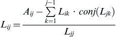$L_{i j} = \frac{A_{i j} - \sum_{k = 1}^{j - 1} L_{i k} \cdot c o n j (L_{j k})}{L_{j j}}$ $L_{i j} = \frac{A_{i j} - \sum_{k = 1}^{j - 1} L_{i k} \cdot c o n j (L_{j k})}{L_{j j}}$

(13.2)

By substituting for L_jj the full recursion can be seen

$L_{i j} = \frac{A_{i j} - \sum_{k = 1}^{j - 1} L_{i k} \cdot c o n j (L_{j k})}{\sqrt{A_{j j} - \sum_{k = 1}^{j - 1} L_{j k} \cdot c o n j (L_{j k})}}$ $L_{i j} = \frac{A_{i j} - \sum_{k = 1}^{j - 1} L_{i k} \cdot c o n j (L_{j k})}{\sqrt{A_{j j} - \sum_{k = 1}^{j - 1} L_{j k} \cdot c o n j (L_{j k})}}$

Eqs. (13.1) and (13.2) are the equations that will be used to find L_jj and L_ij. In solving for one element, a vector dot product proportional to its matrix size must calculated.

Although matrices A and L may be complex, the diagonal elements must be real by definition. Therefore, the square root is taken of a real number. The denominator of the divide function is also real.

Once that L is computed, perform the substitution for matrix A:

$A \cdot x = b \to L \cdot L^{H} \cdot x = b$ $A \cdot x = b \to L \cdot L^{H} \cdot x = b$

Next, we want to introduce an intermediate result, the vector y. The product of matrix L^H and vector x is defined as the vector y.

$y = L^{H} \cdot x \to L \cdot y = b$ $y = L^{H} \cdot x \to L \cdot y = b$

The vector y can be computed by a recursive substitution, called forward substitution, because it is done from top to bottom. For example, y₁ = b₁/L₁₁. Once y₁ is known, it is easy to solve for y₂ and so on.

To restate, L and L^H are known after the decomposition, and L · L^H · x = b. Then we define L^H · x = y and substitute. Then we are solving L · y = b. L is a lower triangular matrix, y and b are column vectors, and b is known. The values y_j can be found from top to bottom using forward substitution. The equations to find y is

Intermediate result y

$y_{j} = \frac{b_{j} - \sum_{k = 1}^{j - 1} y_{k} \cdot L_{j k}}{L_{j j}}$ $y_{j} = \frac{b_{j} - \sum_{k = 1}^{j - 1} y_{k} \cdot L_{j k}}{L_{j j}}$

(13.3)

Eq. (13.3) is almost the same as Eq. (13.2). If we treat b as an extension of A and y as an extension of L, the process of solving y is the same as solving L. The only difference is, in the multiply operation, the second operand is not conjugated (this consideration may be important for hardware implementation, allowing computational units to be shared).

After y is computed, x can be solved by backward substitution in L^H · x = y (Fig. 13.7). L^H is an upper triangular matrix, therefore, x has to be solved in reverse order—from bottom to top. That is why it is called backward substitution. Therefore, solving x is separate process from the Cholesky decomposition and forward substitution solver.

Figure 13.7 Solving for y and then for x.

In addition, y has to be completely known before solving x. The equation to solve x is shown below, where VS = N is the length of vectors x and y.

Desired result x

$x_{j} = \frac{y_{j} - \sum_{k = j + 1}^{V S} x_{k} \cdot L_{j k}^{'}}{L_{j j}^{'}}$ $x_{j} = \frac{y_{j} - \sum_{k = j + 1}^{V S} x_{k} \cdot L_{j k}^{'}}{L_{j j}^{'}}$

(13.4)

The algorithm steps and data dependencies are more easily illustrated using a small [4 × 4] matrix example.

13.3. 4 × 4 Cholesky Example

$\begin{matrix} A = [\begin{matrix} L_{11} & 0 & 0 & 0 \\ L_{21} & L_{22} & 0 & 0 \\ L_{31} & L_{32} & L_{33} & 0 \\ L_{41} & L_{42} & L_{43} & L_{44} \end{matrix}] [\begin{matrix} L_{11} & L_{21} & L_{31} & L_{41} \\ 0 & L_{22} & L_{32} & L_{42} \\ 0 & 0 & L_{33} & L_{43} \\ 0 & 0 & 0 & L_{44} \end{matrix}] \\ = [\begin{matrix} L_{11}^{2} & C o n j u g a t e S y m m e t r i c \\ L_{21} L_{11} & L_{21}^{2} + L_{22}^{2} \\ L_{31} L_{11} & L_{31} L_{21} + L_{32} L_{22} & L_{31}^{2} + L_{32}^{2} + L_{33}^{2} \\ L_{41} L_{11} & L_{41} L_{21} + L_{42} L_{22} & L_{41} L_{31} + L_{42} L_{32} + L_{43} L_{33} & L_{41}^{2} + L_{42}^{2} + L_{43}^{2} + L_{44}^{2} \end{matrix}] \end{matrix}$ $\begin{matrix} A = [\begin{matrix} L_{11} & 0 & 0 & 0 \\ L_{21} & L_{22} & 0 & 0 \\ L_{31} & L_{32} & L_{33} & 0 \\ L_{41} & L_{42} & L_{43} & L_{44} \end{matrix}] [\begin{matrix} L_{11} & L_{21} & L_{31} & L_{41} \\ 0 & L_{22} & L_{32} & L_{42} \\ 0 & 0 & L_{33} & L_{43} \\ 0 & 0 & 0 & L_{44} \end{matrix}] \\ = [\begin{matrix} L_{11}^{2} & C o n j u g a t e S y m m e t r i c \\ L_{21} L_{11} & L_{21}^{2} + L_{22}^{2} \\ L_{31} L_{11} & L_{31} L_{21} + L_{32} L_{22} & L_{31}^{2} + L_{32}^{2} + L_{33}^{2} \\ L_{41} L_{11} & L_{41} L_{21} + L_{42} L_{22} & L_{41} L_{31} + L_{42} L_{32} + L_{43} L_{33} & L_{41}^{2} + L_{42}^{2} + L_{43}^{2} + L_{44}^{2} \end{matrix}] \end{matrix}$

Notice the diagonal elements to be solved depend on elements to the left in the lower triangle. If the elements are solved one at a time, the top leftmost element is solved first and the remaining matrix can be solved in a horizontal zigzag or vertical zigzag fashion from the top left element to the bottom right element (Fig. 13.8). For the subsequent elements in a column, it only depends on the elements on its left and the row holding the corresponding diagonal element. The vertical zigzag fashion requires less dependency as all subsequent elements in a column can be processed at the same time.

The order of calculations is shown for clarity of the recursion relationships. This can be derived from the matrix equation above by computing each element of A starting with A₁₁ and back solving for each element of L. The order of computation is given below.

$\begin{matrix} L_{11} = \sqrt{A_{11}} L_{21} = \frac{A_{21}}{L_{11}} L_{31} = \frac{A_{31}}{L_{11}} L_{41} = \frac{A_{41}}{L_{11}} \\ L_{22} = \sqrt{A_{22} - L_{21} \cdot c o n j (L_{21})} L_{32} = \frac{A_{32} - L_{31} \cdot c o n j (L_{31})}{L_{22}} \\ L_{42} = \frac{A_{42} - L_{41} \cdot c o n j (L_{41})}{L_{22}} \\ L_{33} = \sqrt{A_{33} - L_{31} \cdot c o n j (L_{31}) - L_{32} \cdot c o n j (L_{32})} \\ L_{43} = \frac{A_{43} - L_{41} \cdot c o n j (L_{41}) - L_{42} \cdot c o n j (L_{42})}{L_{22}} \\ L_{44} = \sqrt{A_{44} - L_{41} \cdot c o n j (L_{41}) - L_{42} \cdot c o n j (L_{42}) - L_{43} \cdot c o n j (L_{43})} \end{matrix}$ $\begin{matrix} L_{11} = \sqrt{A_{11}} L_{21} = \frac{A_{21}}{L_{11}} L_{31} = \frac{A_{31}}{L_{11}} L_{41} = \frac{A_{41}}{L_{11}} \\ L_{22} = \sqrt{A_{22} - L_{21} \cdot c o n j (L_{21})} L_{32} = \frac{A_{32} - L_{31} \cdot c o n j (L_{31})}{L_{22}} \\ L_{42} = \frac{A_{42} - L_{41} \cdot c o n j (L_{41})}{L_{22}} \\ L_{33} = \sqrt{A_{33} - L_{31} \cdot c o n j (L_{31}) - L_{32} \cdot c o n j (L_{32})} \\ L_{43} = \frac{A_{43} - L_{41} \cdot c o n j (L_{41}) - L_{42} \cdot c o n j (L_{42})}{L_{22}} \\ L_{44} = \sqrt{A_{44} - L_{41} \cdot c o n j (L_{41}) - L_{42} \cdot c o n j (L_{42}) - L_{43} \cdot c o n j (L_{43})} \end{matrix}$

Given below are the forward substitution equations for a [4 × 4] matrix, which can be solved by recursion. This is referred to a “forward” substitution, because the solution order is from top to bottom or in the natural sequence of order.

$y = L^{H} \cdot x \to L \cdot y = b$ $y = L^{H} \cdot x \to L \cdot y = b$

$\begin{matrix} y_{1} = \frac{b_{1}}{L_{11}} y_{2} = \frac{b_{2} - y_{1} \cdot L_{21}}{L_{22}} \\ y_{3} = \frac{b_{3} - y_{1} \cdot L_{31} - y_{2} \cdot L_{32}}{L_{33}} \\ y_{4} = \frac{b_{4} - y_{1} \cdot L_{41} - y_{2} \cdot L_{42} - y_{3} \cdot L_{43}}{L_{44}} \end{matrix}$ $\begin{matrix} y_{1} = \frac{b_{1}}{L_{11}} y_{2} = \frac{b_{2} - y_{1} \cdot L_{21}}{L_{22}} \\ y_{3} = \frac{b_{3} - y_{1} \cdot L_{31} - y_{2} \cdot L_{32}}{L_{33}} \\ y_{4} = \frac{b_{4} - y_{1} \cdot L_{41} - y_{2} \cdot L_{42} - y_{3} \cdot L_{43}}{L_{44}} \end{matrix}$

The example back substitution equations for the [4 × 4] matrix are given below. Here the recursion order is to solve for the bottom term of x and work upward (or backward).

$A \cdot x = b \to L \cdot L^{'} \cdot x = b$ $A \cdot x = b \to L \cdot L^{'} \cdot x = b$

Figure 13.8 Order of solving for elements of matrix to minimize data dependencies.

$\begin{matrix} x_{4} = \frac{y_{4}}{L_{44}} x_{3} = \frac{y_{3} - x_{4} \cdot c o n j L_{43}}{L_{33}} \\ x_{2} = \frac{y_{2} - x_{4} \cdot c o n j L_{42} - x_{3} \cdot c o n j L_{32}}{L_{22}} \\ x_{1} = \frac{y_{1} - x_{4} \cdot c o n j L_{41} - x_{3} \cdot c o n j L_{31} - x_{2} \cdot c o n j L_{21}}{L_{11}} \end{matrix}$ $\begin{matrix} x_{4} = \frac{y_{4}}{L_{44}} x_{3} = \frac{y_{3} - x_{4} \cdot c o n j L_{43}}{L_{33}} \\ x_{2} = \frac{y_{2} - x_{4} \cdot c o n j L_{42} - x_{3} \cdot c o n j L_{32}}{L_{22}} \\ x_{1} = \frac{y_{1} - x_{4} \cdot c o n j L_{41} - x_{3} \cdot c o n j L_{31} - x_{2} \cdot c o n j L_{21}}{L_{11}} \end{matrix}$

Notice that, from Eqs. (13.2)–(13.4), there is no need to find

L_{j j}

$L_{j j}$

directly to solve y and x, all that is needed is the inverse of

L_{j j}

$L_{j j}$

. Doing so also eliminates the need of the less efficient square root function and divide function.

The numerical accuracy of the results is also improved with less intermediate calculation steps.

13.4. QR Decomposition

Next the QRD algorithm is considered. The problem statement is the same as before A · x = b. For this example, A is an [N × N] matrix (but is not required to be Hermitian or conjugate symmetric). In addition, A does not need to be a square matrix, because the QRD can also work for [M × N] rectangular matrices. The vector x is an unknown complex [N × 1] vector, and b is a known complex [N × 1] vector. The solution is x = A⁻¹ · b, which requires the inversion of matrix A.

This is avoided by using the QR decomposition, where the matrix A is not required to be symmetric, and can even be rectangular, although the rectangular case is not shown here. A will be factored into the product of [M × N] matrix Q and [N × N] matrix R, where

$A = Q \cdot R$ $A = Q \cdot R$

The Q matrix is orthogonal, and the R matrix is upper right triangular. The method described here for the decomposition is Gram–Schmidt orthogonalization, and it is summarized below. It creates N orthogonal basis vectors (Q matrix), which are used to express the vectors in matrix A, using projection coefficients (R matrix).

The basic idea is this:

The matrix A is composed of N independent vectors. The goal is to express each of those vectors as a linear combination of orthonormal vectors. Orthonormal vectors are the same as orthogonal, except in the orthonormal case, in which all of the vectors are unity length.

A key property of an orthonormal matrix is that the conjugate transpose (Hermitian) is also the inverse matrix. So Q^H · Q = I. Therefore, the matrix inversion of an orthonormal matrix is trivial. This property is the basis for QR Decomposition.

The problem is solved as follows:

$\begin{matrix} A \cdot x = b \\ Q \cdot R \cdot x = b \\ Q^{H} \cdot Q \cdot R \cdot x = Q^{H} \cdot b \\ I \cdot R \cdot x = Q^{H} \cdot b \end{matrix}$ $\begin{matrix} A \cdot x = b \\ Q \cdot R \cdot x = b \\ Q^{H} \cdot Q \cdot R \cdot x = Q^{H} \cdot b \\ I \cdot R \cdot x = Q^{H} \cdot b \end{matrix}$

Let's define:

$y = Q^{H} \cdot b$ $y = Q^{H} \cdot b$

$R \cdot x = y$ $R \cdot x = y$

As R is an upper triangular [N × N] matrix, x can be solved for by back substitution, similar to the Cholesky case.

QRD floating point operations per [M × N] matrix is computed using the standard equation:

$FLOPS = 8 M N^{2} + 6 .5 N^{2} + MN$ $FLOPS = 8 M N^{2} + 6 .5 N^{2} + MN$

The exact number of computations will vary per implementation on a given architecture but provides an accepted means to compare computational efficiency of different architectures of this common algorithm.

13.5. Gram–Schmidt Method

The process is to decompose A into Q · R.

A is composed of column vectors {a₁, a₂, a₃… a_n}. These vectors are independent, or else the matrix is singular and no inverse exists. Independent means that n vectors can be used to define any point in n-dimensional space. However, unlike the axis vectors (x, y, and z in three-dimensional space), independent vectors do not have to be orthogonal (90-degree angles between vectors).

The next step is to create orthonormal {q₁, q₂, q₃… q_n} vectors from the a_i vectors. The first one is easy—simply take a₁ and normalize it (make the magnitude equal to 1).

$q_{1} = u_{1} / norm (u_{1}) and u_{1} = a_{1},$ $q_{1} = u_{1} / norm (u_{1}) and u_{1} = a_{1},$

where norm (u₁) = sqrt(u_1,1² + u_2,1² + u_3,1² … + u_m,1²) and u₁ is an m-length column vector. Dividing a vector by its norm (which is a scalar) will normalize that vector or give it a length of 1.

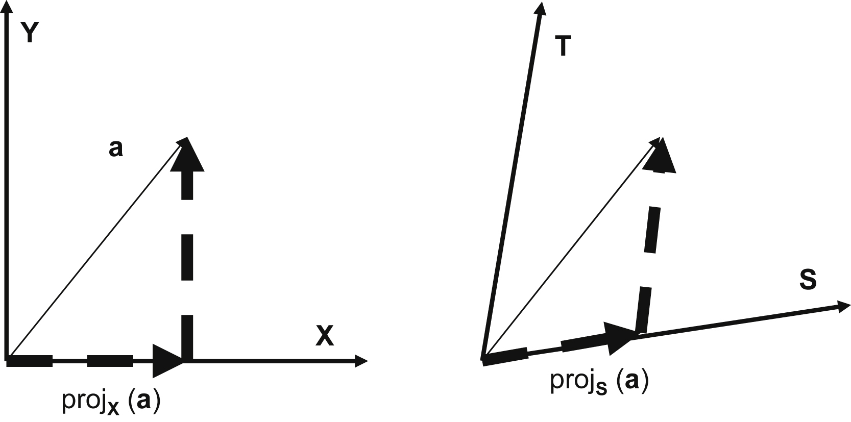
We now need to introduce the concept of projection. The projection of a vector is with respect to a reference vector. The projection is the component of a vector that is colinear or in the same direction as the reference vector. The remaining portion of the vector will be orthogonal to the reference vector. The projection is a scalar value, since the direction of the projection is by definition the reference vector direction (Fig. 13.9).

Dot<v₁, v₂> is the dot product of v₁, v₂ as defined in Fig. 13.2. The dot product produces a scalar result.

${Scaler proj}_{u} (a) = dot < u, a > / dot < u, u >$ ${Scaler proj}_{u} (a) = dot < u, a > / dot < u, u >$

Reference vectors do not need to be orthogonal, just independent. Any vector in n-space can be expressed as a combination of the n reference vectors. The q_i vectors are both independent and orthogonal. All of the a_i vectors can be expressed as linear combinations of q_i vectors, as defined by the values in the R matrix. By defining q₁ to be colinear or in same direction as a₁, this means a₁ is defined only by the scale factor of r_1,1. There is a two-dimensional plane defined by the vectors a₁ and a₂. The vector q₂ lies in this plane and is orthogonal to q₁. Therefore, a₂ can be defined as a linear combination of q₁ and q₂, defined by the scale factors of r_1,2 and r_2,2.

Using this, the q_i vectors and the values of the R matrix can be computed.

$\begin{matrix} q_{1} = u_{1} / norm (u_{1}) and u_{1} = a_{1} \\ q_{2} = u_{2} / norm (u_{2}) and u_{2} = a_{2} - {proj}_{u1} (a_{2}) \\ q_{3} = u_{3} / norm (u_{3}) and u_{3} = a_{3} - {proj}_{u1} (a_{3}) - {proj}_{u2} (a_{3}) \\ q_{4} = u_{4} / norm (u_{4}) and u_{4} = a_{4} - {proj}_{u1} (a_{4}) - {proj}_{u2} (a_{4}) - {proj}_{u3} (a_{4}) \\ q_{n} = u_{n} / norm (u_{n}) and u_{n} = a_{n} - {proj}_{u1} (a_{n}) - {proj}_{u2} (a_{n}) - {proj}_{u3} (a_{n}) \dots - {proj}_{u (n−1)} (a_{n}) \end{matrix}$ $\begin{matrix} q_{1} = u_{1} / norm (u_{1}) and u_{1} = a_{1} \\ q_{2} = u_{2} / norm (u_{2}) and u_{2} = a_{2} - {proj}_{u1} (a_{2}) \\ q_{3} = u_{3} / norm (u_{3}) and u_{3} = a_{3} - {proj}_{u1} (a_{3}) - {proj}_{u2} (a_{3}) \\ q_{4} = u_{4} / norm (u_{4}) and u_{4} = a_{4} - {proj}_{u1} (a_{4}) - {proj}_{u2} (a_{4}) - {proj}_{u3} (a_{4}) \\ q_{n} = u_{n} / norm (u_{n}) and u_{n} = a_{n} - {proj}_{u1} (a_{n}) - {proj}_{u2} (a_{n}) - {proj}_{u3} (a_{n}) \dots - {proj}_{u (n−1)} (a_{n}) \end{matrix}$

Q = {q₁, q₂, q_3… q_n} which is a matrix composed of orthonormal column vectors.

The upper triangular R matrix is the scalar coefficients of the projection.

$R = \begin{matrix} Dot < q_{1}, a_{1} > & Dot < q_{1}, a_{2} > & Dot < q_{1}, a_{3} > & \dots & Dot < q_{1}, a_{n} > \\ 0 & Dot < q_{2}, a_{2} > & Dot < q_{2}, a_{3} > & \dots & Dot < q_{2}, a_{n} > \\ 0 & 0 & Dot < q_{3}, a_{3} > & \dots & Dot < q_{3}, a_{n} > \\ 0 & 0 & 0 & \dots & Dot < q_{4}, a_{n} > \\ . & . & . & . & . \\ 0 & 0 & 0 & 0 & Dot < q_{n}, a_{n} > \end{matrix}$ $R = \begin{matrix} Dot < q_{1}, a_{1} > & Dot < q_{1}, a_{2} > & Dot < q_{1}, a_{3} > & \dots & Dot < q_{1}, a_{n} > \\ 0 & Dot < q_{2}, a_{2} > & Dot < q_{2}, a_{3} > & \dots & Dot < q_{2}, a_{n} > \\ 0 & 0 & Dot < q_{3}, a_{3} > & \dots & Dot < q_{3}, a_{n} > \\ 0 & 0 & 0 & \dots & Dot < q_{4}, a_{n} > \\ . & . & . & . & . \\ 0 & 0 & 0 & 0 & Dot < q_{n}, a_{n} > \end{matrix}$

Now, A = Q · R.

This can be verified by performing the matrix multiplication. For example, multiplying the first row of Q by the first column of R gives

$a_{1,1} = q_{1,1} \cdot r_{1,1} (since the other values of the r_{1} column are 0) = (a_{1,1} / norm (a_{1})) \cdot Dot < q_{1}, a_{1} > = a_{1, 1}$ $a_{1,1} = q_{1,1} \cdot r_{1,1} (since the other values of the r_{1} column are 0) = (a_{1,1} / norm (a_{1})) \cdot Dot < q_{1}, a_{1} > = a_{1, 1}$

13.6. QR Decomposition Restructuring for Parallel Implementation

The QR decomposition can also be expressed in code below. This would be typical for a serial implementation on a CPU. However, this would be inefficient for a parallel implementation, such as in a GPU or FPGA or other parallel processing device.

for k = 1:n
    r(k,k) = norm(A(1:m, k));
    for j = k+1:n
        r(k, j) = dot(A(1:m, k), A(1:m, j)) / r(k,k);
    end

    q(1:m, k) = A(1:m, k) / r(k,k);
    for j = k+1:n
         A(1:m, j) = A(1:m, j) - r(k, j) ∗ q(1:m, k);
    end
end

The algorithm can be restructured to allow taking advantage of the parallel implementation in a GPU or FPGA. The norm function can be replaced by a dot product and square root operation, which is often more efficient. Second, the first inner loop requires r(k,k) to be computed first, which has a longer latency. Third, the second inner loop requires q(1:m, k) to be computed first, which also has a long latency. To remove the data dependencies, the order of operations will be changed. All of the r terms will be calculated first. This can be before q_i is known.

for k = 1:n
    r(k,k) = norm(A(1:m, k));

r2(k,k) = dot(A(1:m, k), A(1:m, k);

r(k,k) = sqrt(r2(k,k));

    for j = k+1:n
        r(k, j) = dot(A(1:m, k), A(1:m, j)) / r(k,k);
        rn(k, j) = dot(A(1:m, k), A(1:m, j))
        r(k, j) = rn(k,j)/ r(k,k);
    end
    q(1:m, k) = A(1:m, k) / r(k,k);
    for j=k+1:n
         A(1:m, j) = A(1:m, j) - r(k,j) ∗ q(1:m,k);
    end
end

Next, the following substitutions can be performed in the second inner loop. Replace r(k,j) with rn(k,j)/r(k,k) and replace q(1:m,k) with A(1:m,k)/r(k,k).

for k = 1:n
    r2(k,k) = dot(A(1:m, k), A(1:m,k);
    r(k,k) = sqrt(r2(k,k));
    for j = k+1:n
        rn(k, j) = dot(A(1:m, k), A(1:m, j));
        r(k, j) = rn(k,j)/ r(k,k);
    end
    q(1:m, k) = A(1:m, k) / r(k,k);
    for j = k+1:n
         A(1:m, j) = A(1:m, j) - r(k,j) ∗ q(1:m,k);
         A(1:m, j) = A(1:m, j) - rn(k,j)/ r(k,k) ∗ A(1:m,k) / r(k,k);
    end
end

Then operations can be reordered into two functional groups. Every r term depends on the norm of the first column for the current iteration, the calculation of which requires a deep pipeline. The same datapath used for the vector product required for the norm can also be used to calculate the vector operation for each r term. All vector operations for the r term calculation, <v_i,v_i> for r_ii, and <v_j,v_i> for r_ij can be issued on subsequent clock cycles.

Following the vector operations, a separate function can be used for the square roots and inverse square roots. The square root and divide operations are scheduled as late as possible, after the vector operations. All of the r terms can therefore be calculated without any data dependencies, once the pipeline is full.

(first computational group)

for k = 1:n
    r2(k,k) = dot(A(1:m, k), A(1:m,k);
    for j = k+1:n
        rn(k, j) = dot(A(1:m, k), A(1:m, j));
    end
    for j = k+1:n
         A(1:m, j) = A(1:m, j) − (rn(k,j) / r2(k,k)) ∗ A(1:m,k);
    end
end

(second computational group)

for k = 1:n
    r(k,k) = sqrt(r2(k,k));
    for j = k+1:n
        r(k, j) = rn(k,j)/ r(k,k);
    end
    q(1:m, k) = A(1:m, k) / r(k,k);
end

The upper loop can run with few stalls, as there are no long latency math operations. This is where the bulk of the computation is performed. The r terms are then used as one of the inputs to the vector multiplier, the first column for the outer loop is generated, and all of the subsequent columns updated. The only data dependency is between the first r term output of the datapath and the start of the q_i vector calculation, which may introduce a wait state between the two parts of the inner loop. As the pipeline depth of the datapath will be fixed, but the inner loop reduces by one with each pass, wait states may be required at some point in the processing of the matrix, which once started, will gradually increase by each pass.

The lower loop can run as data become available and are relatively latency insensitive. In this way, the computational units can avoid unnecessary stalls, which can improve the matrix processing throughput.

..................Content has been hidden....................

You can't read the all page of ebook, please click here login for view all page.

Table of Contents for Chapter 13. Matrix Inversion

Create new playlist

Sign In

Sign Up