In previous chapters, the use of Doppler processing was discussed as a key method to discriminate both in distance and velocity. Discrimination in direction (or angle of arrival to the antennas) is provided by aiming the radar signal, using either traditional parabolic or more advanced electronic steering of array antennas.
Under certain conditions, other methods are required. For example, jammers are sometimes used to prevent detection by radar. Jammers often emit a powerful signal over the entire frequency range of the radar. In other cases, a moving target has such a slow motion that Doppler processing is unable to detect against stationary background clutter—such as a person or vehicle moving at walking speed. A technique called space time adaptive processing (STAP) can be used to find targets that could otherwise not be detected.
Keywords
AESA; Interference covariance matrix; Radar data cube; Space time adaptive processing; Steering vector
In previous chapters, the use of Doppler processing was discussed as a key method to discriminate both in distance and velocity. Discrimination in direction (or angle of arrival to the antennas) is provided by aiming the radar signal, using either traditional parabolic or more advanced electronic steering of array antennas.
Under certain conditions, other methods are required. For example, jammers are sometimes used to prevent detection by radar. Jammers often emit a powerful signal over the entire frequency range of the radar. In other cases, a moving target has such a slow motion that Doppler processing is unable to detect against stationary background clutter—such as a person or vehicle moving at walking speed. A technique called space time adaptive processing (STAP) can be used to find targets that could otherwise not be detected.
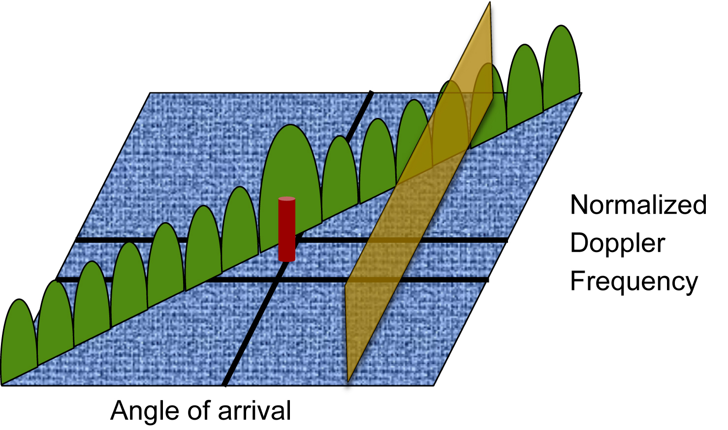
Because the jammer is transmitted continuously, its energy is present in all the range bins. And as shown in Fig. 21.1, the jammer cuts across all Doppler frequency bins, due to its wideband, noiselike nature. It does appear at a distinct angle of arrival, however. Fig. 21.1 also depicts the ground degree of clutter in a side-looking airborne radar, due to the Doppler of the ground relative to the aircraft motion. A slow-moving target return can easily blend into the background clutter.
Figure 21.1 Clutter and jammer effects in Doppler space.
STAP radar could provide benefits in automotive applications. Metallic vehicles provide strong reflections of the radar pulses. Doppler processing allows for the radar to easily distinguish the radar returns from moving vehicles compared to the background clutter. One issue with traditional radar systems is that desensitization by interfering signals, perhaps even from another automotive radar system. Detecting nonmetallic and slow moving subjects such as pedestrians, bicyclists, and animals against stationary background clutter is difficult for traditional radar systems, and normally camera-based systems are used for this purpose. However, a camera-based system can be impaired by low-light conditions, weather, or any other circumstances that cause poor visibility. A possible solution to all of these issues is to integrate STAP into the radar system.
Linear algebra and matrix operations are used in STAP. For those unfamiliar with this, please refer Chapter 13 on matrix operations and inversion.
21.1. Space Time Adaptive Processing Radar Concept
STAP radar processing is combining temporal and spatial filtering that can be used to both null jammers and detect slow-moving targets. It requires very high numerical processing rates, as well as low latency processing, with dynamic range requirements that generally require floating-point numerical representation.
STAP processing requires use of an array antenna. However, in contrast to the active electronically scanned array (AESA), for STAP the antenna receive pattern is not electronically steered as with traditional beamforming arrays. In this case, the array antenna provides the raw data to the STAP radar processor, whereas the antenna processor does not perform the beam steering, phase rotation, or combining steps, as indicated in Fig. 21.2. The directional processing is done in a later stage as part of the STAP algorithm. Also, while the AESA is depicted in one dimension, this array can and often is two dimensional, in both elevation (up and down) and azimuth (side to side). In this way, the antenna receive pattern can be steered or aimed in both elevation and azimuth.
Figure 21.2 Antenna array allowing directional processing. STAP; space time adaptive processing.
The radar processing can occur over N consecutive pulses, as long as they lie within the coherent processing interval, considered “slow” time. In the case of the automotive radar system considered here, N=256. Performing STAP processing over all 256 pulses simultaneously would result in hundreds of TFLOPs of processing power. A common technique is to break the radar data cube into smaller sections, perform STAP on them individually, and then integrate the detection results from the separate computations.
In this case, 16 pulses will be used for STAP to bring the processing requirement to a reasonable level, and this will divide the radar data cube into 16 sections (as there are 256 pulses in the radar frame). To ensure the maximum Doppler sensitivity, the selected pulses will not be contiguous but rather will be data from every 16th pulse. Then the first STAP dataset would be over pulses {0, 16, 32, 48, 64, 80, 96, 112, 128, 144, 160, 176, 192, 208, 224, 240}. Then a second STAP dataset would be performed over pulses {1, 17, 33, 49, 65, 81, 97, 113, 129, 145, 161, 177, 193, 209, 225, 241}. Using datasets containing pulses spread over a longer interval (14ms) means there will be more relative moment resulting in greater Doppler shift, which should provide better detection.
With airborne radar trying to detect slow-moving targets on ground, the range to the suspected targets of interest to perform STAP is known. This is not the case for automotive radar. Therefore, it will be suggested that the processing be performed at ranges of 20, 40, 60, and 80m, which should allow timing detection of pedestrians, animals, or cyclist. However, detailed simulations and field testing will be required to fully optimize these radar processing configurations.
The L=512 radar samples collected during the pulse interval are binned, and after fast Fourier transform (FFT) processing, corresponds to the range. The range sampling rate is referred to as “fast” time in radar jargon, whereas processing across the pulses is referred as “slow” time.
STAP radar will operate on the postrange-FFT processed cube of data, shown in Fig. 21.3. The M dimension corresponds to the number of inputs from the array antenna. The resulting radar data cube will be of dimensions M (number of array antenna inputs) by L (number of range bins in fast time) by N (number of pulses in slow time). Doppler processing, which is not part of STAP, occurs over the data slice across the L and N dimensions. In STAP, arrays of data (or slices) across the M and N dimensions are processed.
STAP is basically an adaptive filter that can filter over the spatial and temporal (or time) domain. The goal of STAP is to take a hypothesis that there is a target at a given location and velocity and create a filter that has high gain for that specific location and velocity and proportional attenuation of all signals (clutters, interferers, and any other unwanted returns). There can be many returns of interest to generate location and velocity hypothesis for, and these are all normally processed together in real time. This produces very high processing and throughput requirements on the STAP radar processor.
Figure 21.3 Radar data cube used in Space Time Adaptive Processing radar.
This brings up the issue of how the spatian and Doppler hypotheses for the weak returns are identified for subsequent STAP processing. This can come from weak detections found in normal pulse-Doppler processing or information from other sensor systems; in an auto radar, from ADAS camera-based sensors or IR sensors on the vehicle.
STAP has the capability to pull targets that are below the clutter into a range that can be reliably detected. A good analogy is a magnifying glass. Conventional methods are used to view the big picture, but if something of interest is noted, STAP can be used to act as a magnifying glass to zoom into a specific area and see things that would be otherwise undetectable.
21.2. Steering Vector
For each suspected target, a target steering vector must be computed. This target steering vector is formed by the cross product of the vector representing the Doppler frequency and the vector representing the antenna angle of elevation and azimuth. For simplicity, we will assume only azimuth angles are used.
The Doppler frequency offset vector is a complex phase rotation:
Fd=e−2π⋅n⋅Fdoppforn=1…N−1
The spatial angle vector is also a phase rotation vector:
The target steering vector t is the cross product vector Fd and Aθ as shown in Fig. 21.4, and t is vector of length N·M. This must be computed for every target of interest. Assuming 12 antennas, and that every 16th of the 256 pulse data is used, the vector t is 16×12=192 complex samples long.
21.3. Interference Covariance Matrix
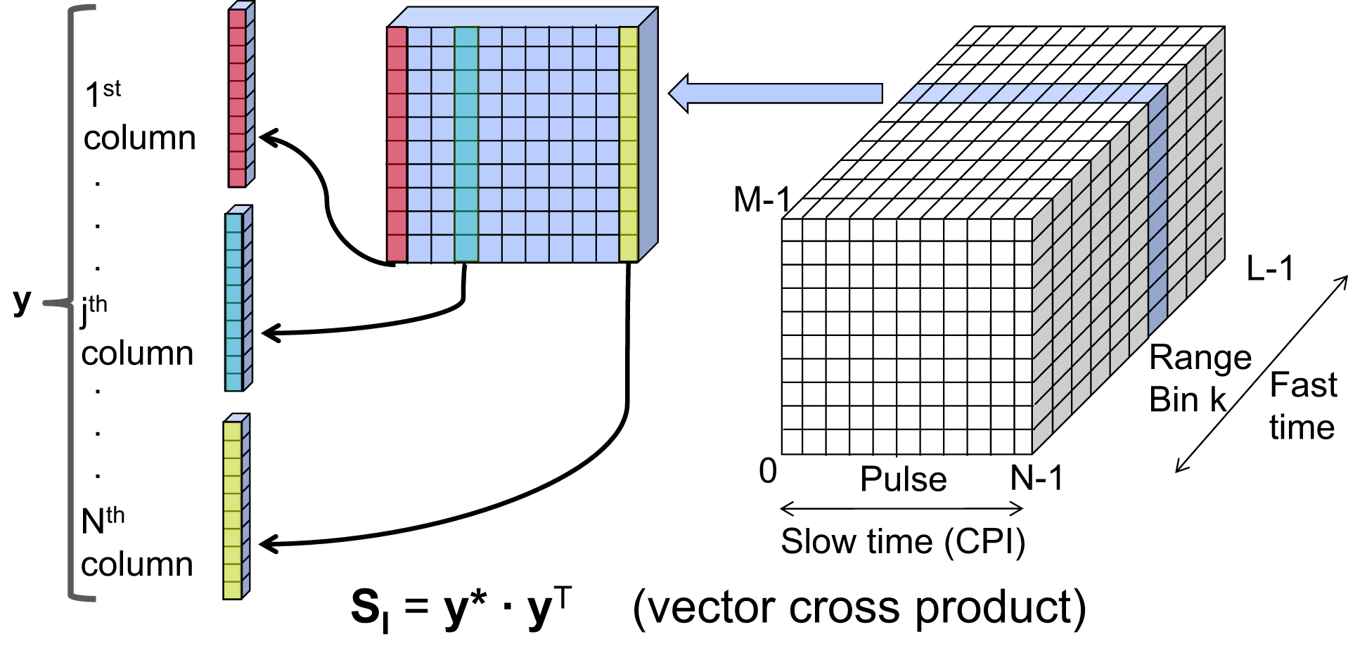
The interference covariance matrix SI must be estimated. A common method is to just compute and average this for many range bins surrounding the range of interest. To compute this, a column vector y is built from a slice of the radar data cube at a given range bin k. The covariance matrix by definition will be the vector cross product:
SI=y∗⋅yT
Here the vector y is conjugated and then multiplied by its transpose. As y is of length N·M, the covariance matrix SI is of size [(N·M)×(N·M)] as shown in Fig. 21.5. This is a matrix of [192,192] for the configuration being considered. All the data and computations are being done with complex numbers, representing both magnitude and phase. An important characteristic of SI is that it is Hermitian, which means that SI=SI∗T or equal to its conjugate transpose. This symmetry is an inherent property of covariance matrices.
The covariance matrix represents the degree of correlation across both antenna array inputs and over the group of pulses. The process is to characterize undesired signals, and create an optimal filter to remove them, thereby facilitating detection of the target. The undesired signals can include noise, clutter, and interfering signals.
SInterference=Snoise+Sinterferingsignal+Sclutter
The covariance matrix is very difficult to calculate or model; therefore, it is estimated. Since the covariance matrix will be used to compute the optimal filter, it should not contain the target data. Therefore, it is not computed using the range data right where the target is expected to be located. Rather, it uses an average of the covariance matrices at many range bins surrounding but not at the target location range as shown in Fig. 21.6. This average is an element by element average for each entry in the covariance matrix, across these ranges. This also means that many covariance matrices need to be computed from the radar data cube. The assumption is that the clutter and other unwanted signals are highly correlated to that at the target range, if the difference in range is reasonably small.
The estimated covariance matrix can used to build the optimal filter that involves inversion of the covariance matrix, which is computationally very expensive, and generally requires the dynamic range of floating-point numerical representation. The matrix is of size [(N·M)×(N·M)] and can be quite large.
Figure 21.6 Estimating covariance matrix using neighboring range bin data.
21.4. Space Time Adaptive Processing Optimal Filter
Fortunately, the matrix inversion result can be used with multiple targets at the same range. The steps are as follows:
SI⋅u=t∗,oru=SI−1⋅t∗
One method for solving for SI is known as QR decomposition, which will be used here. Another popular method is the Cholesky decomposition, as the interference covariance matrix is Hermitian symmetric.
Perform the substitution SI=Q·R, or product of two matrices.
Q and R can be computed from SI using one of several methods, such as Gram–Schmidt, Householder transformation, or Givens rotation. The nature of the decomposition into two matrices is that R will turn out to be an upper triangular matrix, and Q will be an orthonormal matrix, or a matrix composed of orthogonal vectors of unity length. Orthnonormal matrices have the key property as follows:
Q⋅QH=IorQ−1=QH
Therefore it is trivial to invert Q. Please refer to the chapter on matrix inversion (Chapter 13) for more detail on QR decomposition.
Q⋅R⋅u=t∗thenmultiplybothsidesbyQH
R⋅u=QH⋅t∗
Since R is an upper triangular matrix, u can be solved by a process known as “back substitution.” This started with the bottom row that has one nonzero element and solving for the bottom element in u. This result can be back-substituted for the second to bottom row with two nonzero elements in the R matrix, and the second to bottom element of u solved for. This continues until the vector u is completely solved. Notice that since the steering vector t is unique for each target, the back-substitution computation must be done for each steering vector.
Then solve for the actual weighting vector h.
h=u/(tH·u∗), where dot product (tH·u∗) is a weighting factor (this is a complex scaler, not vector).
Finally solve for the final detection result z by the dot product of h and the vector y from the range bin of interest.
z=hT⋅y
z is a complex scaler, which is then fed into the detection threshold process. Over the 16 STAP processes, the values can be integrated for each of the range and steering vector locations.
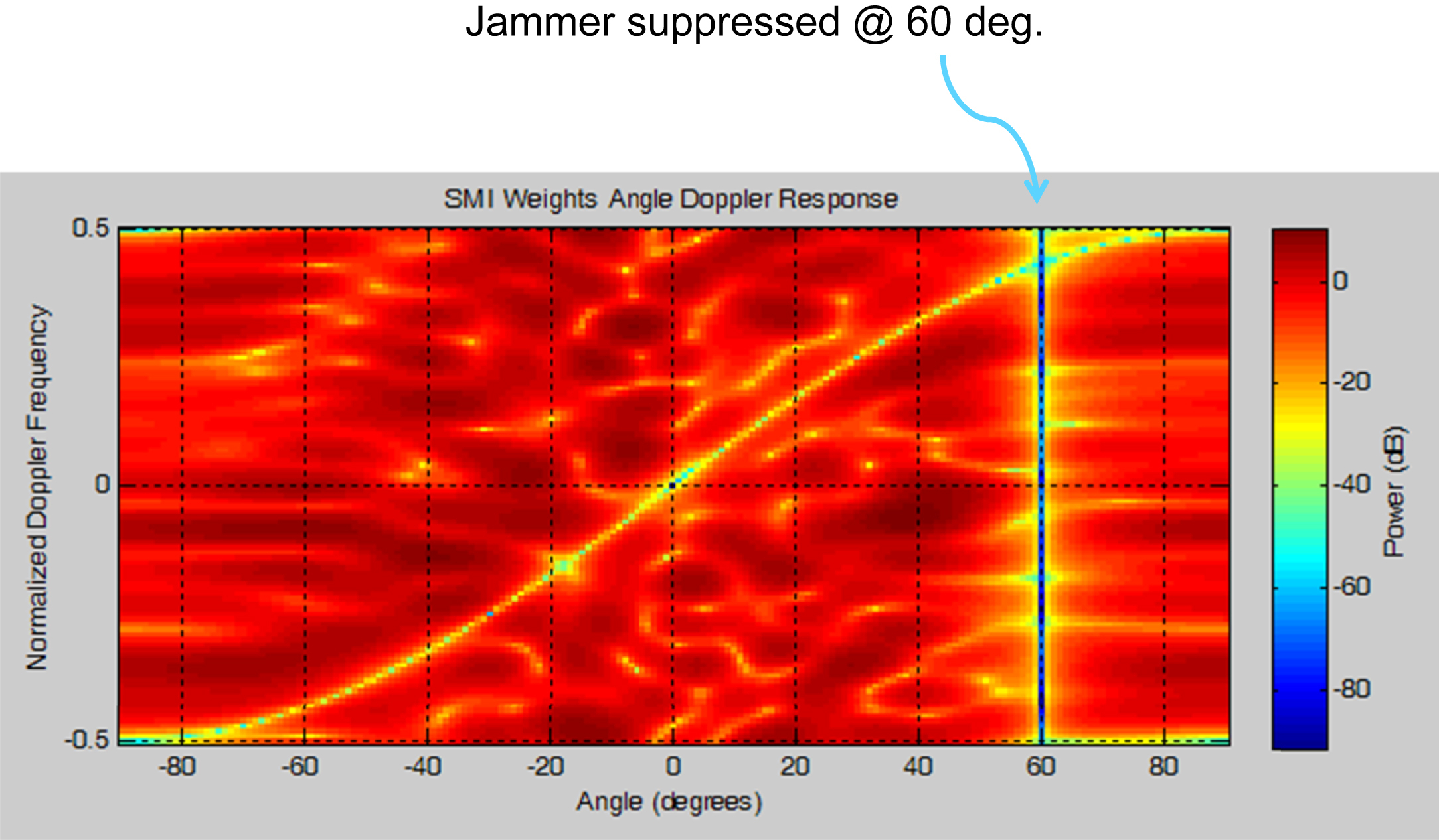
Shown in Fig. 21.7 is a plot of SI−1, the inverted covariance matrix. In this case, there is an interfering signal at 60 degrees azimuth angle, and a target of interest at 45 degrees, with range of 1723m normalized Doppler of 0.11. Note that this is for an airborne radar scanning the ground searching for slow-moving targets, hence the longer range.
Notice the very small values, in the order of −80dB, present at 60 degrees. The STAP filtering process is detecting the correlation associated with the interfering signal direction at 60degrees. But inverting the covariance matrix, this jammer will be severely attenuated. Notice also the diagonal clutter line. This is a side-looking airborne radar, so the ground clutter has positive Doppler looking in the forward direction or angle and negative Doppler in the backward direction or angle. This ground clutter is being attenuated at about −30dB, proportionally less severely than the more powerful interfering signal.
The target is not present in this plot. Recall that the estimated covariance matrix is determined in range bins surrounding but not at the expected range of the target. But in any case, it would not likely be visible anyway. However, the use of STAP with the appropriate target steering vector can make a dramatic difference, as shown in Fig. 8. The top plot shows the high return of the peak ground clutter at range of 1000m with magnitude of ∼0.01, and noise floor of about ∼0.0005.
Figure 21.7 Logarithmic plot of inverted covariance matrix.
Figure 21.8 Space time adaptive processing (STAP) gain.
With STAP processing, the noise floor is pushed down to ∼0.1×10⁻⁶ and the target signal at about 1.5×10⁻⁶ is now easily detected. It is also clear that floating-point numerical representation and processing will be needed for adequate performance of the STAP algorithm.
The STAP method described is known as the power domain method. It is the called power domain because the covariance matrix estimation results in squaring of the radar data, hence, the algorithm is operating on signal power. This also increases the dynamic range of the algorithm, but this is easily managed as floating point is being used for all processing steps.
21.5. Space Time Adaptive Processing Radar Computational Requirements
It is necessary to consider the processing requirements as shown in Table 21.1. Using the following assumptions:
Pulse repetition frequency (PRF)=1000Hz
12 antenna array inputs (Aθ vectors are of length 12 or M=12)
16 pulse processing (Doppler vectors are of length 16 or N=16)
Minimum required size of SI is 192×192, in complex single precision format
Assume 32 likely targets to process (32 target steering vectors)
Use of 200 range bins to estimate SI
This actually is a very conservative scenario. The PRF is rather low, and the number of antenna array inputs is very small. Should the number of antenna array inputs increase by 12–48, the processing load of the matrix processing, in particular QR decomposition goes up by the third power or 64 times. This would require over 3 TFLOPS of floating-point processing power. Because of this the limitations on STAP are clearly the processing capabilities of the radar system.
Table 21.1
Space Time Adaptive Processing GFLOPs Estimate
STAP Processing Steps
Approximate Computational Load
Compute covariance matrices
23 GFLOPs
Average over 200 matrices to find estimated SI
8.0 GFLOPs
QR decomposition
37.7 GFLOPs
Compute QH·t∗ for 32 targets
9.4 GFLOPs
Solve for u using back substitution
4.7 GFLOPs
Compute h=u/(tH·u∗) and z=hT·y
0.2 GFLOPs
Total
83 GFLOPs
The theory of STAP has been known for a long time, but the processing requirements have made it impractical until fairly recently. Many radar applications benefiting from STAP are airborne and often have stringent size, weight, and power (SWaP) constraints. Very few processing architectures can meet the throughput requirements of STAP, and even fewer can simultaneously meet the SWaP constraints. As most radars operate in a continuous manner, receiving an enormous amount of data, this data normally must be processed in real time using powerful compute devices or accelerators. These are commonly graphics processing units or field programmable gate arrays in many radar systems.