Chapter 14
Field-Oriented Motor Control
Abstract
Electric motors have been ubiquitous for 100 years or more and were controlled using mechanical or analog methods. Today, motors are increasingly digitally controlled, which can provide greater performance, reliability, and efficiency. This chapter will first give an overview of electric motor theory and operation and then introduce a basic digital motor control algorithm known as field-orientated control.
Keywords
AC motor; Back EMF; Clark transform; DC motor; Field-oriented control; Induction motor; Magnetic flux; Park transform; PID controller
Electric motors have been ubiquitous for 100 years or more and were controlled using mechanical or analog methods. Today, motors are increasingly digitally controlled, which can provide greater performance, reliability, and efficiency. This chapter will first give an overview of electric motor theory and operation and then introduce a basic digital motor control algorithm known as field-orientated control, or FOC.
14.1. Magnetism Basics
In the 1800s Michael Faraday speculated that magnetic fields exist as lines of force, which we today refer to as “magnetic flux,” which is measured in units of “Webers.” Essentially, the more flux there is, the stronger the magnet will be. We conventionally think of flux leaving the north pole and reentering the south pole of a magnet, as shown by the arrows in Fig. 14.1. If we measure how much flux cuts through a surface area which is perpendicular to the flux path, it provides a measure of the flux density at that particular spot in space. One Weber of flux cutting through one square meter of area constitutes a flux density of one “Tesla,” named after Nikola Tesla, who is also the inventor of the AC induction motor (ACIM).

Also in the early 1800s, Hans Christian Oersted discovered that current flowing in a wire creates its own magnetic field, and when this field interacts with a second magnetic field, the result is a force acting on the conductor. This force is proportional to the amount of current flowing in the wire, the strength of the second magnetic field, and the length of wire that is affected by the second magnetic field. The direction of the force can be determined by a technique know as the right-hand rule. If your right hand is configured as shown below, where your thumb points in the direction of positive current flow and your index finger points in the direction of the second magnetic field's flux (i.e., flowing from the north pole to the south pole), then your middle finger will be pointing in the direction of the force acting on the wire, as shown in Fig. 14.2.
The back EMF (electromotive force) is the voltage generated in a loop of wire caused when the magnetic flux enclosed by that loop is changing. This can result in several ways. The intensity of the magnetic flux level may be controlled by an adjustable source. Or it could be caused if the flux field is moving relative to the loop of wire, or if the loop of wire itself is rotating in the magnetic flux field or both. This effect led to “Faraday's Law,” which states that the voltage generated in a loop of wire is equal to the rate at which the magnetic flux threading through that loop of wire is changing.
Using the right-hand rule, this can be applied to a rotating system. In this case, we can see the cross section of a cylinder, which is once again rotating in a uniform magnetic field. A wire is placed about the cylindrical cross section, as shown in Fig. 14.3.
From Faraday's law, the voltage that will be generated through this wire (from one end to the other) is equal to the rate of change of the flux threading through the loop. Even though the flux of the magnetic field is of constant strength, the cross-sectional area of the loop with respect to the magnetic field changes by rotating the wire loop. When the loop of wire is straight up and down (vertically orientated), the loop area collapses to zero, and this is the fastest rate of flux change, and therefore when the peak voltage is generated. When the loop of wire is orientated perpendicular to the flux field, the rate of change of the loop area is zero at that instantaneous moment, producing no voltage. Therefore, as the loop rotated, the voltage induced will be sinusoidal, centered about zero.


This effect can be multiplied, by replacing a single loop of wire with N loops of wire, all connected together in series. The voltages from each loop add together in series, creating a much higher voltage, which has the same effect as multiplying the flux in the loop by a factor of “N.” The total rate of change of the flux changes as a function of the rotational angle, the number of turns, the field strength, and the geometry of the machine and generates an AC waveform as the machine rotates.
14.2. AC Motor Basics
Using the same principals, a motor can be driven from an AC voltage (Fig. 14.4). The rotor (rotating part) is composed of a permanent magnet, and the AC voltage is used to magnetize the stator (stationary portion). The stator acts as an electromagnet, excited by the AC waveform. The magnetic field is implemented by coil of wire, and effect of this can be magnified by using soft iron core, which becomes magnetized and conducts the magnetic flux. The rotor will rotate at the same frequency as the AC voltage frequency, as the permanent magnet will follow the magnetic polarity of the stator.
A multiphase AC motor can also be constructed. Three phases are common in high-power industrial motors, with each phase 120 degrees relative to the others. The coils of each phase are interleaved around the stator.

14.3. DC Motor Basics
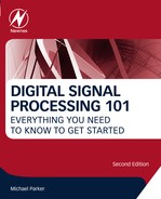
A motor can also be driven by a DC voltage. In this a form of commutation must be implemented, to create a rotating magnetic field. In this case, permanent magnets are used in the stator, not in the rotor (Fig. 14.5). The rotor is an electromagnet, which can have multiple coils of wire wound about the iron cores mounted on the rotor shaft. The electromagnets in the rotor are excited when contact is made through the brushes, using DC current. When the shaft has rotated 180 degrees the same DC current will flow in the opposite direction through the wire coil, exciting the same electromagnet in the opposite polarity. Several coils and brush contacts can be interleaved about the shaft, each making contact as the shaft rotates and exciting each rotor coil in turn.

The disadvantage of DC brush motors is that the mechanical commutation provided by the brushes requires periodic brush replacement due to erosion, and the large amount of electromagnetic induction (EMI) generated by the rotor's sparking as they make and break contact. A further disadvantage is torque ripple, which can result in vibration. This is due to changes in torque as the angular relationship changes due to rotation. The peak torque occurs when the rotor electromagnet is orthogonal to the stator magnets and zero torque when the rotor electromagnet is aligned with the stator magnet. At this moment, the brushes will break contact, and then reconnect with current flowing in the opposite direction. In this way, a net torque is maintained in one rotational direction. However, the torque will be sinusoidal in nature, resulting in torque ripple and mechanical vibration (Fig. 14.6).
14.4. Electronic Commutation
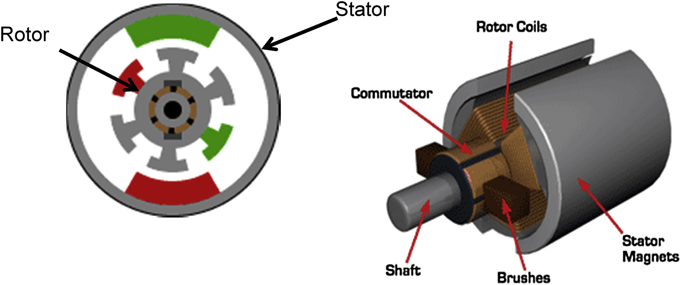
Alternately, the DC motor can be electrically commutated. The basic structure used is the “H” bridge (Fig. 14.7), which depending on which transistors are switched on, can drive DC current in either direction through a wire coil. There is no need for brushes, which are a maintenance concern. And the current waveform can be changed as rapidly as necessary, without any mechanical limitation.
A BLDC (brushless DC) motor is like a brush DC motor turned inside out. To make the motor spin, the current is switched from one set of coils to the next. Normally, three is the minimum number of phases used (Fig. 14.8). Motor speed can be controlled by the rate of the electrical communication, providing for means of regulating the motor's rotational speed. However, this assumes the motor is able to rotate at the rate of the commutation with a given load. Generally, an electrically commutated motor must have some means of feedback providing the rotational position of the rotor at any given instant.


A more efficient commutation is to turn on more than one set of coils at a time, to provide more torque in the motor. Here there are two coils energized at the same time so that when one coil has positive current, the other energized coil has negative current. A clever way to use the same current in both coils is to connect all the coils together inside the motor, called a “Y”-connected winding pattern. The current waveforms for each winding are shown in Fig. 14.9. The commutation sequence provides a complete 360 degrees rotation of the motor, with each phase being 120 degrees relative to the others. Because in each state there are two coils energized, and one coil idle, this provides for greater motor torque that a motor commutated with only one coil active at a given time.
Another benefit over brush commutation is that the current can be switched on and off very rapidly, much of that can be used to create more complex current waveforms. Normally, a linear amplifier or a variable voltage source would be necessary to create a current waveform with different levels. However, this same effect can be created by switching the current very rapidly from a constant or DC power source. This is known as pulse width modulation (PWM). The duty cycle, which is the ratio of “ON” time to the total period of the switching frequency, determines the average amount of current flow. This requires a transistor switching frequency to be much higher than the motor commutation rates. This waveform is then filtered by the inductance in the motor to smooth or average the current output waveform. A sinusoidal waveform is often used and provides the most efficient and smoothest (minimum torque ripples) operation (Fig. 14.10).
Creating a sinusoidal waveform from a DC source to commutate a motor is starting to look a lot like an AC motor, since the stator coils must be driven by some type AC waveforms to cause motor rotation. Therefore, motors of this type are often called BPM or brushless permanent magnet motors. The motor is electrically commutated and has permanent magnets in the rotor. Two types of BPM motors are the BLDC motor, which is driven by “square” wave current modulation, and PMAC (permanent magnet AC) motor, which is driven by sinusoidal current modulation. There are further distinctions with regard to the types of permanent magnets used in rotor.

All of the brushless motors described do require a means of determining the rotational position and speed of the rotor to be able to properly energize the coils in an optimal manner to control the motor behavior (Fig. 14.11). Some applications require precise rotational position. For this method, it is common to mount hall-effect types of sensor on the rotor shaft. Using two hall-effect sensors with a 90 degrees shift in their pattern provides the means to determine the direction and amount of rotation and is known as a quadrature encoder. Other applications require precise control of the motor torque. This is commonly done by sensing the motor drive currents, which are proportional to the torque generated by the motor. Other more advanced methods have been developed, which are sensorless. These methods monitor the back EMF of the motor stator windings and use that to estimate the motor speed. A drawback of this method is that back EMF is difficult to measure at low motor speeds.

14.5. AC Induction Motor
The last type of motor that will be covered is one of the most popular. It is the ACIM and is the most common type of motor used in both household and industrial applications. This motor is extremely simple and elegant, as well as can be very efficient, especially under constant load applications. It has no brushes and no magnets. It can be driven by AC waveforms provided directly from the electrical utility (no commutation mechanism required) or by AC waveforms generated using electronic commutation. The use of sensors is optional in the ACIM, particularly when the motor is driven directly from AC utility grid current. The ability to dispense with magnets, commutation circuits or brushes, and sensors makes the ACIM extremely reliable and economical for applications where precise rotational speed is not necessary—one common example is an industrial pump.
The key innovation is the rotor. The rotor contains multiple closed loops of wire. They are actually mounted at a slight angle to the rotor axis, as can be seen in Fig. 14.12. The stator is excited by AC waveforms. This will cause a changing magnetic flux through the closed coil within the rotor. Recall Fig. 14.3, depicting how a changing flux enclosed by a wire will cause EMF or voltage to be generated. If the wire is a close loop, this EMF voltage will cause a large flow of current in the wire loop. Current is induced in the rotor circuit from the stator circuit; much the same way that secondary current is induced from the primary coil in a transformer. This in turn will generate a magnetic field with its own flux, just as a permanent magnet in the rotor would. The torque generated will be proportional to the strength of the rotor magnetic field generated in the rotor coils, which will in turn be proportional to the rate of change of the flux through the rotor coils, which in turn is proportional to the rate at which the AC waveforms are changing. Now consider two cases. The first being when the rotor is stationary, which would be the condition on start-up of the motor. This provides the maximum rate of flux change between the rotating stator field and the stationary rotor coils. This will, therefore, be the maximum torque, which is a very desirable condition on start-up of the motor. The second case would be when the rotor is rotating at the same rate as the stator magnetic field. In this case, there is no change of flex through the rotor coils and, therefore, there is no current generated in rotor coils, and as a result no torque will be generated.

The normal operating condition of the ACIM motor is the “slip” condition. At steady state, the motor rotation speed will be such that the difference between the stator magnetic field rotational rate and the rotor rotational rate will produce a torque equal to the mechanical load. Should the load increase, the motor will slow further, having more “slip” that will result in more torque. If all the mechanical load is removed, the rotor will spin at almost the same rate as the stator magnetic field, with just enough slip to generate the torque required to overcome the bearing friction. If the AC stator currents are at a fixed frequency, such as on the grid generated by a centralized power plant, then the rotational speed will depend on the motor load, as just described.
For example, consider a three phase AC motor connected to the public grid with a frequency of 60 Hz. The motor will have stator windings A, B, and C for each of the three phases with each 120 degrees out of phase with the other. If, for example, the windings are replicated four times then the effective rotational speed of the stator commutation will be 60 Hz. Under no load, the rotor will spin at 60 revolutions per second, or 3600 RPM. If a load is placed on the motor to sufficiently cause a 5% slip, then the rotor will spin at 3420 RPM (Fig. 14.13).
The rotor has multiple windings of closed loops of wire, which are energized due the EMF due to the change in stator flux enclosed by the windings.
However, if the both the frequency and amplitude of the stator AC waveforms are generated from a DC source (using three “H” bridge circuits) and controlled, then the motor speed can also be controlled under dynamic load conditions, using an algorithm with closed loop feedback. One example might be an induction motor in an electric car powered by DC voltage batteries.

14.6. Motor Control
Every motor control loop follows the basic diagram in Fig. 14.14. The input to the controller is the desired behavior, which in the case of motors are usually speed and/or position. The controller also receives feedback from the motor indicating the actual motor speed/position. The desired input is subtracted from the actual input state, and this provides an error signal to the controller. The controller will then produce an output to the motor commutator that will minimize, or drive to zero the error signal.
A common controller type is the proportional integral derivator (PID) controller. It is so named because error signal is split into three separate paths of P, I, and D, which each produces a signal to motor circuit, which is summed together (Fig. 14.15). Each of these circuits has a separate gain constant. “P” stands for “proportional” and is the most intuitive. The larger the error signal, the larger will be the signal to the motor, to drive motor error to zero. “I” stands for “Integral,” and this term is designed to prevent a permanent, residual error. With just a P signal, as the motor approaches the desired position/speed, the correction will approach zero. This can result in a permanent difference. For example, if the motor controller is controlling only motor speed, a “P” control circuit will have the motor approach but never quite reach the desired speed. That is where the “I’’ circuit comes in. It will integrate the error over time, and if a permanent small lag in motor speed is present, this will build up in the “I” circuit, and drive this error signal to zero. Finally, the “D” stands for “differential.” The P and I terms function as described previously. The D path involves taking the derivative of the error signal. This can provide a more rapid response, as when the error signal suddenly begins to increase, it will provoke a vigorous response from the controller. This can cause instability, so often the D path is not used or set to zero. There are detailed mathematical methods to analyze control loops, and analyzing the stability and responsiveness of the control loop. An unstable control loop can oscillate. An underdamped control loop can overshoot, and an overdamped control loop can cause sluggish response. The setting of the P, I, and D gain coefficients is designed to provide proper controller response for a given system. Considerable simulation is normally used to determine the optimum values of P, I, and D.


Control loops can be designed to control a variety of aspects of a motor's operation. Here we are going to consider a common method, called FOC that is used to control the motor's torque, in particular for an AC motor, either induction or with a permanent magnet rotor. This control circuit can be used when the desired input signal corresponds to torque (such as the accelerator petal on an electric vehicle). Or it can be used in conjunction with other control loops, which may be controlling motor velocity or position. For example, if the input signal is a certain motor velocity, the output of the velocity controller will be a torque request signal, since an increase or reduction in torque is used to change motor velocity as needed to match the desired input velocity. Nested control loops are shown in Fig. 14.16.
The control loops can be implemented in hardware or a suitable real-time microprocessor. The PWM circuits, invertor, and analog-to-digital convertor are implemented in hardware. Provision for interfacing and processing motor feedback is also often included.
The current for a three phase electric motor can be generated in the inverter using three “H bridge” circuits, each producing a sinusoidal current that is 120 degrees relative to the others. This will result in a smoothly rotating magnetic flux pattern with frequency equal the frequency of the AC waveform. This can be thought of as a rotating vector, with the direction of the vector indicating the net phase associated with the stator flux at any given instant. A permanent magnet rotor will have a magnetic flux vector that rotates with the rotor mechanical motion. With an ACIM, the rotor will be magnetized by the changing flux of the stator, and the induced EMF will cause current flow and a magnetic flux in the rotor coils. Owing to the rotor slip in an ACIM, the flux is changing in the rotor coils, in response to the relative rotation of the stator flux vector. Note that while the rotor mechanical rotary speed will be less than the stator AC current vector rotation, the induced the magnetic flux vector rotation is synchronous with the stator AC current vector.
The difference between the stator and rotor magnetic flux vectors can be expressed in degrees of phase, similar to describing the phase difference in two sinusoidal waves (Fig. 14.17). At zero phase difference, there will be no torque generated. The forces generated by the interacting magnetic fields are in an axial direction to the motor shaft, which only results in force on the motor bearings, but does not produce any rotational force (designated as “d” direction). A phase difference or lag in the stator and rotor magnetic fluxes will produce a rotational force and generate torque. When the phase lag is 90 degrees, all of this force will be directed toward rotating the motor shaft, generating the maximum torque (designated as “q” direction). This is the desired situation.
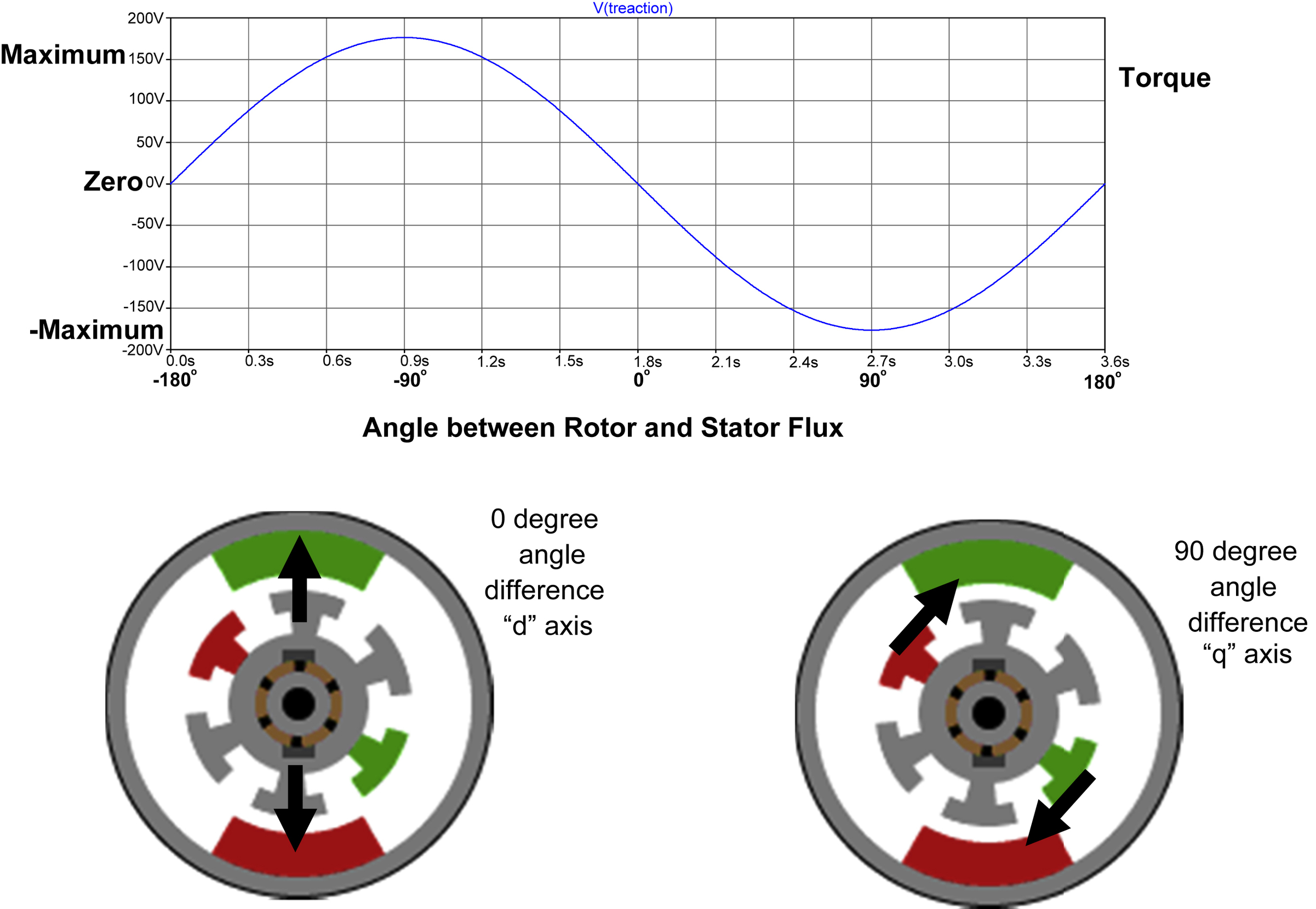
First consider the PMAC motor. The goal of the controller is to maintain either the axis of the PM rotor magnets or the induced magnetic field of the rotor at 90 degrees (plus or minus depending on the direction of rotation) with respect to the angle of the stator flux, under varying motor speed and load. When the stator flux is at 90 degrees to the rotor, this is called the quadrature direction or “q.” When the stator flux is at 0 degrees to the rotor, this is called the direct direction or “q”. As these d and q are orthogonal, the relative angle between the rotor and stator can be described in terms of d and q components. With a permanent magnet, the rotor flux angle is known as long as the rotor position can be determined. Then the AC stator currents can be driven such that the stator flux vector is maintained at 90 degrees with respect to the rotor flux. This is a dynamic procedure, as the motor is spinning and the both the d- and q-axis are spinning. To simplify the controller design, a pair of transforms is used, known as the “Clark” and “Park” transform.
14.7. Park and Clark Transforms
Most AC motors are three phase, with each stator coil wound at 120 degrees relative to each other. Each of these currents creates a magnetic flux vector. These vectors will sum up to produce a net vector, which is rotating. Describing the net vector in terms of three components is inconvenient. The Clark transform solves this, by mapping the stator flex vector from three components A, B, and C of 120 degrees separation into two orthogonal components, α and β (Fig. 14.18).
The Clark transform equations are defined as follows:
The Clark transform is reversible, and the inverse Clark transform equations are as follows:
The control loop processing will be done by using the two orthogonal axis, α and β. The feedback current measurements of the motor will use the Clark transform to generate the Iα and Iβ. The output of the control loop processing will use the inverse Clark transform to translate back into the three phase currents IA, IB,, and IC to be generated by the invertor.
Another transform is used, the Park transform. The currents are rotating at a synchronous rate with the rotor in a PMAC motor. However, the control loop operates at much lower frequencies. The Park transform uses the rotor angular position θ and by calculating continuously is able to remove the rotation of the currents. Recall that the goal of control loop is to adjust the relative phase or phase difference between the stator magnetic flux and the magnetic flux of the rotor.

The Park transform equations are defined as follows:
And the inverse Park transform equations are as follows:
The Park transform is shown pictorially above. To summarize, the three phase rotating currents are described in terms of three axes at 120 degrees (A, B, C). The currents first mapped into two orthogonal components (α, β) using two orthogonal axis at 90 degrees, using the Clark transform. Then, as the rotor angle θ (and therefore rotor flux vector direction) is known, the stator flex vector is then mapped into two other orthogonal current vectors (d, q), using the Park transform. If this was a static situation (the rotor not rotating, the stator currents not rotating), then this would be insignificant. However, the Park transform is computed continually, with update rotor angle θ. This means that d and q orthogonal vectors are rotating along with the rotor. The d-axis by definition is in the same direction as the rotor magnetic flux. The Park transform has mapped the stator currents into two components: a “d” component, which creates a magnetic flux in such a direction as to create zero torque on the rotor, and a “q” component, which will create maximum torque on the rotor. In a system where the motor is running at constant speed at a constant load (torque), the “d” and “q” components will be static or DC values will be static. During motor operation, with the d- and q-axis spinning, stator currents are continually updated as to drive the stator flux pattern to be offset by 90 degrees from the d-axis. So while the Iα and Iβ values change in a sinusoidal manner, the Id and Iq values are DC (or near DC). The Id and Iq current vectors change only in response to a change in motor operation. For example, when the motor load increases or there is an external command to increase speed, more torque will be required. This requires an increase in magnetic stator flux intensity, by increasing stator current levels (which would make the current vectors longer in Fig. 14.19) longer. Note that Fig. 14.19 is three dimensional, and “C” is coming out of the page. The goal of the control loop is to maintain the stator flux vector at 90 degrees with respect to the rotor flux vector, which is done by making the “d” component to zero, and “q” to such a value as to create the amount of torque to drive the motor at the desired rotational speed.

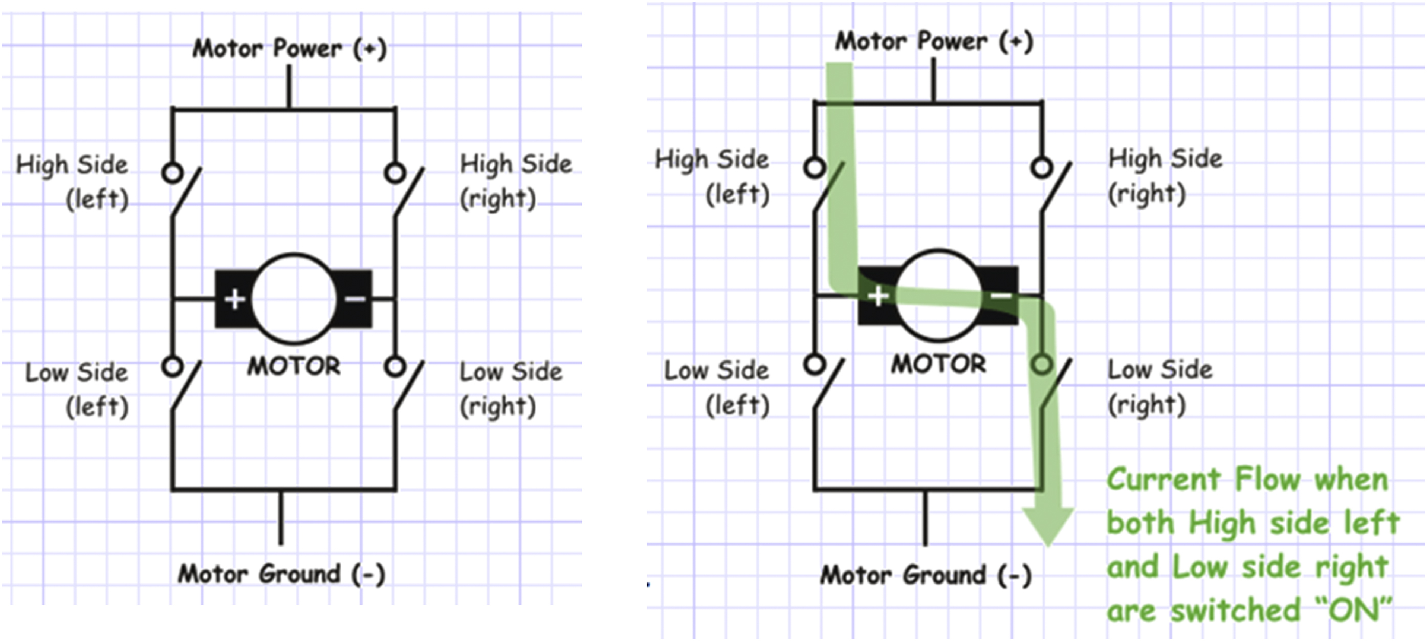
To review, the inverse Clark transform is used to take the control loop outputs in the form of orthogonal Id and Iq current values, and transform them into orthogonal rotating Iα and Iβ waveforms. The inverse Park transform is used to then map Iα and Iβ signals into three phase IA, IB, and IC s waveforms, which then drive the inverter that creates the actual motor currents using “H” bridge circuits with PWM modulation. Control loops operate from an error signal or the difference between the actual and desired values. The control loops that control the torque (or motor stator current) for “d” and “q” need the actual values. This is done by measuring the actual motor currents, which can be accomplished by using “sense” resistors or more advanced inductive current sensors. In either case, the currents measured are the actual IA, IB, and IC currents. The three phase signals are then mapped to Iα and Iβ signals using the Clark transform. Then the Iα and Iβ signals are in turn mapped to Id and Iq signals using the Park transform. The Id signal should be driven to zero in a permanent magnet synchronous motor (PMSM), and so is subtracted from zero to form the error signal into the P and I control circuits for the direct current vector. The Iq vector is proportional to torque. Therefore, the desired torque level (which is often the output of a velocity control loop) is subtracted from the actual, measured Iq signal to form the error signal into the P and I control circuits for the quadrature current vector. Note that the rotor position is a required input for Park and inverse Park transform computations. The whole point of the Park and Clark transforms is to remove the high frequency, rotational commutation from the control loop, and to separate our the direct and quadrature components so each can be independently controlled.
The ACIM can be controlled in a very similar manner as the PMSM. However, the feedback rotor position θd must be modified to introduce the slip frequency into the control circuits (keep in mind that just as velocity is the derivative of position, the rotational speed is the derivative of the rotational angle position θd). By adding (or subtracting) an angular offset to each successive rotor position sample, an increase (or decrease) in frequency is affected. For an ACIM, the slip is proportional to the torque. Therefore a slip controller calculator is needed. The controller will attempt to drive the ACIM at the desired speed. However, when the ACIM is running at a lower speed, more torque is needed to achieve the speed increase. This is achieved by having the slip calculator add phase offsets to achieve a faster effective frequency across the θd sample train, which will result in a higher frequency stator commutation, which allows the ACIM to slip and still run at the desired input frequency. This will in effect change the phase of the combined Id and Iq vectors to advance faster than the rotor rotation. The control loops will also increase the vector length of Id and Iq, to achieve greater torque, until the desired speed is achieved (Fig. 14. 20).

In summary, an ACIM motor can be driven directly from an AC power source, but it will not run synchronously, as greater loads result in greater slip. Since the AC voltage source is generally fixed, the curve of motor torque verses rotational speed is also fixed. This works well for many applications where the load is known, and the motor operational speed is within a fixed range.
The ACIM can also be electronically commutated and controlled from a DC source, in which case the motor speed and operational profile can be controlled under varying load conditions. The motor can also be easily reversed in rotational direction.
..................Content has been hidden....................
You can't read the all page of ebook, please click here login for view all page.