Chapter 4
Frequency Response
Abstract
A discussion has been made on a frequency response where digital signal processing is performed. The goal to modify the frequency representation of a signal through filtering is the most elemental signal processing functions. Gradually, the discussion moves toward the responses and the complex exponential factors affecting it. It also touches on how to use a filter to normalize the response, when an input frequency is put through. The chapter also uses digital filter as a linear device to change the amplitude and phase of the input signal.
Keywords
Complex exponential; Digital signal processing; Frequency response; Passband; Touch tone frequencies
Once we have a sampled digital signal, we are ready to perform digital signal processing (DSP) on this signal. In the last chapter, we briefly touched on representing the signal in the frequency domain. Usually, our goal is to modify the signal's frequency representation. This is normally performed using a filtering function. This is probably the most fundamental of DSP functions. In the previous example of the telephone system, we talked about sampling the voice signal at 8 kHz. Let us say we want to build an automated system to detect touch tones (on a touch tone phone, whenever you press a number key, the phone creates two specific tones or frequencies in the audio signal band—which is what you hear when pressing the button). We could build a digital filter for each of the possible tones, feed the sampled audio signal into each filter, and monitor the outputs of the filters. In this way, we could detect when the telephone user presses the buttons, and which button was pressed, which is exactly what touch tone phone systems do.
4.1. Frequency Response and the Complex Exponential
In this chapter, we need to understand the concept of frequency response. Then in the next chapter, we will develop a way to relate a filter's frequency and time response. First, let us begin with an intuitive way to understand the frequency response of a filter. From the last chapter, we learned that we can create a complex exponential signal, which is just a positive or negative frequency rotation about the unit circle (radius = 1). Furthermore, when the frequency of the complex exponential reaches the Nyquist frequency, we have reached the maximum frequency that can be represented for a given sampling rate.
A complex exponential signal has the following forms:
This is very similar to what we saw before. The earlier angle Ω has been replaced by ωt or by 2πft. The significance of this is that we are no longer representing a point or vector on the unit circle of the complex number plane (as determined by angle Ω). Now we are representing a time-varying signal. This signal will move about the unit circle with a rotational speed of ω radians per second. For a given ω (rotational speed), we can determine the position of the signal at any given point in time (denoted by “t”).
The second equation is equivalent to the first, except the rotational speed is expressed in cycles (revolutions) per second, denoted by “f”. Try to make sure this is clear before moving on, because both forms will appear interchangeably in the DSP world.
t represents time, in seconds.
ω represents rotational speed, in radians per second (2π radians = one revolution).
f represents rotational speed, in cycles (or revolutions) per second.
The variables ω and f simply describe the same thing, using different units, like inches and centimeters. Recall from before that it takes exactly 2π radians to complete a full circle. So 1 cycle per second equals 2π radians per second, or ω = 2πf.
Both ω and f denote the rotational speed in the counterclockwise direction. A negative value for ω or f means we are rotating in the opposite direction (clockwise). Let us now consider an example. Let the rotational speed equal to 1/8 of a circle per second (takes 8 s to complete one revolution). Therefore, f = 1/8. Also, ω = 2πf, or ω = π/4. This signal (let us call it “s”) can be described as:
We can evaluate s(t) at any given time t. For example, refer to Table 4.1:
We can also plot s(t). Shown in Fig. 4.1 are of separate plots of the real (dotted line) part of s(t) and the imaginary (dashed line) part of s(t). Also shown in Fig. 4.2, in on a separate plot is the complete signal s(t) on the unit circle of the complex number plane with time labels at each point.
4.2. Normalizing Frequency Response
Notice that we are measuring the value of our signal once per second. It turns out that it is often convenient to set the sampling frequency Fs equal to 1 s. This is called normalization. The frequency response of a filter can be expressed as a normalized response, where the input frequency is expressed as a fraction of sampling frequency Fs. Let us illustrate this using the telephone system as an example. In this case, Fs = 8000 Hz, FNyquist = 4000 Hz, and one of the touch tones we need to detect is at 770 Hz. We could build a filter with a passband (portion of frequency band to “pass through” the signal, with minimum attenuation) to detect 770 Hz. Since we need a little tolerance, lets decide to make the passband from 760 to 780 Hz and our desired stopbands (portion of frequency band to “stop” or block the signal, with maximum attenuation) is from 0 to 760 and from 780 to 4000 Hz (recall FNyquist = Fs/2). Do not forget that we are assuming no signal at frequencies above FNyquist, this has been already taken care of before sampling. This could also be expressed as a passband from 0.0950 to 0.0975 Fs, and stopbands from 0 to 0.0950 Fs and from 0.0975 to Fs/2. All these frequencies have been normalized, by dividing with our Fs = 8000 Hz. When designing a digital filter, it is common to normalize the frequency response in terms of Fs (Table 4.2).
Table 4.1
Rotational Representations of s(t)
| Time t in Seconds | s(t) = ejπt/4 | Angle of s(t) in Degrees | Angle of s(t) in Radians |
| 0 | 1 | 0 | 0 |
| 1 | 0.707 + 0.707 j | 45 | π/4 |
| 2 | J | 90 | π/2 |
| 3 | −0.707 + 0.707 j | 135 | 3π/4 |
| 4 | −1 | 180 | π |
| 5 | −0.707–0.707 j | 225 | 5π/4 = −3π/4 |
| 6 | −j | 270 | 3π/2 = −π/2 |
| 7 | 0.707–0.707 j | 315 | 7π/8 = −π/4 |
| 8 | 1 | 360 = 0 | 2π = 0 |


Table 4.2
| Touch Tone Bandpass Detection Filter Example | Actual Frequency (Hz) | Normalized Frequency (Fs = 8000 Hz) |
| Touch Tone Frequency | 770 | 0.09625 Fs (770/8000) |
| Start of Passband | 760 | 0.0950 Fs (760/8000) |
| End of Passband | 780 | 0.0975 Fs (780/8000) |
| Nyquist Frequency | 4000 | 0.50 Fs (4000/8000) |
Now let us get back to frequency response. Suppose we take our filter, and input a series of complex exponential signals into the filter. Each exponential will be a little higher frequency than the previous. We check the output of each frequency. What we will find is if we input a complex exponential of a given frequency, we will see at the output a complex exponential signal of the same frequency. That is because a digital filter is a linear device, so it cannot create new frequencies, or change the frequency of a signal passing through it. What it can do is to change the amplitude and phase of the input signal. Let us leave the phase part out of it for now, and focus on the amplitude.
4.3. Sweeping Across the Frequency Response
Suppose we build a digital signal generator that can create a complex exponential signal of any frequency we desire, from 0 to FNyquist (this is called a numerically controlled oscillator or NCO, and it is common in digital communication systems). We drive our filter with the NCO, incrementing the frequency in small steps, and we measure the amplitude of the filter output signal. If we plot this data, we will have the magnitude response of our filter with all frequencies from 0 to FNyquist.
If we do this for the touch tone filter above, we will get zero output until we input a complex exponential at frequency 0.0950 Fs. From frequency 0.0950 Fs until 0.0975 Fs, the complex exponential will pass through our filter, and could be detected. Above 0.0975 Fs up until FNyquist, we will get zero output. This type of filter is called a bandpass filter, because it allows only a portion of the frequency band to pass and blocks frequencies above and below this band.
Now remember, we can also have negative frequency complex exponentials, so we could also do a similar plot from 0 to −FNyquist. For the vast majority of digital filters, the frequency response will be the same whether the input is positive or negative frequency. All filters with real (as opposed to complex) coefficients will have this property.
Referencing everything to Fs is also convenient when using our NCO. The NCO does not know that it is being clocked at 8 kHz sampling frequency. Instead when we program it, we need to set the desired frequency output in terms of Fs. For example, to test our filter with an input of 770 Hz, we need the NCO to produce a complex exponential at 0.09,625 Fs or (770/8000) Fs.
4.4. Example Frequency Responses
After this long winded explanation, let us show some examples of frequency responses to help clarify things. In this chapter, we will depict the frequency response of ideal filters. First we will show low pass, then high pass, and lastly a bandpass, like our touch tone 770 Hz detector.
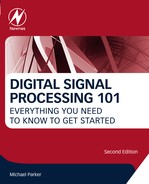
Please note that the filter response repeats at intervals of Fs. This is an artifact of sampling, as explained in the last chapter. The valid portion of the sampled frequency response is from −FNyquist to + FNyquist. Just as we saw the apparent rate of rotation of the wheel with the red dot reach a maximum at a rate of ½ the sample rate, and then slowly decrease until it finally stopped when the rate of rotation equaled the sample rate, the frequency response of the filter will behave similarly between zero and Fs. So the filter response near zero will be the same as that near Fs and the filter response just below FNyquist will be the same as just above FNyquist. In fact, since this phenomenon is well understood, there is really no reason to plot a digital filter's response above FNyquist and below −FNyquist. We are doing it here in Fig. 4.3 mainly to show this point.

The low pass filter passes frequencies near zero. Both positive and negative frequencies are passed. When the frequency reaches the chosen Fcutoff, the filter no longer passes the signal. As we approach any multiple of Fs, we see the aliasing of the filter response, in Fig. 4.4.
Here in Fig. 4.4 we gradually reduced the low pass filter response as it approaches Fcutoff. This is to show that it is possible to design for an arbitrary passband response, and a gradual transition to the stopband, not just a flat response in the filter passband with an abrupt transition at Fcutoff.
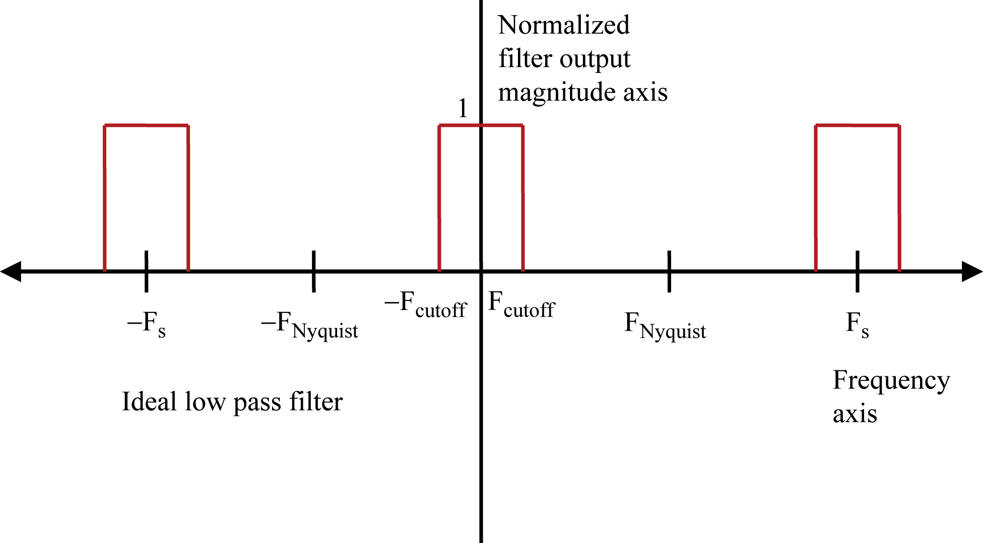
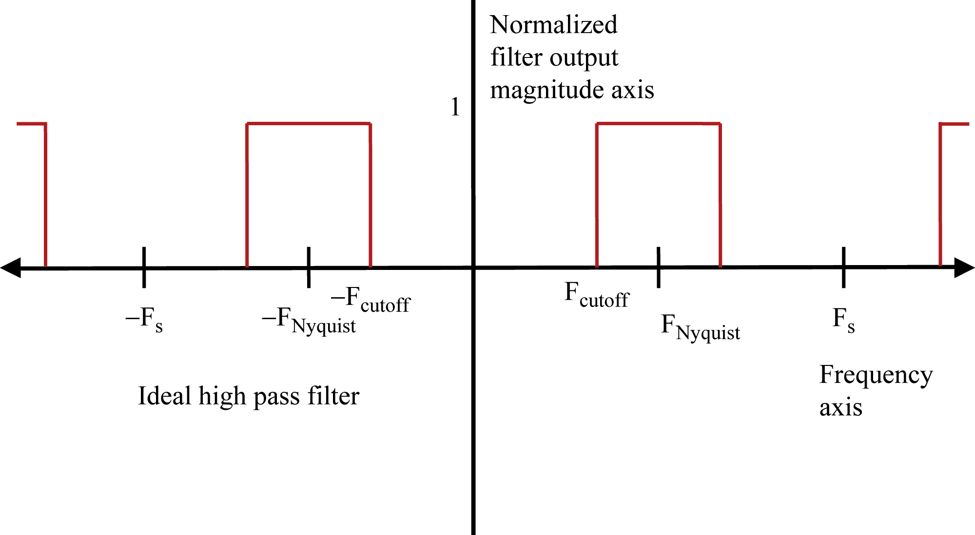
The high pass filter in Fig. 4.5 passes frequencies near FNyquist. Both positive and negative frequencies are passed. When the frequency falls below Fcutoff, the filter no longer passes the signal. Aliasing is again seen by the symmetry about FNyquist.

Bandpass (do not confuse this with the early term “passband”) filters pass only a specific band, or portion of frequencies, which does not include either DC (0 Hz) or FNyquist. The band-pass filter in Fig. 4.6 again shows the alias effect. This repeats to infinity at every multiple of Fs. Going back to Fig. 4.3, the low pass filter frequency plot, we see the alias centered at Fs. So according to our plot, the filter will pass frequencies around Fs, even though this is above our Fcutoff. So if we input a signal near Fs to an ADC, it will appear as a frequency near zero, and be passed by our filter.
This is a difficult concept, which is why there is so much repetition on this theme. Do not be worried if you have to go back and forth a few times to the diagrams or earlier chapters to really satisfy yourself that you understand it. It is a key concept for much of what follows, and unfortunately, there are some experienced people working in DSP industry who still have trouble with these fundamentals.
4.5. Linear Phase Response
Earlier, we decided to ignore the phase response. We are just concerned with the magnitude response (remember that complex numbers have both a magnitude and phase). This is because, for most filters, the phase response is not something we need to worry about. The most common type of digital filter is called the finite impulse response, or FIR, and it has what is called a linear phase response. This means that every frequency passing through the filter experiences the same delay, which works out to a linearly increasing phase as the frequency increases. This sounds complicated, but the short story is that for FIR filters, we do not need to worry about phase response. This is the type of filter we will discuss in detail in the next chapter and is the most common DSP function implemented.
4.6. Normalized Frequency Response Plots
Now we have one more topic to finish out this chapter. We now know that it is sufficient to describe a digital filter response from −FNyquist to + FNyquist. But frequently, in textbooks or filter design programs, the frequency response will be given in terms of normalized radians per second, ω, rather than normalized frequency, as shown in Fig. 4.7.
Again, let us refer back to our complex exponential, ejωt. We are sampling at a normalized frequency of 1 sample per second, or 2π radians per second. That means that a complex exponential of frequency π radians per second will correspond to FNyquist and 2π radians per second will correspond to Fs. This is exactly what we see when we plot the frequency response using the ω axis.
As a review, see Table 4.3 providing example low pass response cutoff both in terms of ω and Fs. It is important to be comfortable going between these two representations, because most filter design programs are defined in terms of ω, but to design your filter, you need to be able to translate to the real frequencies used in your application to the filter response in terms of ω.

Table 4.3
| % of Maximum Possible Low Pass Filter Bandwidth (%) | Ω (Radians per Second) | Fs (Hz or Cycles per Second) |
| 10 | π/10 | Fs/20 |
| 10 | −π/10 | −Fs/20 |
| 25 | π/4 | Fs/8 |
| 50 | π/2 | Fs/4 |
| 80 | 4π/5 | 2Fs/5 |
| 100 | π | Fs/2 or FNyquist |
The cutoff point is defined as a percentage of the maximum bandwidth possible for a low pass filter, with 100% becoming an all-pass filter (every frequency passes through). Normally, the filter frequency response will be symmetric, so Fcutoff = −Fcutoff.
..................Content has been hidden....................
You can't read the all page of ebook, please click here login for view all page.