
Chapter 25
Image and Video Compression Fundamentals
Abstract
Now that we have the basics of entropy, predictive coding, DCT, and quantization, we are ready to discuss image compression. Image compression, in contrast to video compression, deals with a still image, rather than a continuous sequence of images, which makes up a video stream. Following that, the basics of video compression are discussed. Video is made up of a stream of images, which can have high degrees of correlation that can be exploited to reduce the amount of data needed to transmit the video stream. Both image and video compression are lossy processes, which mean that information is permanently lost in the compression process.
Keywords
AC coefficients; B frames; Baseline JPEG; DC coefficient; GOP; Huffman coding; I frames; Intercoded; Intracoded; JPEG; Lossy compression; Macrocell block; MAD; MMSE; Mquant; P frames; Residual; Slice; VBV
Now that we have the basics of entropy, predictive coding, DCT, and quantization, we are ready to discuss image compression. Image compression, in contrast to video compression, deals with a still image, rather than a continuous sequence of images, which makes up a video stream.
JPEG is often ubiquitous with image compression. JPEG stands for Joint Photographic Experts Group, a committee that has published international standards on image compression. JPEG is an extensive portfolio of both lossy and lossless image compression standards and options. In this section, we will focus on baseline JPEG.
25.1. Baseline JPEG
With baseline JPEG, each color plane is compressed independently. A monochrome image would have 8 bits per pixel. Generally, lossy compression can achieve less than 1 bit on average per pixel with high quality.
For RGB images, each of the three color planes is treated independently. With YCrCb representation, Y, Cr, and Cb are treated independently. For 4:2:2 or 4:2:0 YCrCb, the Cr and Cb are undersampled, and these undersampled color planes will be compressed. For example, standard definition images are 720 (width) by 480 (height) pixels. For 4:2:2 YCrCb representation, the Cr and Cb planes will be 360 by 480 pixels. Therefore, a higher degree of compression can be achieved using JPEG on 4:2:2 or 4:2:0 YCrCb images. Intuitively, this makes sense, as more bits are used to represent the luminance to which the human eye is more sensitive and less to the chrominance to which the human eye is less sensitive.
25.2. DC Scaling
Each color plane of the image is divided up into 8 × 8 pixel blocks. Each 8-bit pixel can have a value ranging from 0 to 255. The next step is to subtract 128 from all 64 pixel values, so the new range is −128 to +127. The 8 × 8 DCT is next applied to this set of 64 pixels. The DCT output is the frequency domain representation of the image block.
The upper left DCT output is the DC value, or average of all the 64 pixels. Since we subtracted 128 prior to the DCT processing, the DC value can range from −1024 to 1016, which can be represented by an 11-bit signed number. Without the 128 offset, the DC coefficient would range from 0 to 2040, while other 63 of the DCT coefficients would be signed (due to the cosine range). The subtraction of 128 from the pixel block has no effect on the 63 AC coefficients (an equivalent method could be to perform subtraction of −1024 of DC coefficient after the DCT).
25.3. Quantization Tables
The quantization table used has a great influence on the quality of JPEG compression. It also influences the degree of compression achieved. These tables are often developed empirically (by trial and error) to give the greatest number of bits to the DCT values, which are most noticeable and have the most impact to the human vision system.
The quantization table is applied to the output of the DCT, which is an 8 × 8 array. The upper left coefficient is the DC coefficient, and the remaining are the 63 AC coefficients, of increasing horizontal and vertical frequencies as one moves rightward and downward. As the human eye is more sensitive to lower frequencies, less quantization and more bits are used for the upper and leftmost DCT coefficients which contain the lower frequencies in vertical and horizontal directions.
Example baseline tables are provided in the JPEG standard, as shown below.
| Luminance Quantization Table of Q j,k values | |||||||
| 16 | 11 | 10 | 16 | 24 | 40 | 51 | 61 |
| 12 | 12 | 14 | 19 | 26 | 58 | 60 | 55 |
| 14 | 13 | 16 | 24 | 40 | 57 | 69 | 56 |
| 14 | 17 | 22 | 29 | 51 | 87 | 80 | 62 |
| 18 | 22 | 37 | 56 | 68 | 109 | 103 | 77 |
| 24 | 35 | 55 | 64 | 81 | 104 | 113 | 92 |
| 49 | 64 | 78 | 87 | 103 | 121 | 120 | 101 |
| 72 | 92 | 95 | 98 | 112 | 100 | 103 | 99 |
| Chrominance Quantization Table of Q j,k values | |||||||
| 17 | 18 | 24 | 47 | 99 | 99 | 99 | 99 |
| 18 | 21 | 26 | 66 | 99 | 99 | 99 | 99 |
| 24 | 26 | 56 | 99 | 99 | 99 | 99 | 99 |
| 47 | 66 | 99 | 99 | 99 | 99 | 99 | 99 |
| 99 | 99 | 99 | 99 | 99 | 99 | 99 | 99 |
| 99 | 99 | 99 | 99 | 99 | 99 | 99 | 99 |
| 99 | 99 | 99 | 99 | 99 | 99 | 99 | 99 |
| 99 | 99 | 99 | 99 | 99 | 99 | 99 | 99 |

Many other quantization tables claiming greater optimization to the human visual system have been developed for various JPEG versions.
The quantized output array is formed as follows:
where Aj,k is the DCT output array value, Qj,k is the quantization table value.
A couple of examples would be:
When the quantization values Q j,k are large, this results in few possible values of the output Bj,k. For example, with a quantization value of 99, the rounded output values can only be −1, 0, or +1. In many cases, especially when j or k is 3 or larger, the Bj,k will be rounded to zero, indicating little high frequency in the image region.
This is lossy compression. Data are lost in quantization and cannot be recovered. The principle is to reduce the data by discarding only data that have little noticable impact on the image quality.
25.4. Entropy Coding
The next step is to sequence the quantized array values Bj,k as in the order shown in Fig. 25.1. The first value B0,0 is the quantized DC coefficient. All the subsequent values are AC values.

The entropy encoding scheme is fairly complex. The AC coefficients are coded differently than that of the DC coefficient. The output of the quantizer often contains many zeros, so special symbols are provided. One is an EOB of end of block symbol, used when the remaining values from the quantizer are all zero. This allows the encoding to be terminated when the rest of the quantized values are zero. The coded symbols also include ability to specify the zero run length following a nonzero symbol, again to help efficiently take advantage of the zeros present within the quantizer output. This is known as run length encoding.
The DC coefficients are differentially coded across the image blocks. There is no relationship between the DC and AC coefficients. However, DC coefficients in different blocks are likely to be correlated, as adjacent 8 × 8 image blocks are likely to have a similar DC or average luminance and chrominance across nearby image blocks. So the only difference is coded for the next DC coefficient, relative to the previous DC coefficient.
Four Huffman code tables are provided in the baseline JPEG standard:
• DC coefficient, luminance,
• AC coefficients, luminance,
• DC coefficient, chrominance,
• AC coefficients, chrominance.
These tables give encoding for both individual values, and values plus a given number of zeros. Following the properties of Huffman coding, the tables are constructed so that the most statistically common input values are coded using the fewest number of bits. The Huffman symbols are then concatenated into a bitstream, which forms the compressed image file. The use of variable length coding makes recovery difficult if any data corruption occurs. Therefore, special symbols or markers are inserted periodically to allow the decoder to resynchronize in the event of any bit errors in the JPEG file.
The JPEG standard specifies the details of the entropy encoding followed by Huffman coding. It is quite detailed and is not included in this text. For nonbaseline JPEG, alternate coding schemes may be used.
For those planning to implement a JPEG encoder or decoder, the following book is recommended: JPEG Digital Image Compression Standard, by William Pennebaker and Joan Mitchell.
We have described the various steps in JPEG encoding. The Baseline JPEG process can be summarized by the following encode and decode steps, as shown in Fig. 25.2.

25.5. JPEG Extensions
The JPEG standard provides several extensions, some of which are summarized below.
Huffman coding is popular and has no intellectual property restrictions. However, some variants of JPEG use an alternate coding method known as arithmetic coding. Arithmetic coding is more efficient and will adapt to changes in the statistical estimates of the input data stream, and it is subject to patent limitations.
Variable quantization is an enhancement to the quantization procedure of DCT output. This enhancement can be used with the DCTs in JPEG except for the baseline JPEG. The quantization values can be redefined prior to the start of an image scan but must not be changed once they are within a scan.
With variable quantization, the quantization values are scaled at the start of each 8 × 8 block, but matching the scale factors used to the AC coefficients stored in the compressed data. Quantization values may then be located and changed as needed. This provides for variable quantization based on the characteristics of an image. The variable quantizer continually adjusts during decoding to provide higher quality at the expense of increasing the size of the JPEG file. Conversely, the maximum size of the resulting JPEG file can be set by constant adaptive adjustments made by the variable quantizer.
Another extension is selective refinement, which selects a given region of an image for further enhancement. The resolution of the region of an image is improved using three methods of selective refinement: progressive, hierarchical, and component.
Progressive selective refinement is used only in the progressive modes to add more bit resolution of near zero and nonzero DCT coefficients in region of the image. Hierarchical selective refinement is used in JPEG hierarchical coding mode and permits for a region of an image to be refined by the next differential image in a defined hierarchical sequence. It allows higher quality or resolution in a given region of the image. Component selective refinement permits a region of a frame to contain fewer colors than are originally defined.
Image tiling is an enhancement to divide a single image into smaller subimages, which allows for smaller memory buffers, quicker access in both volatile and disk memory, and the storing and compression of very large images. There are three types of tiling: simple, pyramidal, and composite.
Simple tiling divides an image in multiple fixed-size tiles. All simple tiles are coded from top to bottom, left to right, and are adjacent. The tiles are all the same size, and encoded using the same procedure.
Pyramidal tiling also partitions the image into multiple tiles, but each tile can have different levels of resolution. This is known as the JPEG Tiled Image Pyramid (JTIP) model, resulting in a multiresolution pyramidal JPEG image. The JTIP image has successive layers of the same image but using different resolutions. The top of the pyramid has an image that is 1/16th of the defined screen size. It is called the vignette that can be for quick displays of image contents. The next image is one-fourth of the screen and is called the imagette. This is often used to display multiple images simultaneously. Then comes is a lower-resolution, full-screen image. After that are higher-resolution images. The last is the original image. Each of the pyramidal images can be JPEG encoded, either separately or together in the same data stream. If done separately, then it can allow for faster access of the selected image quality.
Multiple-resolution versions of images can also be stored and displayed using composite tiling known as a mosaic. The difference from pyramidal tiling is that composite tiling permits the tiles to overlap, be different sized, and be encoded using different quantization scaling. Each tile is encoded independently, so they can be easily combined.
25.6. Video Compression Basics
MPEG is often considered ubiquitous with image compression. MPEG actually stands for Moving Pictures Experts Group, a committee which publishes international standards on video compression. MPEG is a portfolio of video compression standards, which will be discussed further in the next chapter.
Image compression theory and implementation focus on taking the advantage of the spatial redundancy present in the image. Video is composed of a series of images, usually referred to as frames, and so can be compressed by compressing the individual frames as discussed in the last chapter. However, there are temporal (or across time) redundancies present across video frames. This means that the frame immediately following has a lot in common with the current and previous frames. In most videos, there will be a significant amount of repetition in the sequences of frames. This property can be used to reduce the amount of data used to represent and store a video sequence. To take advantage of the temporal redundancy, this commonality must be determined across the frames.
This is known as predictive coding and is effective to reduce the amount of data that must be stored or streamed for a given video sequence. Usually, only parts of the image changes from frame to frame, which permits prediction from previous frames. Motion compensation is used in the predictive process. If an image sequence contains moving objects, then the motion of these objects within the scene can be measured, and the information used to predict the location of the object in frames later in the sequence.
Unfortunately, this is not as simple as just comparing regions in one frame to another. If the background is constant, and objects move in the foreground, there will be significant areas of the frames that will not change. But if the camera is panning across a scene, then there will be areas of subsequent frames that will be the same, but will be shifted in location from frame to frame. One way to measure this is to sum up all the absolute differences (without regard to sign), pixel by pixel, between two frames. Then the frame can be offset by one or more pixels and the same comparison run. After many such comparisons, the sum of differences results can be compared, and the minimum result corresponds to the best match. This will provide for a method to determine the location offset of the match between frames. This is known as the minimum absolute differences (MAD) method, or sometime referred to as sum of absolute differences (SAD). An alternative is the minimum mean square error (MMSE) method that measures the sum of the squared pixel differences. This method can be useful because it accentuates large differences, due to the squaring, but the trade-off is it requires multiplies in addition to subtractions.
25.7. Block Size
A practical trade-off is determining the block size to run the comparison over. When the block size is too small, there is no benefit in trying to reuse pixel data from a previous frame rather than just use the current frame data. If the block is too large, there will be many more differences likely and is difficult to get a close match. One obvious block size to run comparisons across would be the 8 × 8 block size used for DCT. Experimentation has shown that a 16 × 16 pixel area works well, and this is commonly used. This size is referred to as a “macroblock.”
The computational effort to run these comparisons can be enormous. For each macroblock, 256 pixels must be compared against a 16 × 16 area of the previous frame. If we assume the macroblock data could shift by up to, say, 256 pixels horizontally or 128 pixels vertically (a portion of an HD 1080 × 1920) from one frame to another, there will be 256 possible shifts to each side and 128 possible shifts up or down. This is a total of 512 × 256 = 131,072 permutations to check, each requiring 256 difference computations. This is over 33 million per macroblock, with 1080/16 × 1920/16 = 8100 macroblocks per HD image or frame (Fig. 25.3).
25.8. Motion Estimation
However, there are methods to reduce this brute force method. A larger block size can be used initially, over larger portions of the image, to estimate the motion trend between frames. For example, enlarging the block size to include macrocells on all sides, for a 48 × 48 pixel region, can be used for motion estimation. Once the motion estimation is completed, this can be used to dramatically narrow down the number of permutations to perform the MAD or MMSE over. This motion estimation process is normally performed using luminary (Y) data. Also, motion estimation is performed locally for each region. The case of the camera panning will move large portions of an image with a common motion vector, but in cases with moving objects within the video sequence, different objects or regions will have different motion vectors.
Note that these motion estimation issues are present only on the encoder side. The decoder side is much simpler, as it must recreate the image frames based on data supplies in compressed form. This asymmetry is common in audio, image, video, or general data compression algorithms. The encoder must search for the redundancy present in the input data using some iterative method, whereas the decoder does not require this functionality (Fig. 25.4).
Once a good match is found, the macroblocks in the following frame data can be minimized during compression by referencing the macroblocks in previous frames. However, even a “good” match will have some error. That is referred to a residuals or residual artifacts. These artifacts can be determined by differences in the four 8 × 8 DCTs in the macroblock. These differences can be coded and compressed as part of the frame data. Of course, if the residual is too large, coding the residual might require more data compared to just compressing the image data without any reference to the previous frame.


For MPEG compression, the source video is first converted to 4:2:0 format, so the chrominance data frame is one-fourth the number of pixels, ½ vertical and ½ horizontal resolution. The video must be in progressive mode; that is, each frame is composed of pixels all from the same time instant (that is, not interlaced).
At this point, a bit of terminology and hierarchy used in video compression needs to be introduced.
• A pixel block refers to an 8 × 8 array in a frame.
• A macrocell is 4 blocks, making a 16 × 16 array in a frame.
• A slice is a sequence of adjacent macrocells in a frame. If data are corrupted, the decoding can typically begin again at the next slice boundary.
• A group of pictures (GOP) is from one to several frames. The significance of the GOP is that it is self-contained for compression purposes. No frame within one GOP uses data from a frame in another GOP for compression or decompression. Therefore, each GOP must begin with an I frame (defined below).
• A video is made up of a sequence of GOPs.
Most video compression algorithms have three types of frames:
• I frames—These are frames which are compressed using only information in the current frame. The video compression term for this is intracoded, meaning the coding uses information within the frame only. A GOP always begins with an I frame, and no previous frame information is required to compress or decompress an I frame.
• P frames—These are predicted frames. P frames are compressed using image data from an I or P frame (may not be the immediate preceding frame) and comparing to the current P frame. Restoring or decompressing the frame requires compressed data from a previous I or P frame plus residual data and motion estimation corresponding to the current P frame are used. The video compression term for this is intercoded, meaning the coding uses information across multiple video frames.
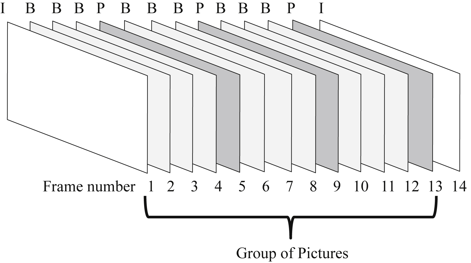
• B frames—These are bidirectional frames. B frames are compressed using image data from proceeding and following I or P frames. This is compared to the current B from a data to form the motion estimation and residuals. Restoring or decompressing the B frame requires compressed data from proceeding and following I or P frames plus residual data and motion estimation corresponding to the current B frame are used. B frames are intercoded (Fig. 25.5).
Also, by finishing the GOP with a P frame, the last few B frames can be decoded without needing information from the I frame of the following GOP.
25.9. Frame Processing Order
The order of frame encode processing is not sequential. Forward and backward prediction mean that each frame has a specific dependency that mandates processing order and requires buffering of the video frames to allow out-of-sequential order processing. This also introduces multiframe latency in the encoding and decoding process.
At the start of the GOP, the I frame is processed first. Then the next P frame is processed, as it needs current frame plus information from the previous I or P frame. Then the B frames in between are processed, as in addition to the current frame, information from both previous and postframes are used. Then the next P frame, and after that the intervening B frames, as shown in the processing order given in Fig. 25.6.
Note that since this GOP begins with an I frame and finishes with a P frame, it is completely self-contained, which is advantageous when there is data corruption during playback or decoding. A given corrupted frame can only impact one GOP. The following GOP, since it begins with an I frame, is independent of problems in a previous GOP.

25.10. Compressing I Frames
I frames are compressed in very similar fashion using the JPEG techniques covered in the last chapter. The DCT is used to transform pixel blocks into the frequency domain, after which quantization and entropy coding is performed. I frames do not use information in any other video frame, therefore an I frame is compressed and decompressed independently from other frames. Both the luminance and chrominance are compressed, separately. Since 4:2:0 format is used, the chrominance will have only ¼ as many macrocells as the luminance. The quantization table used is given below. Notice how again larger amounts of quantization are used for higher horizontal and vertical frequencies, as the human vision is less sensitive to high frequency.
| Luminance and Chrominance Quantization Table | |||||||
| 8 | 16 | 19 | 22 | 26 | 27 | 29 | 34 |
| 16 | 16 | 22 | 24 | 27 | 29 | 34 | 37 |
| 19 | 22 | 26 | 27 | 29 | 34 | 34 | 38 |
| 22 | 22 | 26 | 27 | 29 | 34 | 37 | 40 |
| 22 | 26 | 27 | 29 | 32 | 35 | 40 | 48 |
| 26 | 27 | 29 | 32 | 35 | 40 | 48 | 58 |
| 26 | 27 | 29 | 34 | 38 | 46 | 56 | 69 |
| 27 | 29 | 35 | 38 | 46 | 56 | 69 | 83 |

Further scaling is provided by means of a quantization scale factor, which will be discussed further in the rate control description.
The DC coefficients are coded differentially, using the difference from the previous frame, which takes into account the high degree of the average or DC level of adjacent blocks. Entropy encoding similar to JPEG is used. In fact, if all the frames are treated as I frames, this is pretty much the equivalent of JPEG compressing each frame of image independently.
25.11. Compressing P Frames
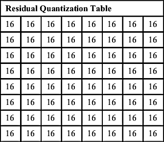
With P frames, a decision needs to be made for each macroblock, based on the motion estimation results. If the search for a match with another macroblock does not yield a good match in the previous I or P frame, then the macroblock must be coded as I frames are coded; that is, no temporal redundancy can be taken advantage of. If on the other hand, a good match is found in the previous I or P frame, then the current macroblock can be represented by a motion vector to the matching location in the previous frame, and by computing the residual, quantizing, and encoding (intercoded). The residual uses a uniform quantizer, and the DC component is treated just as the rest of the AC coefficients.
| Residual Quantization Table | |||||||
| 16 | 16 | 16 | 16 | 16 | 16 | 16 | 16 |
| 16 | 16 | 16 | 16 | 16 | 16 | 16 | 16 |
| 16 | 16 | 16 | 16 | 16 | 16 | 16 | 16 |
| 16 | 16 | 16 | 16 | 16 | 16 | 16 | 16 |
| 16 | 16 | 16 | 16 | 16 | 16 | 16 | 16 |
| 16 | 16 | 16 | 16 | 16 | 16 | 16 | 16 |
| 16 | 16 | 16 | 16 | 16 | 16 | 16 | 16 |
| 16 | 16 | 16 | 16 | 16 | 16 | 16 | 16 |
Some encoders also compare the number of bits used to encode the motion vector and residual, to ensure that there is a savings by using the predictive representation. Otherwise, the macroblock can be intracoded.
25.12. Compressing B Frames
B frames try to find a match using both preceding and following I or P frames for each macroblock. The encoder searches for a motion vector resulting in a good match over both the previous and following I or P frame and, if found, uses that frame to intercode the macroblock. If unsuccessful, than the macroblock must be intracoded. Another option is to use the motion vector but with both preceding and following frames simultaneously. When computing the residual, the B macroframe pixels are subtracted to the average of the macroblocks in the two I or P frames. This is done for each pixel, to compute the 256 residuals values, which are then quantized and encoded.
Many encoders then compare the number of bits used to encode the motion vector and residual using the preceding, following, or average of both to see which provides the most bit savings with predictive representation. Otherwise, the macroblock is intracoded.
25.13. Rate Control and Buffering
Video rate control an important part of image compression. The decoder has a video buffer of fixed size, and the encoding process must ensure that this buffer never underruns or overruns the buffer size, as either of these events can cause very noticeable discontinuities to the viewer.
The video compression and decompression process requires processing of the frames in a nonsequential order. Normally, this is done in “real-time”. Consider these three scenarios:
1. Video storage—Video frames arriving at 30 frames per minute must be compressed (encoded) and stored to a file.
2. Video readback—A compressed video file is decompressed (decoded), producing 30 video frames per minute
3. Streaming video—A video source at 30 frames per minute must be compressed (encoded) to transmit over a bandwidth limited channel (able to support maximum number of bits/second throughput), the decompressed (decoded) video is to be displayed at 30 frames per minute at the destination.
All of these scenarios will require buffering or temporary storage of video files during the encoding and decoding process. As mentioned above, this is due to the out-of-order processing of the video frames. The larger the GOP, containing longer sequences of I, P, and B frames, the more buffering is potentially needed.
The number of bits to encode a given frame depends on the video content, complexity and the type of video frame. A video frame with lots of constant background (the sky, a concrete wall) will take few bits to encode, whereas a complex static scene like a nature film will require much more bits. Fast moving, blurring scenes with a lot of camera panning will be somewhere in between as the quantizing of the high frequency DCT coefficients will tend to keep the number of bits moderate.
I frames take the most bits to represent, as there is no temporal redundancies to take advantage. Then comes P, and the fewest are B frames, since B frames can leverage motion vectors and predictions from both previous and following frames. P and B frames will require much less bits than I frames, if there is little temporal difference between successive frames, or conversely, may not be able to save any bits through motion estimation and vectors if the successive frames exhibit little temporal correlation.
Despite this, the average rate of the compressed video stream often needs to be held constant. The transmission channel carrying the compressed video signal may have a fixed bit rate, and keeping this bit rate low is the reason for compression in the first place. This does not mean the bits for each frame, say at a 30 Hz rate, will be equal, but that the average bit rate over a reasonable number of frames may need to be constant. This requires a buffer, to absorb higher numbers of bits from some frames, and provide enough bits to transmit for those frames encoded with few bits.
25.14. Quantization Scale Factor
Since the video content cannot be predicted in advance, and this content will cause variation amount of bits required to encode the video sequence, provision is made to dynamically force a reduction in the number of bits per frame. A scale factor is applied to the quantization process of the AC coefficients of the DCT, which is referred to as Mquant.
The AC coefficients are first multiplied by 8, then divided by the value in the quantization table, and then divided again by Mquant. Mquant can vary from 1 to 31, with a default value of 8. For the default level, Mquant just cancels the initial multiplication of 8.
One extreme is an Mquant of 1. In this case, all AC coefficients are multiplied by 8, then divided by the quantization table value. The results will tend to be larger, nonzero numbers, which will preserve more frequency information at the expense of using more bits to encode the slice. This results in higher quality frames.
The other extreme is an Mquant of 31. In this case, all AC coefficients are multiplied by 8, then divided by the quantization table value, then divided again by 31. The results will tend to be small, mostly zero numbers, which will remove most spatial frequency information and reduce bits to encode the slice. This results in lower quality frames. Mquant provides a means to trade quality verses compression rate, or number of bits to represent the video frame. Mquant is normally updated at the slice boundary and is sent to the decoder as part of the header information.
This process is complicated by the fact that human visual system is sensitive to video quality, especially for scenes with little temporal or motion activity. Preserving a reasonable consistent quality level needs to be considered as the Mquant scale factor is varied (Fig. 25.7).
Here the state of the decoder input buffer is shown. The buffer fills at a constant rate (positive slope) but empties discontinuously as various frame size I, P, and B data are read for each frame decoding process. The amount of data for each of these frames will vary according to video content and the quantization scale factors the encode process has chosen.
To ensure the encoder process never causes the decode buffer to overflow or underflow, it is modeled using a video buffer verifier (VBV) in the encoder. The input buffer in the decoder as conservatively sized, due to consumer cost sensitivity. The encoder will use the VBV model to mirror the actual video decoder state, and the state of the VBV can be used to drive the rate control algorithm, which in turn dynamically adjusts the quantization scale factor used in the encode process and sent to the decoder. This process closes the feedback loop in the encoder to ensure the decoder buffer does not over or under flow (Fig. 25.8).


The video encoder is shown in a simplified block diagram. The following steps take place in the video encoder:
1. Input video frames are buffered and then ordered. Each video frame is processed macroblock by macroblock.
2. For P or B frames, the video frame is compared to an encoded reference frame (another I or P frame). The motion estimation function searches and looks for matches between macroblocks of the current and previously encoded frames. The spatial offset between the macroblock position in the two frames is the motion vector associated with macroblock.
3. The motion vector points to be best matched macroblock in the previous frame, which is called a motion compensated prediction macroblock. It is subtracted from the current frame macroblock to form the residual or difference.
4. The difference is transformed using the DCT and quantized. The quantization also uses a scaling factor to regulate the average number of bits in compressed video frames.
5. The quantizer output, motion vector, and header information are entropy (variable length) coded, resulting in the compressed video bitstream.
6. In a feedback path, the quantized macroblocks are rescaled and transformed using the IDCT to generate the same difference or residual as the decoder. It has the same artifacts as the decoder due to the quantization processing, which is irreversible.
7. The quantized difference is added to the motion compensated prediction macroblock (see Step 2 above). This is used to form the reconstructed frame, which can be used as the reference frame for encoding the next frame. Recall the decoder will have access only to reconstructed video frames, not the actual original video frames, to use a reference frames (Fig. 25.9).
The video encoder is shown in a simplified block diagram. The following steps take place in the video encoder:
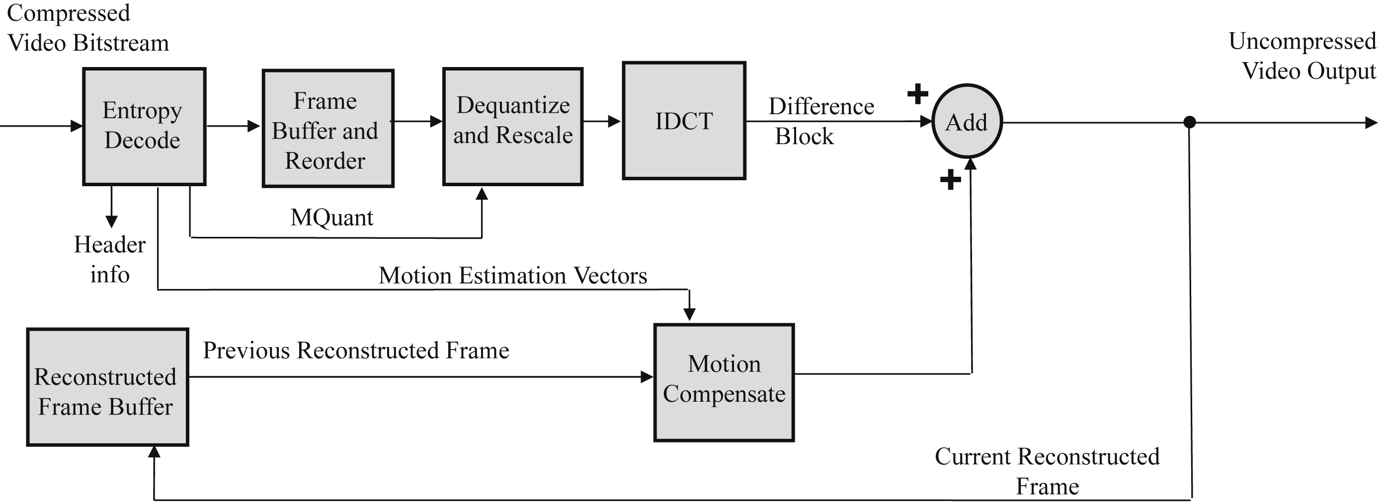
2. The data are ordered into video frames of different types (I, P,B), buffered and reordered.
3. For each frame, at the macroblock level, coefficients are rescaled and transformed using IDCT, to produce the difference or residual block.
4. The decoded motion vector is used to extract the macroblock data from a previous decoded video frame. This becomes the motion compensated prediction block for the current macroblock.
5. The difference block and the motion compensated prediction block are summed together to produce the reconstructed macroblock. Macroblock by macroblock, the video frame is reconstructed.
6. The reconstructed video frame is buffered and can be used to form prediction blocks for subsequent frames in the GOP. The buffered frames are output from the decoder in sequential order for viewing.
The decoder is basically a subset of the encoder functions, and it fortunately requires much less computations. This supports the often asymmetric nature of video compression. A video source can be compressed once, using higher performance broadcast equipment, and then distributed to many users, who can decode or decompress using much less costly consumer type equipment.
..................Content has been hidden....................
You can't read the all page of ebook, please click here login for view all page.