This chapter reviews the sampling of a signal and its conversion from the analog to the digital domain. Analog to digital converter measures the signal at rapid intervals is called samples, which outputs a digital signal proportional to the amplitude of an analog signal. The chapter throws light on sampling at low and high frequencies, the effects of revolution with time. Nyquist sampling rule is discussed in detail which leads to the elements of quantization. The effect of noise in increasing or decreasing the signal has also been discussed along with the concept of decibels. Decibel is a signal-to-power ratio and expressed logarithmically, which allows chains of circuits to process it. The two types of definition of dB have been discussed with power and amplitude emphasis which is of help to understand the differences in analog and digital signal processing.
Keywords
Digital signal processing; Nyquist; Quantization; Sampling effects; Signal to noise ratio
Now that we have the basic background material covered, let us start talking about digital signal processing (DSP). The starting point to understand is sampling and its affect on the signal of interest. To take an analog signal and convert it to a digital signal, we need to sample the signal using a device called an analog to digital converter (ADC). The ADC will measure the signal at rapid intervals, and these measurements are called samples. It will output a digital signal proportional to the amplitude of the analog signal at that instant. This can be compared to looking at an object with only a strobe light for illumination. You can see the object only when the strobe light flashes. If the object is not moving, then everything looks pretty much the same as if we used a normal, continuous light source. Where things get interesting is when we look at a moving object with the strobe light. If the object is moving rapidly, then the appearance of the motion can be quite different that when viewed under normal light. We can also see strange effects even if the object is moving fairly slowly, and we reduce the rate of the strobe light enough. Intuitively, we can see that what is important is the rate of the strobe light compared to the rate of movement of the illuminated object. As long as the light is strobing fast compared to the movement of the object, the movement of the object looks very fluid and normal. When the light is strobing slowly compared to the rate of object movement, the movement of the object looks funny, often like slow motion, as we can see the object is moving, but we miss the sense of continuous fluid movement.
Let us mention one more example many of us have experienced as a child. Imagine trying to make your own animated movie, and sketching a character on index cards. We want to depict this character moving, perhaps jumping and falling. We might sketch 20 or 40 cards, each showing the same character in sequential stages of this motion, with just small movement changes from one card to next. Once we are finished, we can show it to our friends by holding one edge of the deck of index cards, and flipping through it quickly by thumbing the other edge. We see our character in this continuous motion of jumping and falling by flipping through the deck of index cards in a second or two.
Actually, whenever we watch TV, this is what is occurring. But the TV is updating the screen at about 60 times per second, which is rapid enough that we do not notice the separate frames, and we think that we are seeing continuous motion.
So it makes sense that if we sample a signal very fast compared to how rapidly the signal is changing, we get a pretty accurate sampled representation of the signal, but if we sample too slow, we will see a distorted version of the signal.
3.1. Sampling Effects
Below are graphs of two different sinusoidal signals being sampled. The slower moving signal (lower frequency) in Fig. 3.1 can be represented accurately with the indicated sample rate, but the faster moving signal (higher frequency) in Fig. 3.2 is not accurately represented by our sample rate. In fact, it actually appears to be a slow moving (low frequency) signal, as indicated by the dashed line. This shows the importance of sampling “fast” enough for a given frequency signal.
Figure 3.1 Sampling a low-frequency signal (arrows indicate sample instants).
Figure 3.2 Sampling a high-frequency signal (same sample instants).
The dashed line shows how the sampled signal will appear if we connect the sample dots and smooth out the signal. Notice that since the actual (solid line) signal is changing so rapidly between sampling instants, this movement is not apparent in the sampled version of the signal. The sampled version actually appears to be a lower frequency signal than the actual signal. This effect is known as aliasing.
We need a way to quantify how fast we must sample to accurately represent a given signal. We also need to better understand exactly what is happening when aliasing occurs. It may seem strange, but there are some instances when aliasing can be useful.
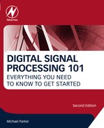
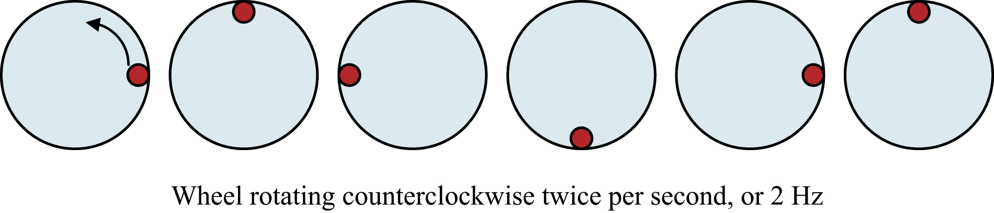
Let us go back to the analogy of the strobe light, and try another thought experiment. Imagine a spinning wheel, with a single dot near the edge. Let us set the strobe light to flash every 1/8 of a second, or 8 times per second. Below is shown what we see over six flashes, depending on how fast the wheel is rotating. Time increments from left to right in all figures (Figs. 3.3–3.10).
Figure 3.3 The dot moves 1/8 of a revolution, or π/4 radians with each strobe flash.
Figure 3.4 Now the dot moves twice as fast, ¼ of a revolution, or π/2 radians with each strobe flash.
Figure 3.5 The dot moves ½ of a revolution, or π radians with each strobe flash. It appears to alternate on each side of the circle with each flash. Can you be sure which direction the wheel is rotating?
Figure 3.6 The dot moves counterclockwise 3/4 of a revolution, or 3/2 π radians with each strobe flash. But it appears to be moving backward (clockwise).
Figure 3.7 The dot moves almost a complete revolution counterclockwise, 7/4 π radians with each strobe flash. Now it definitely appears to be moving backward (clockwise).
Figure 3.8 It looks like the dot stopped moving! What is happening is the dot completes exactly one revolution (2 π radians) every strobe interval. You can't tell whether the wheel is moving at all, spinning forwards or backwards. In fact, could the wheel be rotating twice per strobe interval (4 π radians)?
Figure 3.9 It sure looks the same as when the wheel was rotating once per second, or 1Hz. In fact, the wheel is moving 9/4 π radians with each strobe flash.
Figure 3.10 Now we stopped the wheel and started rotating backward at −π/4 radians with each strobe flash. Notice that this appears exactly the same as when we were rotating forward at 7/4 π radians with each strobe flash.
Does not all this look familiar from the previous chapter? The positive rotation is wrapping around and appears like a negative rotation as the wheel speed increases. And the rotation perception appears periodic in 2π radians per strobe, just like the angle measurements.
The reality is that once we sample a signal (this is what we are doing by flashing the strobe light), we cannot be sure what has happened in-between flashes. Our natural instinct is to assume that the signal (or dot in our example) took the shortest path from where it appears in one flash and then in the subsequent flash. But as we can see in the examples above, this can be misleading. The dot could be moving around the circle in the opposite direction (taking the longer path) to get to the point where we see it on the next flash. Or imagine that the circle is rotating in the assumed direction, but it rotates one full revolution plus “a little bit extra” every flash (Fig 3.9, or 9 Hz rate). What we see is only the “a little bit extra” on every flash. For that matter, it could go around 10 times plus the same “a little bit extra” and we could not tell the difference.
3.2. Nyquist Sampling Rule
To prevent all this, we have to come up with a sampling rule or convention. What we are going to agree is that we will always sample (or strobe) at least twice as fast as the frequency of the signal we are interested in. And in reality, we need to have some margin, so we better make sure we are sampling more than twice as fast as our signal. Going back to our example above, at what point do things start to get fishy?
Consider what happens when we start the wheel moving slowly in a counterclockwise direction. Everything looks fine until we reach a rotational speed of 4Hz. At this point the dot will appear to be alternating on either side of the circle with each strobe flash. Once we have reached this point, we can no longer tell which direction the wheel is rotating—it will look the same rotating both directions. This is the critical point, where we are sampling at exactly twice as fast as the signal. The sampling speed is the frequency of the strobe light (this would be analogous to the ADC sample frequency), eight times per second or 8Hz. The rotational speed of the wheel (our signal) is 4Hz.
If we spin the wheel any faster, it appears like it begins to move backward (clockwise), and by the time we reach a rotational speed of 8Hz, it appears to stop altogether. Spinning still faster will appear like the wheel moves forward again, until it again appears to start going backward again and the cycle repeats.
To summarize, whenever you have a sampled signal, you cannot really be sure of its frequency. But if you assume that the rule was followed—that the signal was sampled at more than twice the frequency of the signal, then the sampled signal will really represent the same frequency as the actual signal prior to sampling. The critical frequency which the signal must not ever exceed, which is one half of the sampling frequency, is called the Nyquist frequency.
If we follow this rule, then we can avoid the aliasing phenomenon we demonstrated with the moving wheel example above. Normally, what is done is that the ADC converter frequency is selected to be high enough to sample the signal in which we want to perform digital signal processing on. To make sure that unwanted signals above the Nyquist frequency do not enter the ADC and cause aliasing, the desired signal in usually passed through an analog low pass filter, which attenuates any unwanted high frequency content signals, just prior to the ADC.
A common example is the telephone system. Our voices are assumed to have a maximum frequency of about 3600Hz. At the microphone, our voice is filtered by an analog filter to eliminate, or at least substantially reduce, any frequencies above 3600Hz. Then the microphone signal is sampled at 8000Hz or 8kHz. All subsequent digital signal processing occurs on this 8kSPS (kilo-samples per second) signal. That is why if you hear music in the background while on the telephone, the music will sound flat or distorted. Our ears can detect up to about 15kHz frequencies, and music generally has frequency content exceeding 3600Hz. But little of this higher frequency content will be passed through the telephone system.
In the next chapter, we are going to start representing our signals and sampling in the frequency (or spectral) domain. What this means is that when we plot the signal spectrum, the X axis will represent increasing frequency (Fig. 3.11).
So far, we have covered the most important effects of sampling, but there remains one last issue related to sampling, which is quantization. We saw earlier how a digital signal is represented numerically, and how we must be sure that the numbers representing the sampled signal do not exceed the range of our binary or hexadecimal number range.
Figure 3.11 Nyquist frequency band.
3.3. Quantization
But what happens if the signals are very small? Remember in our discussion of signed fractional 8bit fixed point numbers, the range of values we could represent was from −1 to +1 (well, almost +1). The step size was 1/128, which works out to 0.0078125. Let us say the signal has an actual value of 0.5030 at the instant in time we sample it, using an 8bit ADC. How closely can the ADC represent this value? Let us compare this to a signal that is 1/10 the level of first sample or 0.0503. And again, consider a signal with value 1/10 the level as the second sample, at 0.00503. Below is a table showing the possible outputs from an 8bit ADC at each of these signal levels, and the error that will result in the conversion of the actual signal to sampled signal value. We say “possible outputs”, as we are assuming that the ADC will output either the value immediately above or below the actual input signal level (Table 3.1).
The actual error level remains more or less in the same range over the different signal ranges. This error level will fluctuate, depending upon the exact signal value, but with our 8bit signed example will always be less than 1/128, or 0.0087125. This fluctuating error signal will be seen as a form of noise or unwanted signal by the DSP. It is called quantization noise.
Table 3.1
8Bit Quantization Error
Signal Level
Closest 8Bit Representation
Hexadecimal Value
Actual Error
Error as a Percent of Signal Level (%)
0.50300
0.5000000
0x40
0.00300
0.596
0.50300
0.5078125
0x41
−0.0048128
0.957
0.05030
0.0468750
0x06
0.003425
6.809
0.05030
0.0546875
0x07
−0.0043875
8.722
0.00503
0.000000
0x00
0.00503
100
0.00503
0.0078125
0x01
−0.0027825
55.32
When the signal level is fairly large for the allowable range, (0.503 is close to one half the maximum value), the percentage error is small=less than 1%. As the signal level gets smaller, the error percentage gets larger, as the table shows.
What is happening is that the quantization noise is always present and is, on average, the same level (any noiselike signal will rise and fall randomly, so we usually concern ourselves with the average level). But as the input signal decreases in level, the quantization noise becomes more significant in a relative sense. Eventually, for very small input signal levels, the quantization noise can become so significant that it degrades the quality of whatever signal processing is to be performed. Think of it as like static on a car radio. As you get further from the radio station, the radio signal gets weaker, and eventually the static noise makes it difficult or unpleasant to listen to, even if you increase the volume.
So what can we do if our signal sometimes is strong (0.503 for example), and other times is weak (0.00503 for example)? Another way of saying this is that the signal has a large dynamic range. The dynamic range describes the ratio between the largest and smallest value of the signal, in this case 100.
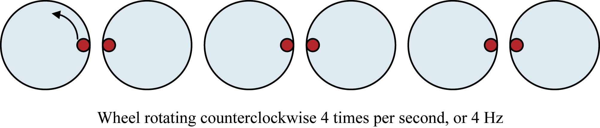
Suppose we exchange our 8bit ADC for a 16bit ADC? Then our maximum range is still from −1 to +1, but our step size is now 1/32,768, which works out to 0.000030518. Let us make a 16bit table similar to the 8bit example (Table 3.2).
What a difference! The actual error is always less than our step size, 1/32,768. But the error as a percent of signal level is dramatically improved. This is what we usually care about in signal processing. Because of the much smaller step size of the 16bit ADC, the quantization noise is much less, allowing even small signals to be represented with very good precision (<1%). Notice that even for our small signal level, 0.00503, the error about 0.1%.
Table 3.2
16Bit Quantization Error
Signal Level
Closest 16Bit Representation
Hexadecimal Value
Actual Error
Error as a Percent of Signal Level (%)
0.50300
0.5029907
0x4062
0.000009277
0.00185
0.50300
0.5030212
0x4063
−0.00002124
0.00422
0.05030
0.0502930
0x0670
0.00000703
0.0140
0.05030
0.0503235
0x0671
−0.0000235
0.0467
0.00503
0.005005
0xA4
0.0000251
0.499
0.00503
0.0050354
0xA5
−0.0000054
0.107
3.4. Signal to Noise Ratio
Another way of describing this is to introduce the concept of signal to noise power ratio (SNR). This describes the power of the largest signal compared to the background noise. This can be very easily seen on a frequency domain or spectral plot of a signal. There can be many sources of noise, but for now, we are only considering the quantization noise introduced by the ADC sampling.
SNR is usually expressed in decibels (denoted dB), using a logarithmic scale. The SNR of an ideal ADC can be determined by the following equation:
SNRquantization(dB)=6.02∗(Numberofbits)+1.76
Basically, for each additional bit of the ADC, 6dB of SNR is gained. An 8bit ADC is capable of representing a signal with an SNR of about 48dB, a 12bit ADC can do better at 72dB, and a 16bit will give up to 96dB. This only accounts for the effect of quantization noise; in practice there are other effects that also will degrade SNR in a system.
There is one last important point on decibels. These are very commonly used in many areas of digital signal processing subsystems. A decibel is simply a signal power ratio, similar to percentage. But because of the extremely high ratios commonly used (a billion is not uncommon), it is convenient to express this logarithmically. The logarithmic expression also allow chains of circuits or signal processing operations each with its own ratio (say of output power to input power) to simply be added up to find the final ratio.
Where people commonly get confused is in differentiating between signal levels or amplitude (voltage if an analog circuit) and signal power. Power measurements are virtual in the digital world, but can be directly measured in analog circuits in which DSP systems interface with.
The designations of “signal 1” and “signal 2” depends on the situation. For an RF power amplifier, the dB of gain will be the 10 log (output power/input power). For an ADC, the dB of SNR will be the 20 log (maximum input signal/quantization noise signal level). For a DAC, the dB of spurious free dynamic range will be 20 log (maximum output signal level/largest unwanted frequency component level generated by DAC circuits).
So dB can refer to many different ratios. But it is easy to get confused whether to use to multiplicative factor of 10 or 20, without understanding the reasoning behind this.
Voltage squared is proportional to power. If a given voltage is doubled in a circuit, it requires four times as much power. This goes back to a basic Ohm's law equation.
Power=Voltage2/Resistance
In many analog circuits, signal power is used, because that is what the lab instruments work with, and while different systems may use different resistance levels, power is universal (however, 50Ω is the most common standard in most analog systems).
The important point is that since voltage is squared, this effect needs to be taken into account in the computation of logarithmic decibel relation. Remember, log xy=y log x. Hence, the multiply factor of “2” is required for voltage ratios, changing the “10” to a “20”.
In the digital world, the concept of resistance and power do not exist. A given signal has specific amplitude, expressed in a digital numerical system (such as signed fractional or integer for example).
Understanding dB increases using the two measurement methods is important. Let us look at doubling of the amplitude ratio and doubling of the power ratio.
6.02dBvoltage=6.02dBdigitalvalue=20⋅log(2/1)
3.01dBpower=10⋅log(2/1)
This is why shifting a digital signal left 1bit (multiply by 2) will cause a 6dB signal power increase, and why so often the term 6dB/bit is used in conjunction with ADCs, DACs, or digital systems in general.
By the same reasoning, doubling in power to an RF engineer means a 3dB increase. This will also impact the entire system. Coding gain, as used with error correcting code methods, is based upon power. All signals at antenna interfaces are defined in terms of power, and the decibels used will be power ratios.
In both systems, ratios of equal power or voltage are 0dB. For example, a unity gain amplifier has again of 0dB.
0dBpower=10⋅log(1/1)
A loss would be expressed as a negative dB. For example, a circuit whose output is equal to ½ the input power.