Chapter 20
Automotive Radar∗
Abstract
Radar is becoming an important automotive technology. Automotive radar systems are the primary sensor used in adaptive cruise control and are a critical sensor system in autonomous driving assistance systems (ADAS). In ADAS, automotive radar is one of the several sensor systems for collision avoidance, pedestrian and cyclist detection, and complements vision-based camera-sensing systems. The radar technology generally used is frequency-modulated continuous-wave or FMCW radar, which is quite different from the pulse-Doppler radar. The analog and RF hardware in millimeter FMCW is much less costly than that of pulse-Doppler radar. In addition, the digital processing requirements are generally modest and can be performed in low-cost field programmable gate arrays, microprocessors with specialized acceleration engines, or specialized application-specific integrated circuits.
Keywords
Angle of arrival; CA-CFAR; Constant false alarm rate; FMCW doppler processing; FMCW radar; FMCW range processing; OS-CFAR
Radar is becoming an important automotive technology. Automotive radar systems are the primary sensor used in adaptive cruise control and are a critical sensor system in autonomous driving assistance systems (ADAS). In ADAS, automotive radar is one of the several sensor systems for collision avoidance, pedestrian and cyclist detection, and complements vision-based camera-sensing systems. The radar technology generally used is frequency-modulated continuous-wave or FMCW radar, which is quite different than the pulse-Doppler radar. The analog and RF hardware in FMCW is considerably less complex than that of pulse-Doppler radar. In addition, the digital processing requirements are generally modest and can be performed in low-cost field programmable gate arrays, microprocessors with specialized acceleration engines, or specialized application-specific integrated circuits.
Pulse-Doppler radars are used in longer range radars where the range can be one kilometer to hundreds of kilometers. The transmitter operates for a short duration, then the system switches to receive mode until the next transmit pulse. The pulse-Doppler radar sends successive pulses at specific intervals or a pulse repetition interval. As the radar returns, the reflections are processed coherently to extract range and relative motion of detected objects. Sophisticated processing methods are employed to further process radar returns and extract target data even when heavily obscured by ground clutter or background returns surrounding the object(s) of interest. However, with automotive radar, the range can be as short as a few meters to as much as a few hundred meters. For a range of 2 m, the round-trip transit time of the radar pulse is 13 ns. This short range requires that the transmitter and receiver operate simultaneously, which requires separate antennas. The pulse-Doppler radar sends a pulse periodically, and the ratio of the time the transmitter is active to the total time elapsed is the duty cycle. Since duty cycles are typically small, this ratio limits the total transmit power. The power, in turn limits the range of detection. Achieving a 1- to 2-m range resolution also requires very high-speed analog pulsing circuitry, high digital sample rates, high digital signal processing capability, which is not feasible in low cost automotive systems.
20.1. Frequency-Modulated Continuous-Wave Theory
FMCW radar is a much more optimal method for short range radar. FMCW does not sent out pulses and then monitor the returns or radar echo. Rather, a carrier frequency transmits continuously. To extract useful information from the continuous return echo, the carrier frequency is increased steadily over time, and then decreased, as shown in Fig. 20.1. Both the transmitter and receiver operate continuously. To prevent the transmit signal from leaking into the receiver, separate transmit and receive antennas are used.

20.2. Frequency-Modulated Continuous-Wave Range Detection
The radar must determine the range of objects detected. In FMCW, the range is accomplished by measuring the instantaneous receive frequency difference, or delta, from the transmit frequency. During the positive frequency ramp portion of the transmit cycle, the receive frequency will be somewhat less than the transmit frequency, depending on the time delay. During the negative frequency ramp portion of the transmit cycle, the receive frequency will be greater than the transmit frequency, again depending on the time delay. These frequency differences, or offsets, will be proportional to the round-trip delay time, which provides a means to measure the range. The greater the range, the more time delay there is from the transmitter to the receiver. Since the transmit frequency is constantly changing, the difference between transmit and receive frequencies at any given instant will be proportional to the elapsed time for the transmit signal to travel from the radar to the target and back.
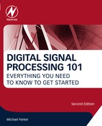
An example block diagram of an FMCW radar is shown in Fig. 20.2. Automotive radars operate in the millimeter range, meaning the wavelength of the transmit signal is a few millimeters. Common frequencies used are 24 GHz (λ = 12.5 mm) and 77 GHz (λ = 3.9 mm). Millimeter wave frequencies are used because of the small antenna size needed, relative availability of spectrum, and rapid attenuation of radio signals (automotive radar ranges are limited to hundreds of meters). By using FMCW, there is no amplitude modulation, and the transmitter only varies in frequency. Use of FM allows for the transmit circuit to operate in saturation, which is the most efficient mode for any RF amplifier.
Due to the analog mixer circuit, the receive low-pass filter only needs to pass the difference between the receive and transmit signals. It does not need to pass the 500 MHz bandwidth of the receive signal over the transmit cycle. This passing of the difference in signals is most easily illustrated by example. Assuming receive reflections at the minimum and maximum ranges of distances 1 and 300 m.
With a frequency ramp of 500 MHz in 0.5 ms, or 1 kHz per ns, the frequency of the receive signal will be as follows, using the speed of light at 3 × 10⁸ m/s:
During the positive frequency ramp, the return from the object at a 1 m distance will be a −7 kHz offset. During the negative frequency ramp, the return from the object at a 1 m distance will be a +7 kHz offset.
During the positive frequency ramp, the return from the object at a 300 m distance will be a −2 MHz offset. During the negative frequency ramp, the return from the object at a 1 m distance will be +2 MHz offset.
These offsets indicate that the receiver input will have frequencies in the range of +/−2 MHz, depending on the range of the target generating the return. This frequency can be detected by operating a fast Fourier transform (FFT) for the time intervals shown in Fig. 20.3. If the receiver samples at 5 MSPS (mega samples per second), then for a receiver FFT sampling interval of about 0.4 ms, a 2048-point FFT can be used, which will give a frequency resolution of 1 kHz, sufficient for a fraction-of-a-meter-range resolution. Further resolution is possible by performing an interpolation of the FFT output.

This observed frequency offset provides the receiver range returns but cannot be used to discriminate between oncoming traffic, traffic traveling in same direction, or stationary objects at similar ranges. To make this discrimination, the Doppler frequency shift of the return must be exploited.
20.3. Frequency-Modulated Continuous-Wave Doppler Detection
A simple example can illustrate how the Doppler frequency shift can be detected. Assume the 77 GHz radar-equipped automobile is traveling at 80 km/h, or 22.2 m/s, and consider three targets at 30 m distance—one an oncoming auto at 50 km/h, another traveling in same direction at 100 km/h, and a stationary object. When the objects are closing range, the Doppler frequency shift will be positive, meaning the return signal will have a higher frequency than that transmitted. Intuitively, this behavior is due to the wave crests of the signal appearing closer together due to the closing range. Conversely, when the range between the radar and the target is opening, or getting larger, the result will be a negative Doppler frequency shift. The amount of Doppler shift can be calculated as shown in Eq. (20.1).
 (20.1)
These Doppler shifts will offset the detected frequency differences on both the positive and negative frequency ramps. When there is no relative motion, and no Doppler shift, the difference in the receive frequency will be equal, but of opposite sign, in the positive and negative frequency ramps. So the Doppler shift can be found by comparing the receive frequency offsets during the positive and negative portions of the frequency ramp of the transmit signal. The relationship is described in Eq. (20.2), where the range and the relative velocity can be determined by the output of the FFT using the results during both positive and negative frequency ramps of the transmitter.
The frequencies seen by the receiver and processed by the FFT are shown in Fig. 20.4. The receiver is demodulated, or down converted, by using the transmit signal as the local oscillator (LO), so the FFT will process the frequency difference between the transmit and receive waveforms. Fig. 20.4 shows only one target pulse return; however, there could be multiple (three in our example) different targets generating multiple frequencies for the FFT to detect.
Returning to the example, there are three targets at 30 m distance—an oncoming automobile at 50 km/h, another traveling in same direction at 100 km/h, and a stationary object. The automobile mounting the radar is traveling at 80 km/h, or 22.2 m/s. For all three targets at 30 m, the receive frequency offset will be as follows:
Frequency offset: +/−200 kHz on the negative and positive frequency ramp, respectively.
The Doppler offset must be added to the frequency offset caused by the range delay. The values are summarized in Table 20.1.
Table 20.1
Target Frequency Offsets Due to Range and Doppler
| 30 m Range, 80 km/h Radar Vehicle Speed | Negative Ramp Frequency Offset Due to 30 m Range | Positive Ramp Frequency Offset Due to 30 m Range | Frequency Offset Due to Doppler (Negative and Positive Ramp) | Total Observed Negative/Positive Frequency Offset |
| Oncoming at 50 km/hr | 200 kHz | −200 kHz | 18.5 KH | 218.5 kHz/−181.5 kHz |
| Stationary object | 200 kHz | −200 kHz | 11.4 kHz | 211.4 kHz/−188.6 kHz |
| Same direction at 100 km/h | 200 kHz | −200 kHz | −2.8 KHz | 197.2 kHz/−202.8 kHz |

Using only the observed negative and positive frequency offsets, both the range and relative Doppler shift of the targets can be determined using Eqs. 20.3–20.5. Since the forward velocity of the radar-equipped auto is known, the velocities of the targets can be easily computed. Similarly, the frequency ramp rate of the radar is also a known quantity.
The frequency ramp rate in this case is 500 MHz over 0.5 ms, or rate of 1000 GHz per second. Plugging in our example values, we find:
For vehicle approaching 50 km/h:
The other target calculations are similar.
However, real-world systems often have many targets, some of which are of interest and some of which are not. Along with clutter, it may not be possible to pair up many frequencies in the negative and positive ramp period. This problem is known as ambiguities in radar jargon. One approach to the problem is varying the duration and frequency of the ramps and evaluating how the detected frequencies move in the spectrum with different steepness of frequency ramps.
More commonly, the range and velocity detection processing is performed separately, using multiple sample intervals. This is a combination of pulse-Doppler and FMCW techniques. Essentially, it is a pulsed system that utilizes FMCW modulation. But first a quick review of the FMCW RF and antennas.
20.4. Frequency-Modulated Continuous-Wave Radar Link Budget
Radar performance is governed by the link budget equations, which determine what level of receive signal are available for detection. A simplified version of the radar link budget is expressed in Eq. (20.6).
where: Ptrx is the peak transmit power; G is the transmit and receive antenna gain; σ is the radar cross section or area of the target; λ is the radar wavelength; τ is the duty cycle of transmitter; R is the range to the target.
Often, parameters are specified on a logarithmic scale, using decibels (dB), or dBm (dB referenced to 1 mW). This scale will be used in this case, but figures in Watts will also be given. We must make a few assumptions. With an achievable receiver noise figure of 5 dB, the receiver sensitivity should be about −120 dBm (10−15 W). Assuming about 20 dB signal-to-noise ratio to achieve reasonable frequency detection, results in a requirement that Prcv should be at least 100 dBm (10−13 W) under worst-case circumstances.
We will use an antenna gain of 30 dB, or 1000. For a parabolic antenna, the gain in the direction of the bore sight of the antenna can be calculated as shown in Eq. (20.7).
Working backward, we find the area required for the antenna at 77 GHz is 0.0012 m2, which works out to a diameter of 0.04 m, or 4 cm, which is a very reasonable size to mount on the front of a vehicle. (Note, we need at least one transmit and one receiver antenna.)
The duty cycle τ in FMCW is 100%, or 1. If we assume a transmit power of 0.1 W (20 dBm), a maximum range of 300 m, and a target vehicle reflecting area of 1 m2, we can find the worst-case receive power under reasonable circumstances.
Using a very close range, say 2 m, and same cross-sectional area of 10 m2 (the back of a tractor trailer), we can calculate the maximum Prcv we can expect under reasonable circumstances.
These calculations tell us that our system requires a very high-dynamic–range receiver, on the order of 120 dB. The high-dynamic range imposes a severe requirement on linearity of the receiver and the analog-to-digital converter (ADC). However, a large target only 2 m away will obscure the radar line of sight for other targets. Therefore, an analog automatic gain control (AGC) loop can be used to reduce the dynamic range of the receiver and ADC by desensitizing the receiver with attenuation in the presence of extremely large returns.
Full sensitivity could be desired in a slightly less demanding situation, such as a 1 m2 target at 4 m distance, and still used to detect other targets at much longer range. In this case, the large return will have a receive power:
The use of AGC reduces the dynamic range requirement to about 95 dBm, achievable using a 16-bit ADC. To give some margin, the ADC could be operated with 32X oversampling (beyond Nyquist requirements) to achieve another effective 3 bits, or reducing the quantization noise floor a further 18 dB. Alternatively, an 18-bit ADC could be used, but would likely be much more costly.
20.5. Frequency-Modulated Continuous-Wave Implementation Considerations
On the analog side, the transmitter can be implemented using a direct digital synthesizer (DDS) with a standard reference crystal. The DDS generates an analog frequency ramp reference for the phase-locked loop (PLL) to generate the desired transmit frequency modulation. For example, if the PLL has a divider of 1000, then in our example, the reference would be centered at 77 MHz, with a 5 MHz frequency ramp. This analog ramp signal drives the reference of a PLL, which disciplines a 77 GHz oscillator. The oscillator output of the circuit is amplified and produces the continuous-wave signal ramping up and down over 500 MHz with a center frequency of 77 GHz. Filtering and matching circuits at 77 GHz can be accomplished using passive components etched into high-epsilon R dielectric circuit cards, minimizing the components required. Fig. 20.5 illustrates an analog circuit block diagram.
In the receiver, the front end requires filtering and a low-noise amplifier (LNA), followed by a quadrature demodulator. The quadrature demodulator mixes the 77 GHz receive signal with the ramping transmit signal, outputting a complex baseband signal that contains the difference between the transit and receive waveforms at any given instant. The ramping has been canceled out, as we see fixed frequencies depending on the range and Doppler shift of the target returns. Again, the high-frequency filtering at 77 GHz can be implemented using etched passive components. The output of the quadrature demodulator will be at low frequency, up to +/− 2 MHz at maximum range. Therefore, traditional passive components and operational amplifiers can be used to provide antialiasing low-pass filtering prior to the in-phase (I) and quadrature (Q) ADCs. Alternately, an intermediate frequency architecture could be used, but would require an offset receive LO generation circuit.

20.6. Frequency-Modulated Continuous-Wave Interference
Eventually, there may be many vehicles equipped with radars operating at 77 or 24 GHz. The radar transmitter of an oncoming vehicle will likely produce a much stronger signal than most target reflections. However, the transmitter is operating over hundreds of MHz, specifically 500 MHz in this example. The receiver input bandwidth is on the order of 5 MHz, or about 1% of transmit bandwidth. Interference can only occur if the oncoming transmitter is sweeping through this 1% of its bandwidth at the same time the other receiver happens to also be sweeping through that particular bandwidth. Statistically, this overlap is not likely to occur very often, and when it does, it can be eliminated by randomly adjusting the transmit ramp timing. This problem is common in systems where many devices infrequently communicate over a shared channel using random access techniques.
20.7. Frequency-Modulated Continuous-Wave Beamforming
The radar system described so far can detect range and velocity or targets, but cannot provide any information on the direction of the target, other than it is in front of the vehicle, within the beam width of the antenna. Directivity can be determined if the system has the ability to sweep or steer the radar transmit or receive antenna directivity and monitor the variations in target return echo across the sweep.
The described system is assumed to use parabolic antennas. The parabolic antenna focuses the transmitted or received electromagnetic wave in a specific direction. The degree of focusing depends primarily on the antenna area and wavelength. Using millimeter wave radar allows for small antennas.
A parabolic antenna can be “aimed” by mechanically orientating it in the desired direction, which is limited by the speed of mechanical movement, as well as reliability and cost issues. Instead, electronic beam steering is used. The antenna becomes either a linear or rectangular array of separate receive or transmit antennas. By coherently combining the separate antenna signals, the effects of constructive and destructive wave front combining will result in maximum gain in a specific direction, and minimum gain on other directions.
In the automotive radar case, elevation steering (up and down) of the radar is generally not required, so a two-dimensional antenna array is not required. A linear array, or line of antennas, will permit azimuth (side to side) steering of the antenna. The trade-off is cost and complexity. In this case, steering of the receive direction is more straightforward, due to the digital processing of the receive signal. Each receiver must individually vary the phase of receive signal.
This phase adjustment provides for steerable directivity of the antenna beam. Only when the receive signal arrives in-phase across all the antenna elements will the maximum signal strength occur. The array antenna provides the ability to “aim” the main lobe of the antenna in a desired direction. Each antenna element must have a delay, or phase adjustment, such that after this adjustment, all elements will have a common phase of the signal. If the angle θ = 0, then all the elements will receive the signal simultaneously, and no phase adjustment is necessary. At a nonzero angle, each element will have a delay to provide alignment of the wave front across the antenna array, as shown in Fig. 20.6.

The electronic steerable antenna requires replicating the analog receiver circuits for each of the N antenna receive nodes. Fortunately for millimeter radars, much of the circuitry, including antenna patches, filters, and matching circuits can be implemented directly on the printed circuit board. The LNA, quadrature demodulators, and ADCs must also be replicated for each of the N nodes.
Digitally, each set of I and Q inputs from the ADC pair of each antenna node must be delayed in-phase. This delay is accomplished by a complex multiplier with N separate complex coefficients Wi for each of the N receive nodes. The control processor “sweeps” the receive antenna by updating N complex coefficients periodically and monitoring the changes in target-return amplitudes.
In a forward-looking automotive radar, the degree of desired azimuth steering may only be 5–10 degrees off the automobile centerline. In terms of cost effectiveness, it may be possible to use a parabolic transmit antenna with sufficient antenna lobe beam width and utilize a narrower lobe beam steering receive antenna to provide the ability to distinguish targets across different azimuths. Alternately, a more complex transmitter and transmit beamforming antenna can also be used to provide more gain in the desired transmit azimuth direction, but at greater cost and complexity.
20.8. Frequency-Modulated Continuous-Wave Range-Doppler Processing
Returning to the signal processing, the method combining pulse-Doppler and FMCW modulation is described. This includes multiple receive antennas, range FFT processing, Doppler FFT processing, noncoherent magnitude detection, constant false alarm rate (CFAR) processing, even angle of arrival (AoA) estimation (Fig. 20.7). Much of this processing can be performed in parallel, with hardware-based architecture (FPGA or ASIC).
Automotive radar systems require low latency processing. To meet latency requirements, much of the processing needs to be performed in parallel. For example, a typical radar frame time is 40 ms, meaning that the entire radar processing must be completed and results generated in that time, at a rate 25 times per second. The signal processing would need to be performed in significantly less time, to allow for subsequent host CPU processing to organize and sort the detection results. In addition, memory access times must be considered, as the amount of data being processed requires storage of intermediate results, for the radar “corner turn” and to store the radar “data cube,” which is generated during each frame.

Several system key parameters will determine the FMCW radar capability and are needed to size the signal processing and memory capabilities. For the purposes of discussion, the following will be assumed:
• 40 m, frame time, with 25 ms for sampling and signal processing,
• Eight receive antennas,
• 20 MSPS sample rate per ADC,
• 1024 samples per pulse (real data),
• 256 pulses per frame, and
• 800 MBps or greater external SRAM memory access rate.
20.9. Frequency-Modulated Continuous-Wave Radar Front-End Processing
Radar front-end processing includes the following steps:
• Sample the data during the each pulse across all antennas—requires buffering 1024 samples per ADC input (or per antenna) k,
• Apply window function to each block of date from each antenna;
• Performing range 1024 FFT across the pulse interval;
• Storing range FFT data to external memory;
• After all pulses have been processed and stored to external memory, read out data (“corner turn”), apply window function;
• Perform Doppler FFT processing; and
• Save each Doppler FFT output data to external memory, overwriting Doppler input data.
The FFT engine is a block-based FFT, processing each antenna data in turn, which necessitates storage buffer to capture the 1024 samples from each ADC during the pulse interval. Note that the ADC data is real data (complex portion equals zero), since FM input signal is a real signal, not complex. Therefore, the FFT produces a 1024 sample complex symmetric output. Due to the symmetry of the FFT output, only 512 complex samples need to be saved, as the other 512 complex samples are redundant and discarded.
A timing diagram illustrates the parallelism of the processing (Fig. 20.8). The range of FFT processing time is determined by the sampling rate. The range active sampling time is 50 ns (at 20 MSPS) × 1024 real samples, which gives 51.2 μs. There is a small interval between pulse intervals, set here at 5 μs. This provides enough time for all receive radar returns to arrive, so will not overlap in the next pulse interval. The total sampling time is therefore (51.2 μs + 5 μs) × 256 (the number of pulses), which is about 14.4 ms.

During this 51.2 μs pulse interval time, the transmitter is operating with a linear ramping FM waveform. The transmit and receive frequencies are mixed, and this mixer output, or frequency difference, is what is sampled by the ADC. Since the transmit frequency ramp is only positive during the pulse interval, only a real frequency difference is sampled. Therefore, quadrature sampling (used for complex baseband signals) is not required.
After the range sampling time of 14.4 ms the back-end processing including Doppler, complex magnitude, CFAR, and AoA estimation is estimated to take about 10.5 ms. These functions can be largely done with parallel processing capabilities to allow for a substantial reduction in processing time for these complex functions and allows the remaining 15 ms for host processing of the output data (assuming a 40 ms period).
A single FFT can process all eight antenna range data. Each antenna data is double buffered to allow for flexible, nonsynchronous clocking of ADCs. Assuming the FFT can process one input sample per clock cycle and is operating at 200 MHz. Therefore, one FFT can keep up with the aggregate input sample rate of eight times 20 or 160 MSPS. The FFT processes each block of 1024 antenna samples. This will repeat across all eight antennas, creating the data structure on the lower left of Fig. 20.9. The FFT output data results will be written to the external memory, interleaving the data between eight antennas. This whole process repeats 256 times, which is the number of transmitter pulses and creates the radar data cube of post-FFT range data shown in the middle of Fig. 20.9.

The FFT processing and memory writes occur in parallel with the receive data sampling, so at the end of the 14.4 ms, the range data cube is contained in the external memory. This memory also requires access in bursts of consecutive 8 bytes (or 9 bit bytes), which is four complex samples. The sequential burst access requirement must be observed to maintain maximum memory bandwidth, and the data ordering must be considered for Doppler and CFAR processing.
The FFT processing and memory writes occur in parallel with the receive data sampling, so at the end of the 14.4 ms, the range data cube is contained in the external memory. The memory size is 8 (number of antennas) × 512 (number of range FFT samples) × 256 (number of pulses) × 2 (complex data) × 2 (16 or 18 bit data), which requires a 4 MB memory. Often a burst size must be observed, and also sequential burst access memory requirements needed to maintain maximum memory bandwidth and the data ordering for subsequent Doppler and CFAR processing.
20.10. Frequency-Modulated Continuous-Wave Pulse-Doppler Processing
The radar data cube now need to be read back into the FPGA for Doppler processing. Recall in the FMCW radar, it is possible to perform both range and Doppler estimation by using triangular frequency pulses, with both positive and negative frequency ramps. This technique may be suitable for simple detection, with few targets, such as blind spot detection. However, in a forward-looking radar, there will be myriad of targets, and this more sophisticated processing is needed.
The Doppler FFT will be performed for each range bin, across a specific range for all 256 pulses. This requires a total of 512 FFTs (as there are 512 range bins) to be processed for each antenna, each of length 256. A single FFT engine will perform the 8 × 512 FFTs, requiring 8 × 512 × 256 clock cycles at 200 MHz, or 5.25 ms. The limitation is the memory bandwidth, as the Doppler FFT data must be both read in from the external memory, and then written back out, overlaying the original 256 block of complex samples. A 5 ns per 4-byte memory transaction, this requires 10.5 ms in total.
A single FFT engine can perform both range and Doppler FFTs, as these happen at different times. During the range FFT processing phase, the FFT operates as a 1024-point FFT. In Doppler processing, the same FFT operates at 256 points. If different combinations of range and Doppler sizes are needed, the FFT can be dynamically configured for the appropriate 2N size transform.
The indexing of the memory is important in the organization of the radar dataflow. In pulse-Doppler radars, the range data is normally written into an external memory in sequential order with regard to the range samples. Each radar pulse range data is written in blocks, one block after the other. For Doppler processing, the data must be read in a different order. This reordering is known as the corner turn in radar terminology, and in DDR memories, internal buffering is needed to manage this with consideration of the burst length access requirements.
The data must be read from the memory for Doppler FFT processing (Fig. 20.10). Due to the CFAR processing requirements in the back end, the antenna data interleaved in the external memory. However, the burst data reads for the Doppler processing are in a different order than the postrange FFT writes. While the antenna data is still interleaved in the burst accesses, the burst addresses now index along the 256 long pulse counts, rather than the 512 long range counts. Each block of 256 complex samples is read in for a specific range, across the 256 pulses. Eight of the FFT data blocks are buffered, as the antenna data must be deinterleaved as it is read from the external memory.
The Doppler FFT processing will replace the individual range bin data for each pulse interval with a frequency distribution for individual range bin, allowing determination of radial velocity. At this point, target detections can be made on the basis of range and relative velocity to the radar system. This has been performed for each of the eight antenna receive inputs.
A plot of range-Doppler data is depicted (Fig. 20.11).
In Fig. 20.10, the first three of the memory accesses have been discussed. The fourth access occurs during AoA estimation, which will be covered shortly. An internal data transfer also occurs, whereas the Doppler FFT results are processed real time as they are generated by the detection process, which operates largely in parallel.


20.11. Frequency-Modulated Continuous-Wave Radar Back-End Processing
The back-end processing is focused on detection. Due to the stochastic nature and often high levels of noise and clutter, detection is far from simple. Most radar systems use some sort of CFAR detection algorithm to determine whether it is a legitimate target. This involves comparing the magnitude, or magnitude squared of a given range and Doppler cell to an estimate of the clutter and noise in nearby cells. When this ratio exceeds a given threshold, then detection is assumed. By using a variable and local estimate of clutter, the rate of false alarms should, in theory, remain at a constant level.
20.12. Noncoherent Antenna Magnitude Summation
For the CFAR detection process, the input energy from all antennas must be used. To facilitate this, the outputs of the eight FFTs for a give range and Doppler are combined, across the eight antennas, using the equation below.

This noncoherent combining results in an array of magnitude squared data for each range and Doppler point. It essentially collapses the 3-D radar data cube into a 2-D array, by combining the individual antenna data (Fig. 20.12). In this case, the 2-D array will be 512 × 256, representing the detected energy at each range-Doppler combination. Since this is noncoherent, the value is real, not complex, which also reduces the data storage requirements by one half. A given location is often referred to as a “cell.” Note this collapsing is done within the FPGA, and the 3-D radar data cube data is still preserved in the external memory for later use in AoA estimation.
The front processing across for the eight antennas is processed in an interleaved manner. Therefore, the output of the Doppler data is processed as it is generated. Due to the organization in the external memory, all eight antennas data for a given range and Doppler value can be accessed at the same time it is written into the external memory.
Two basic variations of CFAR detection are commonly used. Cell averaging, or CA-CFAR, performs an average calculation of the magnitude (or magnitude squared) of the cells surrounding the cell under test (CUT). Since every cell in the range-Doppler array must be tested, this results in a sliding window-type calculation. The other basic type of CFAR is ordered statistic, or OS-CFAR. In this case, magnitude (or magnitude squared) of the cells surrounding the CUT are ranked, and a median, or kth order value is used as the clutter estimate. OS-CFAR can be more difficult to process, but it has proven in many scenarios to provide a superior clutter estimate, and less sensitivity to regions of strong clutter obscuring target detection.
The front-end processing generates the range-Doppler array at a rate of one cell every 100 ns, or at a 10 MSPS rate. Therefore, the detection processing must be able to operate at the same rate.

20.13. Cell Averaging–Constant False Alarm Rate
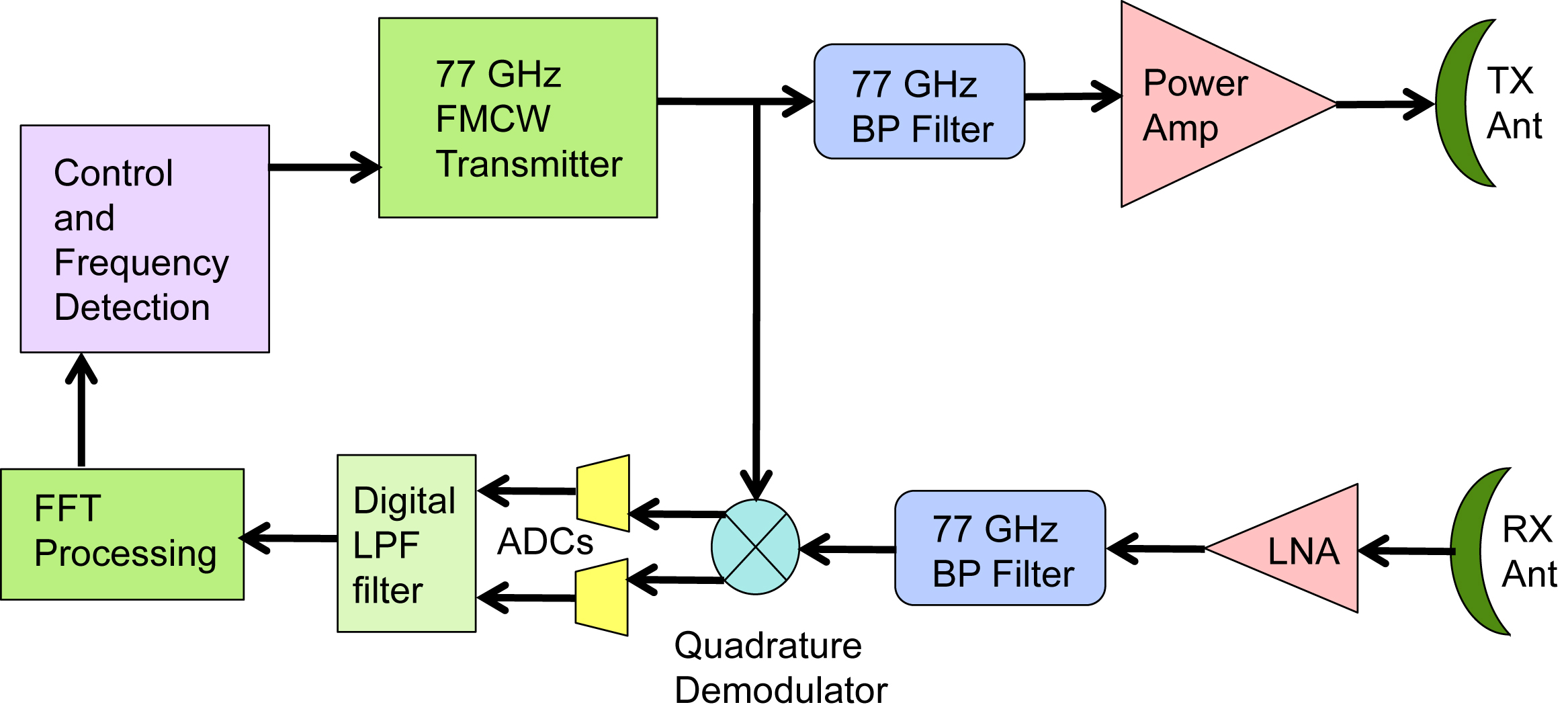
As each set of 256 Doppler row data is generated, it can be stored in a single block memory. For an N × N CFAR window, N + 4 rows need to be stored. As the CUT moves through the array, the next row of data can overwrite the oldest row. This process is depicted in Fig. 20.13, where the 7 × 7 block of cells is the sliding window. The upper cells are the stored row data, and lower cells are in the process of being computed and written into the array for CFAR processing.
A variation of CA-CFAR is to use weighted averaging, rather than simple averaging. Using multipliers, the cells can be weight the cells in the sliding window by coefficients stored in local memories. This allows for a “tapering” of the cell values near the sliding window boundaries, rather than a sharp cutoff. Weighting can also be used to deemphasize the guard cells immediately adjacent to the CUT, to avoid including possible target energy in the clutter estimate (left side of Fig. 20.14). The coefficient can also be modified near the array boundaries; for example, doubling the weighting on one side when the cells on the other side of CUT do not exist. Other options would be to perhaps expand the guard cells in regions of high Doppler, when there tends to be more spreading of target return energy across multiple cells.
Filtering or weighting can also better concentrate CUT energy from immediately adjacent cells. This would be to provide better CUT estimates when the target energy is split across two or more cells (Fig. 20.14).
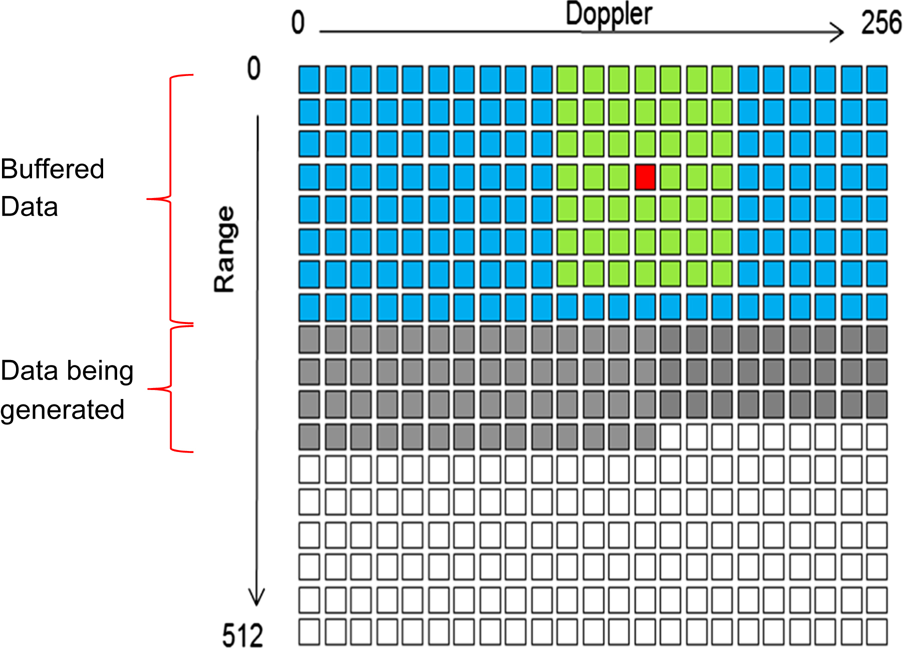
Multiple sliding windows can be used to expand the regions used to estimate clutter. In this case, two regions, one leading and one lagging the CUT, are used, with the results averaged to provide the final clutter interference estimate. This could be computed at the same rate but requires more computational resources (Fig. 20.15).

20.14. Ordered Sort–Constant False Alarm Rate
The other popular CFAR algorithm is ordered sort (OS). This is more a logic intensive algorithm, as it requires sorting. As the N × N window moves across the array, N new magnitude2 samples are introduced to the sliding window, and N old samples. As mentioned above, new samples are generated every 100 ns, or at a 10 MSPS rate.
Each new sample requires a new sort of all the elements in the window. This can be accomplished for N elements, which must take place in a single clock cycle. Here a window size of 7 × 7 is shown. The 49 element window size resorted seven times for the seven new samples as the window is shifted to a new CUT location. The window slides every 100 ns, so provides 10 clock cycles on average, as shown for OS-CFAR in Fig. 20.16. To maximize sort efficiency, the OS-CFAR window slides to right one sample at a time across Doppler index, then drops to next row and cycles in the opposite direction repeating until 2-D array is completed.
To build an efficient single clock cycle–sort algorithm, it is necessary to add only one new element per sort, while discarding the oldest element. When the CUT increments to a new row, a complete new window will be started, with all new cells, necessitating many clock cycles to complete the sort. A revised method for selecting the next CUT and therefore direction of sliding window movement is using a “zig-zag” pattern where the new row has begun just below where that last row sort was completed.

Multiple or leading and lagging sliding windows may be employed in OS-CFAR, using parallel processing circuits. This also provides opportunity for additional sorting variants. For example, the clutter estimate can be estimated by using the mean of the median magnitude2 value of multiple sorts, or the mean of the kth-order value, or the mean of the kth- and jth-order samples of multiple windows. Other combinations are also possible, such as taking the min or max of the different sort results (Fig. 20.17). Empirical testing is often used to optimize the OS-CFAR options. As the sliding window sorts can be completed for each sliding window in a parallel manner, many variations of CA-CFAR and OS-CFAR are possible.


Due to the logic needed for sorting algorithms, OS-CAR methods use considerably more resources than CA-CFAR.
Each of the CFAR results is compared with a threshold, and if it does, the value, as well as the range-Doppler index, is stored in a buffer. A buffer size of M depth is used. By having a host controller, adjust that depth M at the beginning of each 40 ms radar frame, the number of target detections can be kept to a reasonable number for further processing, as well as prevent overflows. It is also suggested by starting the CFAR processing with the longest range, and finishing with the shortest, that if any results are overwritten and lost, they will be the longer range results. (Fig. 20.18) This technique also eliminates the need for a resource-intensive bubble sort at each detection.

Once the detection results are available, the next step is to determine the AoA. This can be done by accessing the individual antenna data, which is coherent, from the external memory for the range-Doppler–indexed locations.
20.15. Angle of Arrival Estimation
The AoA can be estimated by using a complex-valued matrix of beamforming coefficients. Using the eight antenna inputs from a given range-Doppler location, the energy can be estimated from different directions and the maximum magnitude is used to estimate the AoA. A single complex multiplier can be used to perform this function across all the detection results. The d0…7 represent the eight antenna values at specific range-Doppler locations corresponding to peaks from the detected targets. The w0…7 represent the coefficient sets for eight angular directions. The y0…7 represent value of the detected energy from the eight angular directions, and the direction of the largest value is of interest.
Once the AoA is determined, it can be included in the information reported to the host processor, as shown in Fig. 20.19. This is useful for “sensor fusion,” where multiple sensor systems work together. For example, vision- or camera-based systems are more capable in terms of identifying objects and precisely determining azimuth angles. Radar systems are more capable of measuring range, as well as relative velocity and are not degraded in poor light or weather conditions. Having approximate AoA from the radar system can better map detected objects to those identified by the camera sensors.

..................Content has been hidden....................
You can't read the all page of ebook, please click here login for view all page.