
Chapter 12
Error-Correction Coding
Abstract
This chapter throws light on the topics of correction coding and decoding. It is a complex domain that has its own mathematics set. This introduction bypasses the math and first explains simple block codes, using examples. The concept of coding distance is explained. Next a popular convolutional code, named after its famous inventor Andrew Viterbi, is explained in detail, with examples. Concepts such as coding gain and Shannon theorem are also introduced.
Keywords
Code words; Convolutional encoding; Cyclic redundancy check; Error-correction coding; LDPC; Minimum coding distance; Shannon limit; Viterbi decoding
This chapter will give an introduction to error-correction coding and decoding. This is also known as forward error correction or FEC. This is a very complex field and even has its own set of mathematics. A thorough understanding also requires background in probability and statistics theory, which is necessary to quantify the performance of any given coding method. Most texts on this topic will delve into this math to some degree. Appendix E on binary field arithmetic gives a very quick, very basic, summary of the little Boolean arithmetic we will use in this chapter.
As for the approach here, we will skip nearly all mathematics and try to give an intuitive feel for the basics of coding and decoding. This will mostly be done by example, using two types of error-correcting codes. The first is a linear block code, specifically a Hamming code. The second will be a cyclic code, using convolutional coding and Viterbi decoding.
More advanced codes are used in various applications. Reed Solomon is very popular in high-speed Ethernet applications. Turbo codes are used in 3G and 4G wireless systems. Low-density parity codes (LDPCs) are used in 5G wireless, as well as cable (DOCSIS) systems. BCH codes, often used in conjunction with LDPC, are used in storage systems. A fairly recent addition is polar codes, to be used in certain aspects of 5G wireless systems. All of the error-correcting codes provide higher degrees of error correction, at the expense of higher computational cost and often higher latency. Error-corrective coding is a specialty field, and this is just an introduction to some of the basic concepts.
To correct errors, we need to have a basic idea of how and why errors occur. One of the most fundamental mechanisms causing error is noise. Noise is an unavoidable artifact in electronic circuits and in many of the transmission mediums used to transmit information. For example, in wireless and radar systems, there is a certain noise level present in the transmit circuitry, in the receive circuitry, and in the frequency spectrum used for transmission. During transmission, the transmitted signal may be attenuated to less than one billionth of the original power level by the time it arrives at the receive antenna. Therefore, small levels of noise can cause significant errors. There can also be interfering sources as well, but because noise is random, it is much easier to model and used as the basis for defining most coding performance.
It makes sense that given the presence of noise, we can improve our error rate by just transmitting at a higher power level. Since the signal power increases, but the noise does not, the result should be better performance. This also leads to the concept of energy per bit, or Ebit. This is computed by dividing the total signal power by the rate of information carrying bits.
One characteristic of all error correction methods is that we need to transmit more bits, or redundant bits, compared to the original bit rate being used. Take a really basic error-correction method. Suppose we just repeat each bit three times, and have the receiver take a majority vote across each set of 3 bits to determine what was originally transmitted. If 1 bit is corrupted by noise, the presence of the other two will still allow the receiver to make the correct decision. But the trade-off is that we have to transmit three times more bits. Now assume we have a transmitter of a fixed power (say 10 Watts). If we are transmitting three times more bits, that means that the energy per bit is only one third what it was before, so each bit is now more susceptible to being corrupted by noise. To measure the effectiveness of a coding scheme, we will define a concept of coding gain. This goal is that with the addition of an error-correcting code, the result is better system performance, and we want to equate the improvement—in error rate due to error-corrective coding to the equivalent improvement—we could achieve if instead we transmitted the signal at a higher power level. We can measure the increase in transmit power needed to achieve the same improvement in errors as a ratio of new transmit power divided by previous transmit power and express using in dBpower (please see the last part of the Chapter 3 for further explanation on dB). This measurement is called the “coding gain.” The coding gain takes into account that redundant bits must be transmitted for any code that actually reduces the signal transmit power per bit, as the overall transmit power must be divided by the bit rate to determine the actual energy per bit available.
You can probably see that basic idea is to correct errors in an efficient manner. This means being able to correct as many errors as possible using the minimum redundant bits. The efficiency is generally measured by coding gain. Again, the definition of coding gain is how much the transmit power of an uncoded system (in dB) must be increased to match the performance of the coded system. Matching performance means that the average bit error rates (BER) are equal. Coding performance can also change at different BER rates, so sometime this is expressed in graphical form.
Codes are often described by parameters “k” and “n.” The number of information bits in a code word is given by k, and the total number of bits in a code word, including the redundant bits, is given by n. The code rate is equal to k/n and tells us how much the data rate must be increased for a given code. Next, we are going to use an example Hamming linear block code where k = 4 and n = 7.
12.1. Linear Block Encoding
With k information bits, we have 2k possible inputs sequences. Specifically, with k = 4, we have 16 possible code words. We could use a lookup table. But there is a more efficient method. Because this is a linear code, we only need to map the code words generated by each of the k bits. For k = 4, we only need to map four inputs to code words, and use the linear properties to build the remaining possible 12 code words.
Inputs:
Code mapping rule:
Map four input bits to bits 6–3 of 7 bit code word.
Then create redundant parity bits according to rule below.

Let us take the input 0001 (bit 3 of code word = 1). Therefore, 0001 → 0001111.
With our four inputs, we get the following code words:

Owing to the linear property of the code, this is sufficient to define the mapping of all possible 2k or 16 input sequences. This process can be easily performed by a matrix.
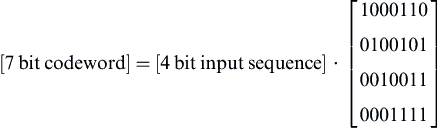
Notice that this matrix, called a generator matrix G, is simply made up of the four code words, where each row is one of the four single active bit input sequences. A simple example of generating the code word is shown below.

12.2. Linear Block Decoding
At the receiving end, we will be recovering 7-bit code words. There exists a total of 27 or 128 possible 7-bit sequence that we might receive. Only 24 or 16 of these are valid code words. If we happen to receive one of the 16 valid code words, then there has been no error in transmission, and we can easily know what 4 bit input sequence was used to generate the code word at the transmit end. But when an error does occur, we will receive one of the remaining 112 code words. We need a method to determine what error occurred, and what the original 4 bit input sequence was.
To do this, we will use another matrix, called a parity check matrix H. Let us look again at how the parity bit 2 is formed in this code, using the original parity definition.
Based on this relationship, bit 2 = 1 only when bit 6 + bit 5 + bit 3 = 1. Given the rules of binary arithmetic, we can say bit 2 + bit 6 + bit 5 + bit 3 = 0 for any valid code word. Extending this, we can say this about any valid code word:
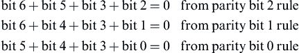
This comes from the earlier definition of the parity bit relationships we used to form the generator matrix. We can represent the three equations above in the form of parity generation matrix H.

As a quick arithmetic check, G·HT must equal zero.
We can use the parity check matrix H to decode the received code word. We can compute something called a syndrome S as indicated below.
When the syndrome is zero, all three parity equations are satisfied, there is no error, a valid code word was received, and we can simply strip away the redundant parity bits from the received code word, thus recovering the input bits. When the syndrome is nonzero, it will indicate that an error has occurred. Because this is a linear code, we can consider any received code word to be the sum of a valid code word and an error vector or word. Errors occur whenever the error vector is nonzero. The leads to the realization that the syndrome depends only on the error vector and not on the valid code word originally transmitted.
In our example, the syndrome is a 3-bit word, capable of representing eight states. When S = [0,0,0], no error has occurred. When the syndrome is any other value, an error has occurred, and the syndrome will indicate in which bit position the error is located. But which syndrome value maps to which seven possible error positions in the received code word?
Let us go back to the parity relationship that exists when the S = 0.

We have our earlier example of valid code word [1101100]. The parity check matrix is as follows:

By inspection of the parity equations, we can see that syndromes with only one nonzero bit must correspond to an error in the parity bits of the received code word.
S = [1,0,0] indicates the first parity equation is not satisfied, but the second and third are true. By inspection of parity bit definitions, this must be caused by bit 2 of the received code word, as this bit alone is used to create bit 2 of the syndrome. Similarly, an error in bit 1 in the received code word creates the syndrome [0,1,0], and error in bit 0 in the received code word creates the syndrome [0,0,1].
An error in bit 3 of the received code word will cause a syndrome of [1,1,1], as this bit appears in all three parity equations. Therefore, we can map the syndrome value to specific bit positions where an error has occurred.
S = [0,0,0] → no error in received code word
S = [0,0,1] → error in bit 0 of received code word
S = [0,1,0] → error in bit 1 of received code word
S = [0,1,1] → error in bit 4 of received code word
S = [1,0,0] → error in bit 2 of received code word
S = [1,0,1] → error in bit 5 of received code word
S = [1,1,0] → error in bit 6 of received code word
S = [1,1,1] → error in bit 3 of received code word
The procedure to correct errors is to multiply the received code word by HT, which gives S. The value of S indicated the position of error in the received code word to be corrected. This can be illustrated with an example.
Suppose we receive a code word [1111100]. We calculate the syndrome.
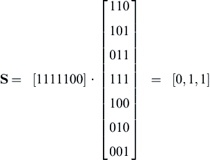
This syndrome indicates an error in bit 4. The corrected code word is [1101100], and the original 4 bit input sequence 1,1,0,1, which is not the 1,1,1,1 of the received code word.
12.3. Minimum Coding Distance
A good question is what happens when there are two errors simultaneously. Hamming codes can only detect and correct one error per received code word. The amount of detection and correction a code can perform is related to something called the minimum distance. For Hamming codes, the minimum distance is three. This means that all the transmitted code words have at least 3 bits different from all the other possible code words. Recall that in our case, we have 16 valid code words out of 128 possible sequences. These are given below as follows:
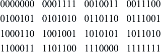
Each of these code words has 3 or more bit differences from the other 15 code words. In other words, each code word has a minimum distance of three from neighboring code words. That is why with a single error, it is still possible to correctly find the closest code word, with respect to bit differences. With two errors, the code word will be closer to the wrong code word, again with respect to bit differences. This is analogous to trying to map a symbol in two-dimensional I-Q space to the nearest constellation point in a quadrature amplitude modulation demodulator. There are other coding methods with greater minimum distances, able to correct multiple errors. We will look at one of these next.
12.4. Convolutional Encoding
A second major class of channel codes is known as convolutional coding. The convolutional code can operate on a continuous string of data, whereas block codes operated on words. Convolutional codes also have memory—the behavior of the code depends on previous data.
Convolutional coding is implemented using shift registers with feedback paths. There is a ratio of “k” input bits to “n” output bits, as well as a constraint length “K.” The code rate is k/n. The constraint length K corresponds to the length of the shift register and also determines the length of time or memory that the current behavior depends on past inputs.
Next, we will go through a very simple convolutional coding and Viterbi decoding example. We will use an example with k = 1, n = 2, K = 3 (Fig. 12.1). The encoder is described by generator equations, using polynomial expressions to describe the linear shift register relationships. The first register connection to the XOR gate is indicated by the “1” in the equations, the second by “X,” the third by X2 and so forth. Most convolution codes have a constraint length less than 10.
The rate here is ½ as for every input bit M, there are two output bits N.

The following table shows encoder operation with the input sequence 1,0,1,1,0,0,1,0,1,1,0,1 for each clock cycle. Register is initialized to zero.
| Register Value | N1 Value | N2 Value | Time or Clock Value |
| 1 0 0 | 1 | 1 | T1 |
| 0 1 0 | 1 | 0 | T2 |
| 1 0 1 | 0 | 0 | T3 |
| 1 1 0 | 0 | 1 | T4 |
| 0 1 1 | 0 | 1 | T5 |
| 0 0 1 | 1 | 1 | T6 |
| 1 0 0 | 1 | 1 | T7 |
| 0 1 0 | 1 | 0 | T8 |
| 1 0 1 | 0 | 0 | T9 |
| 1 1 0 | 0 | 1 | T10 |
| 0 1 1 | 0 | 1 | T11 |
| 1 0 1 | 0 | 0 | T12 |

The resulting output sequence: {1,1} {1,0} {0,0} {0,1} {0,1} {1,1} {1,1} {1,0} {0,0} {0,1} {0,1} {0,0}.
Notice that the output N1j and N2j are both a function of the input bit Mj and the two previous input bits Mj−1 and Mj−2. The previous K−1 bits, Mj−1 and Mj−2, form the state of the encoder state diagram. As shown, the encoder will be at a given state. The input bit Mj will cause a transition to another state at each clock edge, or Tj. Each state transition will result in an output bit pair N1j and N2j. Only certain state transitions are possible. Transitions due to a 0 bit input are shown in dashed lines, and transitions due to a 1 bit are shown in solid lines. The output bits shown at each transition are labeled on each transition arrow in Fig. 12.2.
Now, let us trace the path of the input sequence through the trellis using Fig. 12.3, and the resulting output sequence. This will help us gain the insight that the trellis is representative of the encoder circuit, as use of the trellis will be a key in Viterbi decoding. The highlighted lines show the path of input sequence. The trellis diagram covers from states 0 through 12. It is broken into three sections (A, B, C) in order to fit on the page.

By tracing the highlighted path through the trellis, you can see that the output sequence is the same as our results when computing using the shift register circuit. For constraint length K, we will have (K−1)2 states in our trellis diagram. Therefore, with K = 3 in our design example, we have four possible states. For a more typical K = 6 or K = 7 constraint length, there would be 32 or 64 states respectively; however, this is too tedious to try to diagram.
12.5. Viterbi Decoding
The decoding algorithm takes advantage of the fact that only certain paths through the trellis are possible. For example, starting from state 00, the output on the next transition must be either 0,0 or 1,1 resulting in the next state being either 0,0 or 1,0 respectively. The output of 1,0 or 0,1 is not possible, and if this sequence occurs, then an error must be present in the received bit sequence.
We will first look at Viterbi decoding using the sequence given in the last section as our example. Keep in mind that when decoding, the input data is unknown (whether a “dashed” or “solid” transition), but the output (received) data is known. The job of the decoder is to correctly recover the input data using possibly corrupted received data. The decoder does assume we start from a known state (Mj−1, Mj−2 = 0, 0).
We are going to do this by computing the difference between the received data pair, and the transition output for each possible state transition. We will keep track of this cost for each transition. Once we get further into the trellis, we can check this cumulative cost entering each of the possible states at each transition, and eliminate the path with the higher cost. In the end, this will yield that lowest-cost valid path (or valid path closest to our received sequence). As always, the best way to get a handle on this is through an example. First, we will look at the cost differences with a correct received sequence (no errors) and then one with errors present. In Fig. 12.4, the figures on each transition arrow are the absolute difference (Δ) between the two received bits and the encoder output generated by that transition (as shown on the encoding trellis diagram above).


Notice that the cumulative Δ is equal to zero as we follow the path the encoder took (solid highlighted) to generate the received sequence. But also notice two other paths that can arrive at the same point (dashed highlighted) which have a nonzero cumulative Δ. The cumulative cost of each these paths is 5. The idea is to find the path with the least cumulative Δ or difference from the received sequence. If we were decoding, we can then recover the input sequence by following the zero cost (solid highlighted) path. The dashed arrows indicate a “zero” input bit, and the solid arrows indicate a “one” input bit. The sequence recovered is therefore 1, 0, 1, 1. Notice that this sequence matches the first 4 bits input to the encoder. This is called “maximum likelihood decoding.”
This is all well and good, but as the trellis extends further into time, there are too many possible paths merging and splitting to calculate the cumulative costs. Imagine having 32 possible states, rather than the 4 in our example, and a trellis extending to hundreds of transitions. What the Viterbi algorithm will do is to remove, or prune, less likely paths. Whenever two paths enter the same state, the path having the lowest cost is chosen. The selection of lowest cost, or surviving path, is performed for all states at each transition (excluding some states at beginning and end, when the trellis is either diverging to converging to a known state). The decoded advances through the trellis, eliminating the higher cost paths, and at the end, will backtrack along the path of cumulative least cost to extract the most likely sequence of received bits. In this way, the code word, or valid sequence most closely matching the actual received sequence (which can be considered a valid code sequence plus errors) will be chosen.
Before proceeding further, we need to consider what happens at the end of the sequence. To backtrack after all the paths costs have been computed and the less likely paths pruned, we need to start backtracking from a known state. To achieve this, K−1 zeros are appended to in the input bit sequence entering the encoder. This guarantees that the last state in the encoder and therefore the decoder trellis, must be the zero state (same state as we start from, as the encoder shift register values are initialized to zero). So we will add K−1 or two zeros to our input sequence, shown in bold below, and use in our Viterbi decoding example. The longer the bit sequence, the less impact the addition of K−1 zeros will have on the overall code rate, as these extra bits do not carry information and have to be considered as part of the “redundant bits” (present only to facilitate error correction). So our code rate is slightly less than k/n.
Input bit sequence to encoder:
Output bit sequence from encoder:
The circles identify the four higher cost paths that can be pruned at T3, based on the higher cumulative path cost (ΣΔ = sum of delta or difference from received bit sequence) (Fig 12.5). The result after pruning is shown in Figs. 12.6 and 12.7 as follows:


Next, the higher cost paths (circled) are pruned at T4, again eliminating half of the paths again. The path taken by the transmitter encoder is again highlighted, at zero cumulative cost as there are no receive errors (Fig 12.8).
Owing to the constant pruning of the high-cost paths, the cumulative costs are not higher than 3 so far (Fig 12.9).
Next, we have the K−1 added bits to bring the trellis path to state 0 (Fig 12.10).
We know, due to the K−1 zeros added to the end of the encoded sequence, that we must start at state 0 at the end of the sequence, at T14.
We can simply follow the only surviving path from state 0,0 at T14 backwards, as highlighted (Fig. 12.11). We can determine the bit sequence by the color of the arrows (dashed for 0, solid for 1) (Fig.12.12). In a digital system, a 0 or 1 flag would be set for each of the four states at each Tj whenever a path is pruned, identifying the original bit Mj as 0 or 1 associated with the surviving transition.
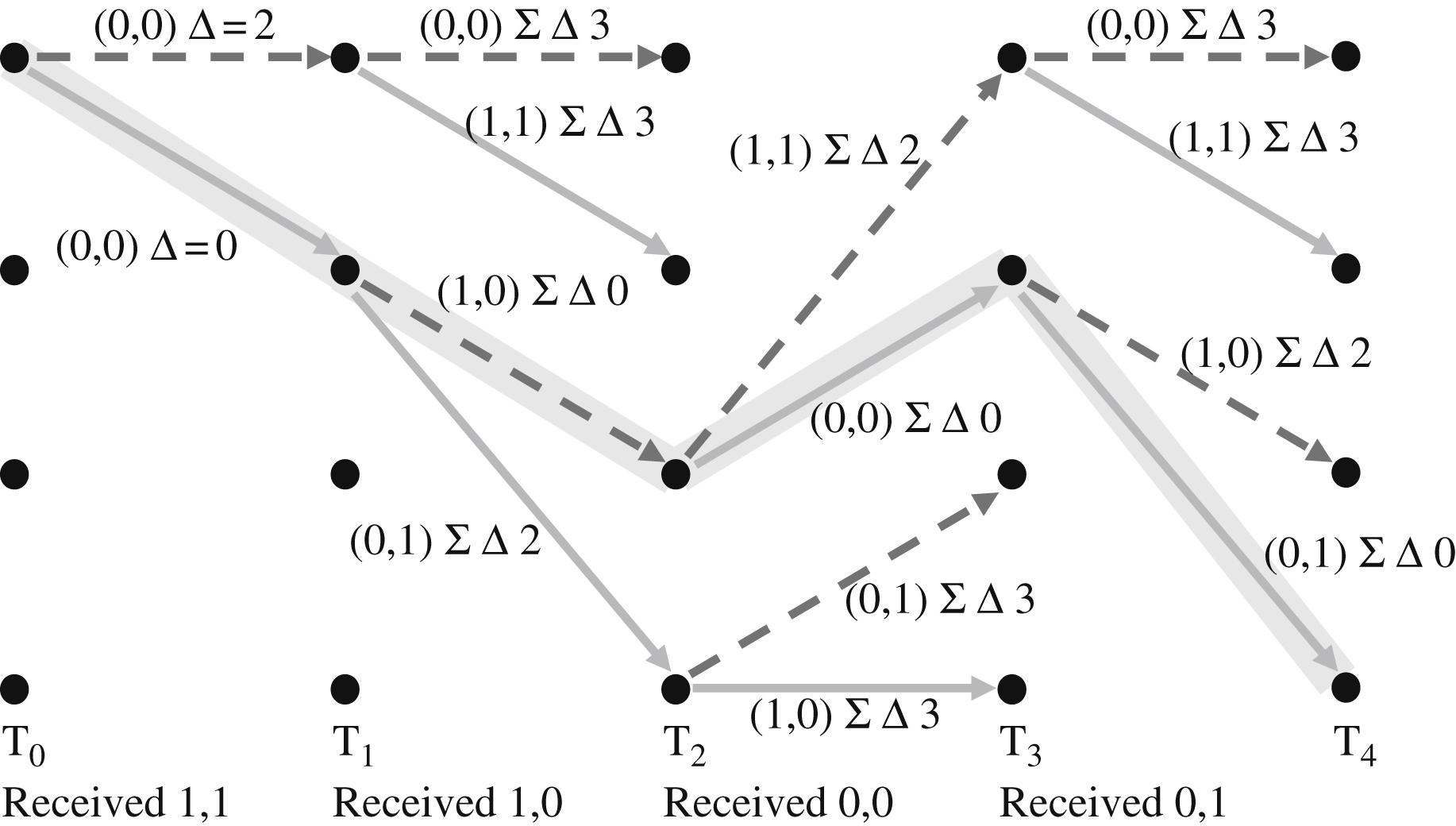


Now let us reexamine what happens in the event of receive bit errors (indicated in bold in Fig. 12.13). We will assume that there is a bit error at transition T8 and T10. The correct path (generated by encoder) through the trellis is again highlighted. Note how the cumulative costs change and the surviving paths change. However, in the end, the correct path is the sole surviving path that reaches the end point with the lowest cost.


When we had no errors, we found that all of the competing paths had different costs, and we would always prune away the higher cost path. However, in the presence of errors, we will occasionally have paths of equal cost. In these cases, it does not really matter which path we choose. For example, we can just make an arbitrary rule and always prune away the bottom path when paths of equal cumulative costs merge. And if we use soft decision decoding, which will be explained shortly, the chances of equal cost paths are very low.
The path ending at state 0, at T14, has a cumulative cost of 2, as we corrected two errors along this path. Notice that some of the pruned paths are different than the no-error Viterbi decoding example, but the highlighted path that is selected is the same in both cases. The Viterbi algorithm is finding the most likely valid encoder output sequence in the presence of receive errors and is able to do so efficiently because it prunes away less likely (higher cost) paths continuously at each state where two paths merge together.
12.6. Soft Decision Decoding
Another advantage of the Viterbi decoding method is that it supports a technique called “soft decision.” Recall from the Chapter 9 on Complex Modulation that data is often modulated and demodulated using constellations. During the modulation process, the data is mapped to one of several possible constellation points. Demodulation is the process of mapping the received symbol to the closest constellation point. This is also known as “hard decision” demodulation. However, suppose instead of having the demodulator output at the closet constellation point, it outputs the location of the received symbol relative to the constellation points. This is also known as “soft decision” demodulation.
For example, in the constellation in Fig. 12.14, imagine that we receive the symbol labeled S1, S2, S3,and S4. We will demodulate these symbols as follows:

Basically, we are telling the Viterbi decode how sure we are of the correct demodulation. Instead of giving a yes or no at each symbol, we can also say “maybe” or “pretty sure.” The received signal value in the trellis calculation is now any value between 0 and 1 inclusive. This is then factored into the path costs, and the decision on which merged path to prune away.
Simulation and testing have shown over 2 dB improvement in coding gain when using soft decision (16 levels, or 4 bits) compared to hard decision (2 levels, or single bit) representation for the decisions coming from the demodulator. The additional Viterbi decoding complexity for soft decoding is usually negligible.
There are many other error-corrective codes besides the two simple ones we have presented here. Some common codes used in industry are Reed Solomon, BCH, and Turbo decoding. LDPC is another emerging coding technique, which promises even higher performance at a cost of much increased computational requirements. In addition, different codes are sometime concatenated to further improve performance.

12.7. Cyclic Redundancy Check
A CRC or cyclic redundancy check word is often appended at the end of a long string or packet of data, prior to the error-correcting encoder. The CRC word is formed by taking all the data words and exclusive OR gate (EXOR) each word together. For example, the data sequence might be 1024 bits, organized as 64 words, each 16 bits. This would require 16-1 EXOR word operations in a DSP or in hardware to form the 16 bit CRC word. This function is analogous to that of a parity check bit for a single digital word being stored and accessed from DRAM memory.
At the conclusion of the error-decoding process, the recovered input stream can again be partitioned in words and EXORed together, and the result compared to the recovered CRC word. If they match, then we can be assured with very high probability that the error correction was successful in correcting any error in transmission. If not, then there were too many errors to be corrected, and the whole data sequence or frame can be discarded. In some cases, there is a retransmission facility built into the higher level communication protocol for these occurrences, and in others, such as a voice packet in mobile phone system, the data is “real time,” so alternate mechanisms of dealing with corrupt or missing data are used.
12.8. Shannon Capacity and Limit Theorems
No discussion on coding should be concluded without at least a mention of the Shannon capacity theorem and Shannon limit. The Shannon capacity theorem defines the maximum amount of information, or data capacity, which can be sent over any channel or medium (wireless, coax, twister pair, fiber etc.).
where
C is the channel capacity in bits per second (or maximum rate of data)
B is the bandwidth in Hz available for data transmission
S is the received signal power
N is the total channel noise power across bandwidth B
What this says is that higher the signal-to-noise (SNR) ratio and more the channel bandwidth, the higher the possible data rate. This equation sets the theoretical upper limit on data rate, which of course is not fully achieved in practice.
It does not make any limitation on how low the achievable error rate will be. That is dependent on the coding method used.
As a consequence of this, the minimum SNR required for data transmission can be calculated. This is known as the Shannon limit, and it occurs as the available bandwidth goes to infinity.
where
Eb is the energy per bit
N0 is the noise power density in Watts/Hz (N = B N0)
If the Eb/N0 falls below this level, no modulation method or error-correction method will allow data transmission.
These relationships define maximum theoretical limits, against which the performance of practical modulation and coding techniques can be compared against. As newer coding methods are developed, we are able to get closer and closer to the Shannon limit, usually at the expense of higher complexity and computational rates.
..................Content has been hidden....................
You can't read the all page of ebook, please click here login for view all page.