Chapter 9
Complex Modulation and Demodulation
Abstract
This chapter discusses the techniques of complex modulation and demodulation through an intuitive approach. Modulation as a process in which data is mapped into symbols. The use of modulation constellations leads the problem of avoiding intersymbol interference, or the avoidance of symbols overlapping one another in time. The raised cosine filter is introduced as the solution, which have been plotted for several roll-off factors. The combined transmitter and receiver affects of the raised cosine filter are shown, leading to use of the square root of raised cosine filter.
Keywords
Intersymbol interference; Pulse-shaping filter; Quadrature phase shift keying; Raised cosine filter; Roll-off factor
We are going to try to take an unusual approach here. The normal explanations on this topic are heavily based on mathematics and equations. Here, we will try to take an almost entirely intuitive approach, based on examples. There will be no attempt to establish any mathematical foundation or to calculate performance.
Modulation is the process of taking information bits and mapping them to symbols. The sequence of symbols is then filtered to produce a baseband waveform, with the desired spectral properties. This baseband waveform or signal is then upconverted to a carrier frequency, which can be transmitted over the air, through coaxial cable, through fiber or some other medium. The key idea here is the concept of a symbol.
9.1. Modulation Constellations
We are going to use a common modulation method, known as QPSK (quadrature phase shift keying), as our first example. Do not let the technically sounding names of these different modulations confuse you. We will talk about what these names mean later. With QPSK, every two input bits will map to one of four symbols, as shown below in Fig. 9.1.

The bitstream of zeros and ones input to the modulator is converted into a stream of symbols. Each symbol is represented as the coordinates of a location in the I-Q plane. In QPSK, there are four possible symbols, arranged as shown. Since there are four symbols, then the input data is arranged as groups of 2 bits, which are mapped to the appropriate symbol. The arrangement of symbols in the I-Q plane is also called the constellation (See Table 9.1).
Another common modulation scheme is known as 16-QAM (quadrature amplitude modulation), which has 16 symbols, arranged as shown in Fig. 9.2. Again, do not worry about the name of the modulation. Since we have 16 possible symbols, each symbol will map to 4 bits. To put it another way, in QPSK, each symbol carries 2 bits of information, while in 16-QAM, each symbol carries 4 bits of information.
We can easily see that the 16-QAM is the more efficient modulation method. In this chapter, we are going to pick a convenient symbol rate and reference our discussion to this symbol rate. But this is an arbitrary choice on my part, and systems are designed with symbol rates ranging from a few kHz to hundreds of MHz. We will decide to transmit symbols at a rate of 1 MHz, or 1 MSPS (million symbols per second). Then our system, if using the 16-QAM modulation, will be able to send 4 Mbits/s. If instead QPSK is used in this system, it will able to send only 2 Mbits/s. We could also use an even more efficient constellation, 64-QAM. Since there are 64 possible symbols, arranged as eight rows of eight symbols each, then each symbol carries 6 bits of information, and support a data rate of 6 Mbits/s. This is shown in the table below for a few sample constellation types (See Table 9.2).
Table 9.1
Quadrature Phase Shift Keying Symbol to Bit Mapping
| Input Bit Pair | Symbol Location on Complex Plane | I Value | Q Value | Symbol Value (Same as Location on Complex Plane |
| 0, 0 | 1 + j | 1 | 1 | I + jQ => 1 + j |
| 0, 1 | 1 − j | 1 | −1 | I + jQ => 1 − j |
| 1, 0 | −1 + j | −1 | 1 | I + jQ => −1 + j |
| 1, 1 | −1 − j | −1 | −1 | I + jQ => −1 − j |


The frequency bandwidth is determined mainly by the symbol rate. A QPSK signal at 1 MSPS will require about the same bandwidth as a 16-QAM signal at 1 MSPS. Notice the 16-QAM modulator is able to send twice the data within this bandwidth, compared to the QPSK modulator. There is a trade-off, however. As we increase the number of symbols, it becomes more and more difficult for the receiver to detect which symbol was sent. If receiver needs to choose among 16 possible symbols that could have been transmitted, rather than choose from among four possibilities, it is more likely to make errors. The level of errors will depend on the noise and interference present in the receive signal, the strength of the receive signal, and how many possible symbols the receiver must select from. In cellular systems, there are often high levels of interfering noise or weak signals due to buildings or other objects block the transmission path. In this situation, it is often preferable to use a simple constellation, such as QPSK. Even with a weak signal, the receiver can usually make the correct choice of four possible symbols. Other systems, such as microwave radio systems, usually have directional receive and transmit antennas facing each other from building roofs or mountaintops. Because of this, the interfering noise level is usually very low, and complex constellations such as 64-QAM or 256-QAM can be used. Assuming the receiver is able to make the correct choice from among 64 symbols, which allows three times more bits to be encoded into each symbol, resulting in a 3× higher data rate. Recently, sophisticated communication systems such as LTE and WiMax have been introduced, which allow the transmitter to dynamically switch between constellation types depended on quality of reception the receiver experiences.

9.2. Modulated Signal Bandwidth
Now that we understand what a constellation is, we still need to discuss some of the steps in taking this set of constellation points and transmitting this over some medium to a receiver. Let us take a look at a QPSK constellation, with transmission rate of 1 MSPS. The baseband signal is two dimensional, so must be represented with two orthogonal components, which are by convention denoted I and Q.
Let us consider a sequence of 5 QPSK symbols, at time t = 1,2,3,4, and 5 respectively. First, let us look at the sequence in the two dimensional complex constellation plane. It will appear as a signal trajectory moving from one constellation point to another over time.
We can also look at the I and Q signals individually, plotted against time in Fig. 9.4. We can take this two-dimensional signal, and plot each component separately. In actuality, the I and Q baseband signals are generated as two separate signals, and later combined together with a carrier frequency to form a single passband signal (See Fig 9.3). This is discussed in Chapter 11.
Notice the sharp transitions of the I and Q signals at each symbol. Intuitively, we know that a sharp transition requires the signal to have high-frequency content. A signal that is of low frequency can change only slowly and smoothly.
The high-frequency content of these I and Q signals can cause problems, because in most systems, it is important to minimize the frequency content or bandwidth of the signal. Remember the early discussion on frequency response, where a low-pass filter removes fast transitions or changes in a signal (or eliminates the high frequency components of that signal). If the frequency response of the signal is reduced, this is the same as reducing its bandwidth. The smaller the bandwidth of the signal, the more signal channels and therefore capacity can be packed into a given amount of frequency spectrum. Thus the channel bandwidth is often carefully controlled.


A simple example is FM radio. Each station, or channel, is located 200 kHz from its neighbor. That means that each station has 200 kHz spectrum or frequency response it can occupy. The station on 101.5 is actually transmitting with a center frequency of 101.5 MHz. The channels on either side transmit with center frequencies of 101.3 and 101.7 MHz. Therefore it is important to restrict the bandwidth of each FM station to within ± 100 kHz, which ensure it does not overlap or interfere with neighboring stations. As we know by now, one way to restrict the bandwidth of a signal is to use a filter.
In this discussion, we are assuming that a given signal's frequency response, or spectrum, can be moved up or down the frequency axis at will. This is true, and is called up or down conversion, and will be discussed in Chapter 11.
9.3. Pulse-Shaping Filter
To accomplish this frequency limiting of the modulated signal, one needs to pass the I and Q signals through a low pass filter. This filter is often called a pulse-shaping filter, and it determines the bandwidth of the modulated signal. But it is not quite that simple. We need to consider what the filter does to the signal in the time domain as well.
Suppose that we use an ideal low pass filter. Let us use our example where symbols are generated at a rate R of 1 MSPS. The period T is the symbol duration, and equal to 1 μs in our example. The relationship between the rate R and symbol period T is:
If we alternate with positive and negative I and Q values at each sample interval (this is the worst case in terms of high-frequency content), the rate of change will be 500 kHz. So we will start with a low-pass filter with passband of 500 kHz (See Fig. 9.5).
This filter will have the sinc impulse or time response. The impulse response is shown in red. It has zero crossings at intervals of T seconds and decays slowly. A very long filter is needed to approximate the sinc response. The impulse response of the symbols immediately preceding and following the center symbol is in Fig. 9.6 shown below. The actual transmitted signal will be the sum of all the symbols impulse response (we are just showing three symbols here). If the I or Q sample has a negative value for a particular symbol, then the impulse response for that symbol will be inverted from what is shown below.


Think for a moment about the job of the receiver. The receiver is sampling the signal at T intervals in time to detect the symbol values. It must sample at the T intervals shown on the time axis above (leave aside for now the question of how the receiver knows exactly where to sample). At time t = −T, the receiver will be sampling the first symbol. Notice how the two later symbols have zero crossings at t = −T, and so have no contribution at this instant. At t = 0, the receiver will be sampling the value of the second symbol. Again, the other symbols, such as first and third adjacent symbols, have zero crossings at t = 0 and have no contribution. If we were to reduce the bandwidth of the filter to less than 500 kHz (R/2) then in the frequency domain, these pulses would widen (remember that the narrower the frequency spectrum, the longer the time response, and vice versa). This is shown below in Fig. 9.7 if the Fcutoff of the pulse shaping filter is narrowed to 250 kHz or R/4.
In this case, notice how at time t = 0, the receiver will be sampling contributions from multiple pulses. At each sampling point of t equal to …−3T, −2T, −T, 0, T, 2T … the signal is going to have contributions from many nearby symbols, preventing detection of any specific symbol. This phenomenon is known as intersymbol interference (ISI) and shows that to transmit symbols at a rate R, one needs to have at least R Hz (or 1/T Hz) in the passband frequency spectrum. At baseband, the equivalent two dimensional (complex) spectrum is from −R/2 to +R/2 Hz to avoid creating ISI. Therefore to transmit a 1 MSPS signal over the air, at least 1 MHz of RF frequency spectrum will be required. The baseband filters will need a cutoff frequency of at least 500 kHz.
Notice that the frequency spectrum or bandwidth required depends on the symbol rate, not the bit rate. We can have a much higher bit rate, depending on the constellation type used. For example, each 256-QAM symbol carries 8 bits of information, while a QPSK symbol carries only 2 bits of information. But if they both have a common symbol rate, both constellations require the same bandwidth.

We still have two problems, however. One is that the sinc impulse response decays very slowly, and so will take a long filter (many multipliers) to implement. The second is that although the response of the other symbols does go to zero at the sampling time when t = N·T, where N is any integer, we can see visually that if our receiver samples just a little bit to either side, the adjacent symbols will contribute. This makes the receiver symbol detection performance very sensitive to our sampling timing.
Ideally, what we want is an impulse response that still goes to zero at intervals of T, but decays faster, and has lower amplitude lobes or tails. This way, if we sample a bit to one side of the ideal sampling point, the lower amplitude tails will make the unwanted contribution of the neighboring symbols smaller. By making the impulse response decay faster, we can reduce the number of taps and therefore multipliers, required to implement the pulse shaping filter.
9.4. Raised Cosine Filter
There is a type of filter commonly used to meet these requirements. It is called the “raised cosine filter”, and it has an adjustable bandwidth, controlled by the “roll-off” factor. The trade-off will be that as bandwidth of the signal will become a bit wider, more frequency spectrum will be required to transmit the signal (See Table 9.3).
The following table summarizes the raised cosine response shown in Fig. 9.8 for different roll-off factors.
In Fig. 9.8 above, the frequency response of the raised cosine filter is shown. To better see the passband shape, it is plotted linearly, rather than logarithmically (dB). It has a cutoff frequency of 500 kHz, the same as our ideal low-pass filter. A raised cosine filter response is wider than the ideal low-pass filter, due to the transition band. This excess frequency bandwidth is controlled by a parameter called the “roll-off” factor. The frequency response is plotted for several different roll-off factors. As the roll-off factor gets closer to zero, the transition becomes steeper, and the filter approaches the ideal low-pass filter.
Table 9.3
Raised cosine Roll-Off Factor Characteristics
| Roll-Off Factor | Label | Commentsa |
| 0.10 | A | Requires long impulse response (high multiplier resources), has small frequency excess bandwidth of 10% |
| 0.25 | B | A commonly used roll-off factor, excess bandwidth of 25% |
| 0.50 | C | A commonly used roll-off factor, excess bandwidth of 50% |
| 1.00 | D | Excess bandwidth of 100%, never used in practice |

The impulse response of the raised cosine filter is shown above. Fig. 9.9 shows the filter impulse response, and Fig. 9.10 zooms in to better show the lobes of the filter impulse. Again, it is plotted for several different roll-off factors. It is similar to the sinc impulse response in that it has zero crossings at time intervals of T (as this is shown in sample domain, rather than time domain, it is not readily apparent from the diagram).
As the excess bandwidth is reduced to approach the ideal low-pass filter frequency response, the lobes in the impulse response become higher, approaching the sinc impulse response. The signal with the smaller amplitude lobes has a larger excess bandwidth or wider spectrum (See Fig. 9.9).
Let us review this idea of pulse-shaping filter again, in light of the Figs. 9.9 and 9.10. We need a pulse shaping filter which will have a zero response at intervals of T in time so that a given symbol's pulse response will not have a contribution to the signal at the sampling times of the neighboring symbols. We would also like to minimize the height of the lobes of the impulse (time) response and have it decay quickly, as to reduce our sensitivity to ISI, if the receiver does not sample precisely at the correct time for each symbol. As the roll-off factor increases, we can see this is exactly what happens in the figures (signal “D”). The impulse response goes to zero very quickly, and the lobes of the filter impulse response are very small. On the other hand, we have a frequency spectrum, which is excessively wide. A better compromise would be a roll-off factor somewhere between 0.25 and 0.5 (signals “B” and “C”). Here, the impulse response decays relatively quickly with small lobes, requiring a pulse-shaping filter with small number of taps, while still keeping the required bandwidth reasonable.


The roll-off factor controls the compromise between:
• spectral bandwidth requirement,
• length or number of taps of pulse shaping filter, and
• receiver sensitivity to ISI.
Another significant aspect of the pulse-shaping filter is that it is always an interpolating filter. In our figures, this is shown as a four times interpolation filter. If you look carefully at the impulse response in the Fig. 9.10, you can see that the zero crossing are every four samples. This corresponds to t = N·T in the time domain, due to the 4× interpolation.
The pulse-shaping filter must be an interpolating filter, as the I and Q baseband signals must meet the Nyquist criterion. In this example, the symbol rate is 1 MSPS. If we use a high roll-off factor, the baseband spectrum of the I and Q signals can be as high as 1 MHz. So we require a minimum sampling rate of 2 MHz or twice the symbol rate. Therefore, the pulse-shaping filter will need to interpolate by at least a factor of two and is often interpolated quite a bit higher than this, for reasons we will discuss in the digital upconversion chapter.
Once we have our pulse shaped and interpolated I and Q baseband digital signals, we can use digital to analog converters to create the analog I and Q baseband signals. These signals can be used to drive an analog mixer that can create a passband signal. A passband signal is a baseband signal which has been upconverted or mixed with a carrier frequency.
For example, we might use a 0.25 roll-off filter for our 1 MSPS modulator. The baseband I and Q signals will have a bandwidth of 625 kHz. If we use a carrier frequency of 1 GHz, then our transmit signal will require about 1.25 MHz of spectrum centered at 1 GHz.
So far, we have discussed the process which occurs in the transmission path. The receive path is quite similar. The signal is down converted or mixed down to baseband. Again, we will discuss this in more detail in a later chapter. The demodulation process starts with baseband I and Q signals. The receiver is more complex, as it must deal with several additional issues. First of all, there may be nearby signals that can interfere with the demodulation process. These must be filtered out, usually with a combination of analog and digital filters. The final stage of digital filtering is often the same pulse-shaping filter used in the transmitter. This is called a matched filter. The idea is that if the same filter that was used to create the signal is also used to filter the spectrum prior to sampling, we can maximize the amount of signal energy used in the detection (or sampling process). There is a bit of mathematics to prove this, so we will just take it at face value. Due to this idea of using the same filter in the transmitter and receiver, the raised cosine filter is usually modified to a square root raised cosine filter. The frequency response of the raised cosine filter is modified to be the square root of the amplitude across the passband. This also modifies the impulse response as well. This is shown in the figures below, for the same roll-off factors (See Figs. 9.11 and 9.12).


Since the signal passes through both filters, the net frequency response is the raised cosine filter. After passing through the receive pulse-shaping (also called matched) filter, the signal is sampled. Using the sampled I and Q value, the receiver will choose the constellation point in the I-Q plane closest to the sampled value. The bits corresponding to that symbol are recovered, and if all went well, the receiver has chosen the same symbol point selected by the transmitter. We have very much simplified this whole process, but this is the essence of digital communications.
We can see why it will be easier to have errors when transmitting 64-QAM as compared to QPSK. The receiver has 64 closely spaced symbols to select from in the case of 64-QAM, whereas in QPSK, there are only four widely spaced symbols to select from. This makes 64-QAM systems much more susceptible to ISI, noise or interference. You might think, let us transmit the 64-QAM signal with higher power, as to spread the symbols further apart. This is an effective, but very expensive way, to mitigate the noise and interference which prevents correct detection of the symbol at the receiver. Also, the transmit power is often limited by the regulatory agencies, or the transmitter may be battery powered or have other constraints.
The receiver also has a number of other problems to contend with. We assumed that we always sample at the correct instant in time when one symbol has a nonzero value in the signal. The receiver must somehow determine this correct sampling time, usually by a combination of trial and error during initial part of the reception, and sometimes by having the transmitter send a predetermined (or training) sequence known by both transmitter and receiver. This process is known as acquisition, where the receiver tries to fine-tune the sampling time, the symbol rate, the exact frequency and phase of the carrier and other parameters, which may be needed to demodulate the received signal with a minimum of errors. And once all this information is determined, it must still be tracked, to account for differences in transmit and receive clocks, Doppler shifts due to relative motion between the receiver and transmitter, and changes in the path the signal takes from transmitter to receiver, causing various reflections, distortions, and attenuations.
These problems are what make digital receivers so difficult and interesting to work with. Unfortunately, there is usually a lot of mathematics associated with most receiver algorithms and methods, so we will not go into this in any depth. But later chapters will describe the basic principles of several common types of digital communication systems.
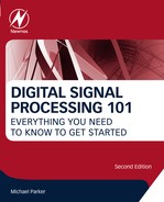
Below in Figs. 9.13 and 9.14 are plots from both a 16-QAM and 64-QAM constellation after being sampled by an actual digital receiver. Each receiver signal has the same average energy. This is from a WiMax wireless system, operating in the presence of noise. But the receiver does manage to do a sufficiently good job at detection so that each of the constellation points is clearly visible. But we can imagine that as the receiver noise level increases, the constellation samples would quickly start to drift together on the 64-QAM constellation, and we would be unable to accurately determine to which constellation point a given symbol should map to. The 16-QAM system is more robust in the presence of additive noise and other impairments, compared to the 64-QAM.
The modulation and demodulation (modem) ideas presented in this chapter are used in most digital communication systems, including satellite, microwave, cellular (OFDMA, CDMA, and TDMA), wireless LAN (OFDM), DSL, fax, and data dialup modems. Actually, the lowly dialup modem is among the most complicated of all—a V.34 modem can have over 1000 constellation points.
Hopefully, by now the name conventions of the modulation methods is starting to make more sense. In QPSK, all four symbols have the same amplitude. The phase in the complex plane is what distinguishes the different symbols, each of which is located in a different quadrant. For QAM, the amplitude and phase of the symbol is needed to distinguish a particular symbol.
In general, communication systems are full of trade-offs. The most important comes from a famous theorem developed by Claude Shannon, which gives the maximum theoretical data bit rate that can be communicated over a communications channel depending upon bandwidth, transmit power, and receiver noise level. It gives the maximum data rate that can be sent over a channel or link with a given noise level and bandwidth.

This is known as the Shannon limit and is somewhat analogous to the speed of light, which can be approached with ever increasing amounts of cleverness and effort, but can never be exceeded. This will be discussed further in the chapter on error correction codes.
..................Content has been hidden....................
You can't read the all page of ebook, please click here login for view all page.