
Chapter 24
DCT, Entropy, Predictive Coding, and Quantization
Abstract
In this chapter, we will discuss some of the basic concepts used in data compression, including video and image compression. Up until now, we have considered only uncompressed video formats, such as RGB or YCrCb, where each pixel is individually represented (although this is not strictly true for 4:2:2 or 4:2:0 forms of YCrCb). However, much greater levels of compression are possible with little loss of video quality. Reducing the data needed to represent an individual image or a sequence of video frames is very important when considering how much storage is needed on a camera flash chip or computer hard disk, or the bandwidth needed to transport cable or satellite television, or stream video to a computer or handheld wireless device.
Keywords
Decibel; Differential encoding; Entropy; Huffman coding; Lossless compression; Lossy compression; Markov source; Predictive coding; Quantization
In this chapter, we will discuss some of the basic concepts used in data compression, including video and image compression. These concepts may seem unrelated, but will come together in the following chapter. Up until now, we have considered only uncompressed video formats, such as RGB or YCrCb, where each pixel is individually represented (although this is not strictly true for 4:2:2 or 4:2:0 forms of YCrCb). However, much greater levels of compression are possible with little loss of video quality. Reducing the data needed to represent an individual image or a sequence of video frames is very important when considering how much storage is needed on a camera flash chip or computer hard disk, or the bandwidth needed to transport cable or satellite television, or stream video to a computer or handheld wireless device.
24.1. Discrete Cosine Transform
The discrete cosine transform, or DCT is normally used to process two dimensional data, such as an image. Unlike the DFT or FFT that operates on one dimensional signals, which may have real and quadrature components., the DCT is usually used as an image presented by a rectangular array of pixels, which is a real signal only. When we discuss frequency, it will be how rapidly the sample values change. With the DCT, we will be sampling spatially across the image in either the vertical or horizontal direction.
The DCT is usually applied across an N by N array of pixel data. For example, if we take a region composed or 8 by 8 pixels, or 64 pixels total, we can transform this into a set of 64 DCT coefficients, which is the spatial frequency representation of the 8 × 8 region of the image. This is very similar to what we say in the DCT. However, instead of expressing the signal as a combination the complex exponentials of various frequencies, we will be expressing the image data as a combination of cosines of various frequencies, in both vertical and horizontal dimensions.
Now recall in the discussion on DFT, that the DFT representation is for a periodic signal or one that is assumed to be periodic. Now imagine connecting a series of identical signals together, end to end. Where the end of the sequence connects to the beginning of the next, there will be a discontinuity, or a step function. This will represent high frequency.
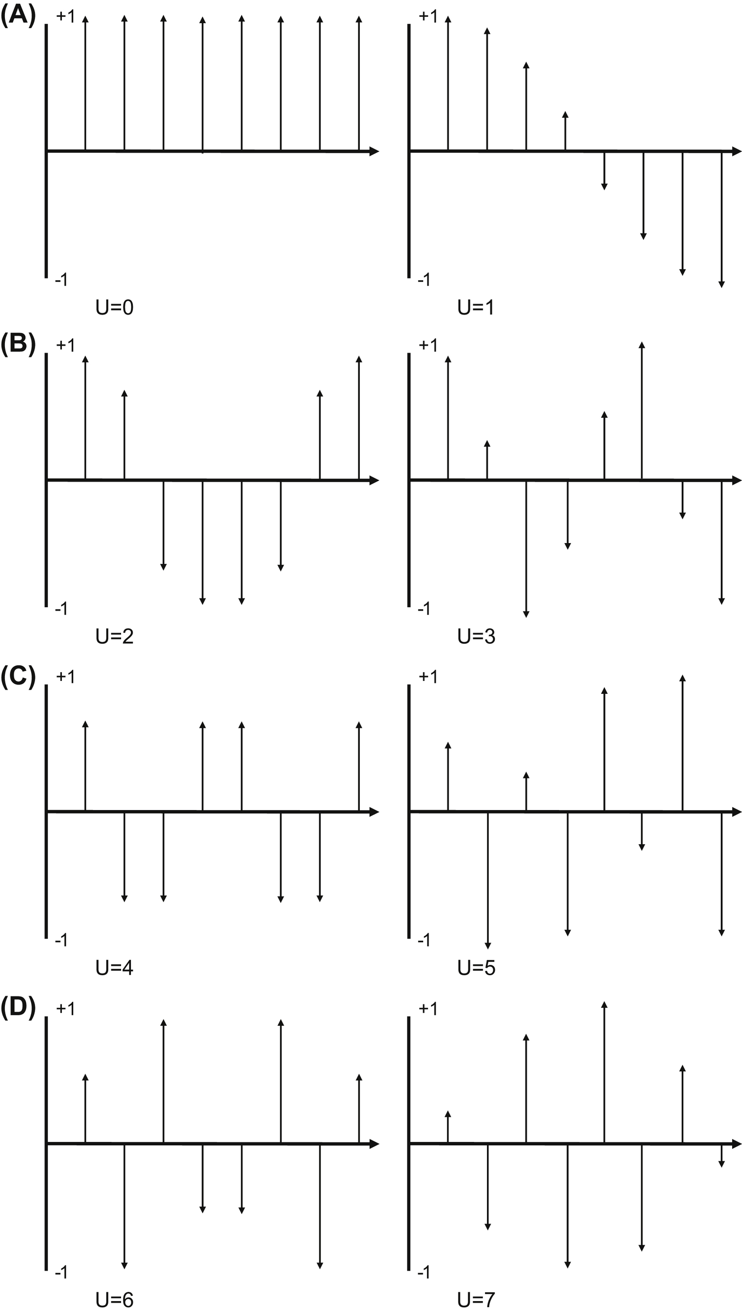
For the DCT, we make an assumption that the signal is folded over on itself. So an 8 long signal depicted becomes 16 long when appended as flipped. This 16 long signal is then symmetric about the midpoint. This is the same property of cosine waves. A cosine is symmetric about the midpoint, which is at π (since the period is from 0 to 2π). This property is preserved for higher frequency cosines, that only 8 of the 16 samples are needed as shown by the figures below, showing the sampled cosine waves. The waveforms in Fig. 24.1 are eight samples long, and if folded over to create 16 long sampled waveforms which will be symmetric, start and end with the same value, and has “u” cycles across the 16 samples.
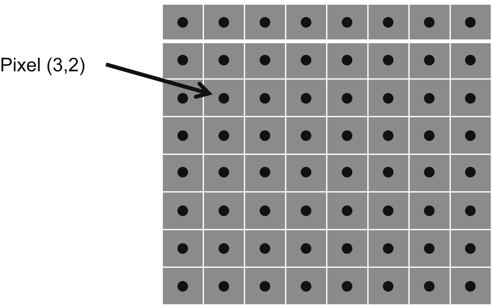
To continue requires some terminology. The value of a pixel at row x and column y is designated as f(x,y), as shown in Fig. 24.2. We will compute the DCT coefficients, F(u,v) using equations that will correlate the pixels to the vertical and horizontal cosine frequencies. In the equations, “u” and “v” correspond to both the indices in the DCT array, and the cosine frequencies as shown in Fig. 24.1.
The relationship is given in the DCT equation, shown below for the 8 × 8 size.
where
Cu = √2/2 when u = 0, Cu = 1 when u = 1…7
Cv = √2/2 when v = 0, Cu = 1 when v = 1…7
f(x,y) = the pixel value at that location
This represents 64 different equations, for each combination of u, v. For example:
Or simply the summation of all 64 pixel values divided by 8. F(0,0) is the DC level of the pixel block.
The nested summations indicate for each of the 64 DCT coefficients, we need to perform 64 multiply and adds. This requires 64 × 64 = 4096 calculations, which is very processing intensive.
The DCT is a reversible transform (provided enough numerical precision is used), and the pixels can be recovered from the DCT coefficients as shown below.
Cu = √2/2 when u = 0, Cu = 1 when u = 1…7
Cv = √2/2 when v = 0, Cu = 1 when v = 1…7
Another way to look at the DCT is through the concept of basis functions.
These tiles represent the video pixel block for each DCT coefficient. If F(0,0) is nonzero, and the rest of the DCT coefficients equal zero, the video will appear as the {0,0} tile in Fig. 24.3. This particular tile is a constant value in all 64 pixel locations, which is what is expected since all the DCT coefficients with some cosine frequency content are zero.
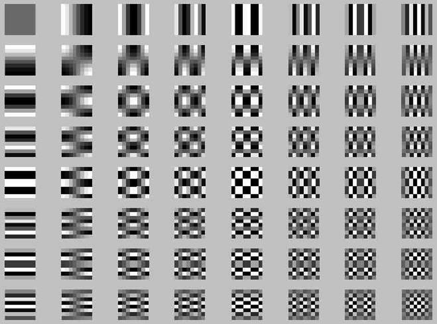
If F(7,7) is nonzero, and the rest of the DCT coefficients equal zero, the video will appear as the {7,7} tile in Fig. 24.3, which shows high frequency content in both vertical and horizontal direction. The idea is that any block of 8 × 8 pixels, no matter what the image, can be represented as the weighted sum of these 64 tiles in Fig. 24.3.
The DCT coefficients, and the video tiles they represent, form a set of basis functions. From linear algebra, any set of function values f(x,y) can be represented as a linear combination of the basis functions.
The whole purpose of this is to provide an alternate representation of any set of pixels, using the DCT basis functions. By itself, this exchanges one set of 64 pixel values with a set of 64 DCT values. However, it turns out frequently in many image blocks, many of the DCT values are near zero, or very small and can be presented with few bits. This can allow the pixel block to be presented more efficiently with fewer values. However, this representation is approximate, because when chose to minimize the bits representing various DCT coefficients, we are quantizing. This is a loss of information, meaning the pixel block cannot be restored perfectly.
24.2. Entropy
We will start with the concept of entropy. Some readers may recall from studies in thermodynamics or physics that entropy is a measure of the disorderliness of a system. Further, the second law of thermodynamics states that in a closed system, entropy can only increase and never decrease. In the study of compression, and also a related field of err correction, entropy can be thought of as the measure of unpredictability. This can be applied to a set of digital data.
The less predictable a set of digital data is, the more information it carries. Here is a simple example. Assume that a bit can be equally likely to be either 0 or 1. By definition, this will be 1 bit of data information. Now assume that this bit is known to be a 1 with 100% certainty. This will carry no information, because the outcome is predetermined. This relationship can be generalized by:
Info of outcome = log2 (1/probability of outcome) = −log2 (probability of outcome)
Let us look at another example. Suppose there is a four outcome event, with equal probability of outcome1, outcome2, outcome3, or outcome4.
Outcome 1: Probability = 0.25, encode as 00
Outcome 2: Probability = 0.25, encode as 01
Outcome 3: Probability = 0.25, encode as 10
Outcome 4: Probability = 0.25, encode as 11
The entropy can be defined as the sum of the probabilities of each outcome multiplied by the information conveyed by that outcome.
Entropy = prob (outcome1) · info (outcome1) + prob (outcome2) · info (outcome2) + … prob (outcomen) · info (outcomen)
In our simple example,
This is intuitive—2 bits is normally what would be used to convey one of four possible outcomes.
In general, the entropy is the highest when the outcomes are equally probable, and therefore totally random. When this is not the case, and the outcomes are not random, the entropy is lower, and may be possible to take advantage of this and reduce the number of bits to represent the data sequence.
Now what if the probabilities are not equal, for example:
Outcome 1: Probability = 0.5, encode as 00
Outcome 2: Probability = 0.25, encode as 01
Outcome 3: Probability = 0.125, encode as 10
Outcome 4: Probability = 0.125, encode as 11
24.3. Huffman Coding
Since the entropy in the previous example is less than 2 bits, then in theory, we should be able to convey this information in less than 2 bits. What if we encoded these events differently as shown below:
Outcome 1: Probability = 0.5, encode as 0
Outcome 2: Probability = 0.25, encode as 10
Outcome 3: Probability = 0.125, encode as 110
Outcome 4: Probability = 0.125, encode as 111
One-half the time, we would present the data with 1 bit, one-fourth of the time with 2 bits, and one-fourth of the time with 3 bits.
So this outcome can be represented with less than 2 bits, in this case 1.75 bits. The nice thing about this encoding is that the bits can be put together into a continuous bit stream and unambiguously decoded.
010110111110100….
The sequence above can only represent one possible outcome sequence.
outcome1, outcome2, outcome3, outcome4, outcome3, outcome2, outcome1…
An algorithm known as Huffman coding works in this manner, by assigning the shortest codewords (the bit-word that each outcome is mapped to, or encoded) to the events of highest probability. For example, Huffman codes are used in JPEG-based image compression. Actually, this concept was originally used in Morse code for telegraphs over 150 years ago, where each letter of the alphabet is mapped to a series of short dots and long dashes.
Common letters.
Uncommon letters.
In Morse code, the higher probability letters are encoded in a few dots or a single dash. The less likely probability letters use several dashes and dots. This minimizes, on the average, the amount of time required by the operator to send a telegraph message, and the number of dots and dashes transmitted.
24.4. Markov Source
Further opportunities for optimization arise, when the probability of each successive outcome or symbol is dependent on previous outcomes. An obvious example is that if the nth letter is a “q”, you can be pretty sure the next letter will by a “u”. Another example is that if the nth letter is a “t”, this raises the probability that the following letter will be an “h”. Data sources that have this kind of dependency relationship between successive symbols are known as Markov sources. This can lead to more sophisticated encoding schemes. Common groups of letters with high probabilities can be mapped to specific codewords. Examples are the letter pairs “st” and “tr”, or “the”.
This falls out when we map the probabilities of a given letter based on the few letters preceding. In essence, we are making predictions based on the probability of certain letter groups appearing in the any given construct of the English language. Of course, different languages, even if using the same alphabet, will have a different set of multiletter probabilities, and therefore different codeword mappings. An easy example in the United States is the sequence of letters: HAWAI_. Out of 26 possibilities, it is very likely the next letter is an “I”.
In a first order Markov source, a given symbol's probability is dependent on the previous symbol. In a second order Markov source, a given symbol's probability is dependent on the previous two symbols, and so forth. The average entropy of a symbol tends to decrease as the order of the Markov source increases. The complexity of the system also increases as the order of the Markov source increases.
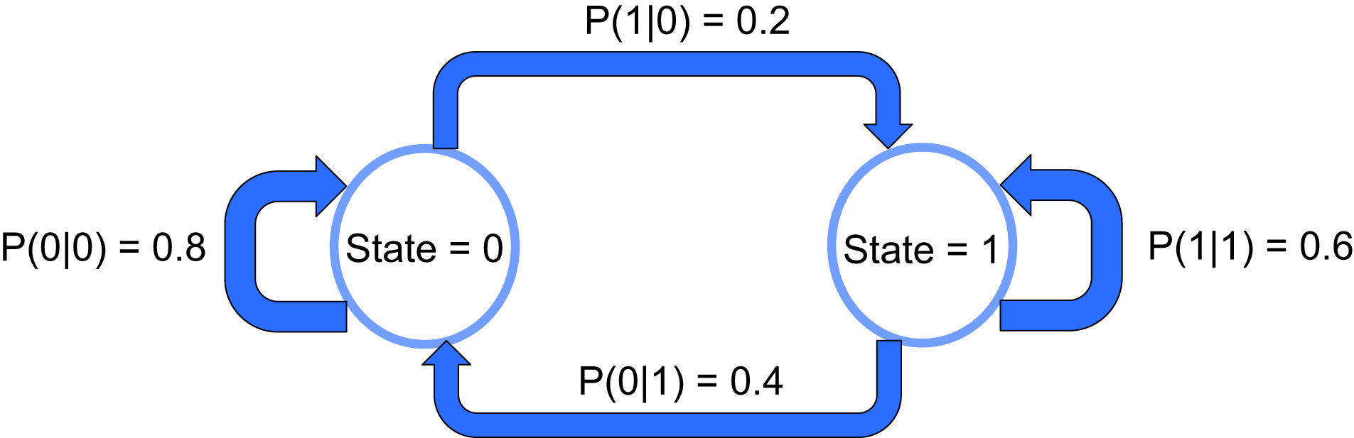
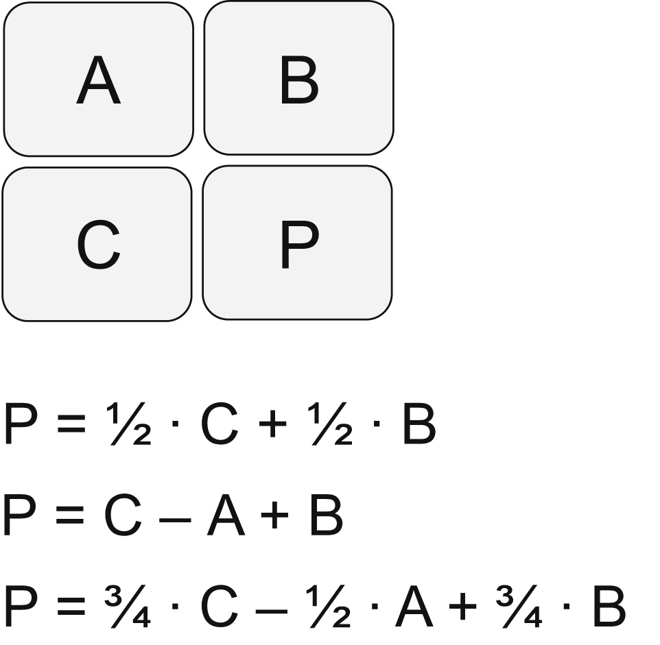
A first order binary Markov source can described in the diagram given in Fig. 24.4. The transition probabilities depend only on the current state.
In this case, the entropy can be found as the weighted sum of the conditional entropies corresponding to the transitional probabilities of the state diagram. The probability of a zero given the previous state is a 1 is described as P(0|1).
The probability of each state can be found by solving the probability equations:
Both methods a 0 can be output (meaning to arrive at state = 0 circle), either starting from state 0 or 1
Both methods a 1 can be output (meaning to arrive at state = 0 circle), either starting from state 0 or 1.
By definition P(0) + P(1) = 1.
From this, we can solve for P(0) and P(1)
P(0) = 2/3
P(1) = 1/3
Now we can solve for the entropy associated with each state circle.
For state 0 and state 1:
The entropy of the Markov source or system is then given by:
24.5. Predictive Coding
Finding the sequence “HAWAII” is a form of predictive coding. The probabilities of any Markov source, such as language, can be mapped in multiletter sequences with an associated probability. These in turn, can be encoded using Huffman coding methods, to produce a more efficient representation (fewer number of bits) of the outcome sequence.
This same idea can be applied to images. As we have previously seen, video images are built line by line, from top to bottom, and pixel by pixel, from left to right. Therefore, for a given pixel, the pixels above and to the left are available to help predict the next pixel. For our purposes here, let us assume an RGB video frame, with 8 bits per pixel and color. Each color can have a value from 0 to 255.
The value unknown pixel, for each color, can be predicted from the pixels immediately left, immediately above, and diagonally above. Three simple predictors are given below, in Fig. 24.5.
Now the entire frame could be iteratively predicted from just three initial pixels, but this is not likely to be a very good prediction. The usefulness of these predictors becomes apparent when used in conjunction with differential encoding.
24.6. Differential Encoding
Suppose instead we take the actual pixel value, and subtract the predicted pixel value. This is differential encoding, and this difference is used to represent the pixel value for that location. For example, to store a video frame, we would perform the differential encoding process, and store the results.
To restore the original video data for display, simply compute the predicted pixel value (using the previous pixel data) and then add to the stored differential encoded value. This is the original pixel data. (The three pixels on the upper left corner of the frame are stored in their original representation and are used to create the initial predicted pixel data during the restoration process).
All of this sounds unnecessarily complicated, so what is the purpose here? The reason to do this is that the differential encoder outputs are most likely to be much smaller values than the original pixel data, due to the correlation between nearby pixels. Since statistically, the differentially encoded data is just representing the errors of the predictor, this signal is likely to have the great majority of values concentrated around zero, or to have a very compact histogram. In contrast, the original pixel values are likely to span the entire color value space, and therefore are a high entropy data source with equal or uniform probability distribution.
What is happening with differential encoding is that we are actually sending less information than if the video frame was simply sent pixel by pixel across the whole frame. The entropy of the data stream has been reduced through the use of differential encoding, as the correlation between adjacent pixels has been largely eliminated. Since we have no information as to the type of video frames will be processed, the initial pixel values outcomes are assumed to be equally distributed, meaning each of the 256 possible values is equally with probability of 1/256, and entropy of 8 bits per pixel. The possible outcomes of the differential encoder tend be much more probable for small values (due to the correlation to nearby pixels) and much less likely for larger values. As we saw in our simple example above, when the probabilities are not evenly distributed, the entropy is lower. Lower entropy means less information. Therefore, on average, significantly less bits is required to represent the image, and the only cost is increased complexity due to the predictor and differential encoding computations.
Let us assume that averaged over a complete video frame, the probabilities work out as such:
Pixel color value Probability = 1/256 for values in range of 0–255
And that after differential encoder, the probability distribution comes out as:
Differential color Probability = 1/16 for value equal to 0
Differential color Probability = 1/25 for values in range of −8 to −1, 1 to 8
Differential color Probability = 1/400 for values in range of −32 to −9, 9 to 32
Differential color Probability = 1/5575 for values in range of −255 to −33, 33 to 255
Recall the entropy is defined as:
Entropy = prob (outcome1) · info (outcome1) + prob (outcome2) · info (outcome2) + … prob (outcomen) · info (outcomen)
with info of outcome = log2 (1/probability of that outcome)
In the first case, we have 256 outcomes, each of probability 1/256.
In the second case, we have 511 possible outcomes, with one of four probabilities. We will see that this has less entropy and can be represented in less than 8 bits of information.

24.7. Lossless Compression
The entropy has been significantly reduced through the use of the differential coder. Although this step function probability distribution is obviously contrived, typical entropy values for various differential encoders across actual video frame data tend to be in the range of 4–5 ½ bits. With use of Huffman coding or similar mapping of the values to bit codewords, the number of bits used to transmit each color plane pixel can be reduced to ∼5 bits compared to the original 8 bits. This has been achieved without any loss of video information, meaning the reconstructed video is identical to the original. This is known as lossless compression, as there is no loss of information in the compression (encoding) and decompression (decoding) processing.
Much higher degrees of compression are possible if we are willing to accept some level of video information loss, which can result in video quality degradation. This is known as lossy compression. Note that with lossy compression, each time the video is compressed and decompressed, some amount of information is lost, and there will be a resultant impact on video quality. The trick is to achieve high levels of compression, without noticeable video degradation.
One of the issues causes information loss in quantization, which we will examine next.
24.8. Quantization
Many of the techniques used in compression such as the DCT, Huffman coding, and predictive coding are fully reversible, with no loss in video quality. Quantization is often the principal area of compression where information is irretrievably lost, and the decoded video will suffer quality degradation. With care, this degradation can be made reasonably imperceptible to the viewer.
Quantization occurs when a signal with many or infinite number of values must be mapped into a finite set of values. In digital signal processing, signals are presented in binary numbers, with 2n possible values mapping into an n-bit representation.
For example, suppose we want to present the range −1 to +1 (well, almost +1) using an 8-bit fixed point number. With 2n or 256 possible values to map to across this range, the step size is 1/128, which works out to 0.0078125. Let us say the signal has an actual value of 0.5030. How closely can this value be presented? What if the signal is 1/10 the level of first sample, or 0.0503. And again, consider a signal with value 1/10 the level as the second sample, at 0.00503. Below is a table showing the closest representation just above and below each of these signal levels, and the error that will result in the 8-bit representation of the actual signal to sampled signal value.
| Signal Level | Closest 8 Bit Representation | Hexadecimal Value | Actual Error | Error as a Percent of Signal Level (%) |
| 0.50300 | 0.5000000 | 0x40 | 0.00300 | 0.596 |
| 0.50300 | 0.5078125 | 0x41 | −0.0048128 | 0.957 |
| 0.05030 | 0.0468750 | 0x06 | 0.003425 | 6.809 |
| 0.05030 | 0.0546875 | 0x07 | −0.0043875 | 8.722 |
| 0.00503 | 0.000000 | 0x00 | 0.00503 | 100 |
| 0.00503 | 0.0078125 | 0x01 | −0.0027825 | 55.32 |
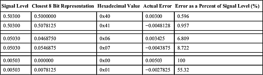
The actual error level remains more or less in the same range over the different signal ranges. This error level will fluctuate, depending on the exact signal value, but with our 8-bit signed example will always be less than 1/128, or 0.0087125. This fluctuating error signal will be seen as a form of noise or unwanted signal in the digital video processing. It can be modeled as an injection of noise when simulation an algorithm with unlimited numerical precision. It is called quantization noise.
When the signal level is fairly large for the allowable range (0.503 is close to one-half the maximum value) the percentage error is small—less than 1%. As the signal level gets smaller, the error percentage gets larger, as the table indicates.
What is happening is that the quantization noise is always present and is, on average, the same level (any noiselike signal will rise and fall randomly, so we usually concern ourselves with the average level). But as the input signal decreases in level, the quantization noise becomes more significant in a relative sense. Eventually, for very small input signal levels, the quantization noise can become so significant that it degrades the quality of whatever signal processing is to be performed. Think of it as like static on a car radio. As you get further from the radio station, the radio signal gets weaker, and eventually the static noise makes it difficult or unpleasant to listen to, even if you increase the volume.
So what can we do if our signal is sometimes strong (0.503, for example), and other times weak (0.00503, for example)? Another way of saying this is that the signal has a large dynamic range. The dynamic range describes the ratio between the largest and smallest value of the signal, in this case 100.
Suppose we exchange our 8-bit representation with 12-bit representation? Then our maximum range is still from −1 to +1, but our step size is now 1/2048, which works out to 0.000488. Let us make a 12-bit table similar to the 8-bit example.
| Signal Level | Closest 12 Bit Representation | Hexadecimal Value | Actual Error | Error as a Percent of Signal Level (%) |
| 0.50300 | 0.502930 | 0x406 | 0.000070 | 0.0139 |
| 0.50300 | 0.503418 | 0x407 | −0.000418 | 0.0831 |
| 0.05030 | 0.050293 | 0x067 | 0.000007 | 0.0140 |
| 0.05030 | 0.050781 | 0x068 | −0.000481 | 0.9568 |
| 0.00503 | 0.004883 | 0x00A | 0.000147 | 2.922 |
| 0.00503 | 0.005371 | 0x00B | −0.000341 | 6.779 |
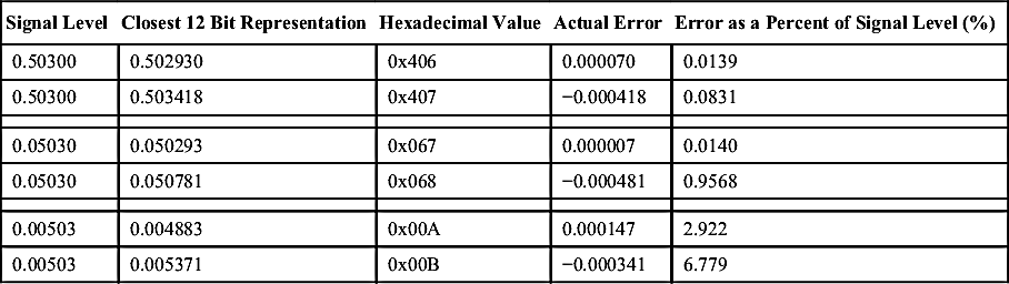
This is a significant difference. The actual error is always less than our step size, 1/2048. But the error as a percent of signal level is dramatically improved. This is what we usually care about in signal processing. Because of the much smaller step size of the 12-bit representation, the quantization noise is much less, allowing even small signals to be represented with very reasonable precision. Another way of describing this is to introduce the concept of signal-to-noise power ratio, or SNR. This describes the power of the largest signal compared to the background noise. This can be very easily seen on a frequency domain or spectral plot of a signal. There can be many sources of noise, but for now, we are only considering the quantization noise introduced by the digital representation of the video pixel values.
What we have just described is the uniform quantizer, where all the step sizes are equal. However, there are alternate quantizing mappings, where the step size varies across the signal amplitude. For example, a quantizer could be designed to give the same SNR across the signal range. This would require a small step size when the signal amplitude is small, and a larger step size as the signal increases in value. The idea is to provide a near constant quantization error as a percentage of the signal value. This type of quantizing is performed on the voice signals in the US telephone system, known as μ-law encoding.
Another possible quantization scheme could be to use a small step size for regions of the signal where there is a high probability of signal amplitude occurring, and larger step for regions where the signal has less likelihood of occurring.
However, in video signal processing, uniform quantizing is by far the most common. The reason is that often we are not encoding simply amplitude, representing small or large signals. In many cases, this could be color information, where the values map to various color intensities, rather than signal amplitude.
As far as trying to use likelihood of different values to optimize the quantizer, this assumes that this probability distribution of the video data is known. Alternatively, the uniform quantizer can be followed by some type of Huffman coding or differential encoding, which will optimize the signal representation for the minimum average number of bits.
Vector quantization is also commonly used. In the preceding discussion, a single set of values or signal is being quantized with a given bit representation. However, a collection of related signals can be quantized to a single representation using a given number of bits.
For example, assume the pixel is represented in RGB format, with 8 bits used for each color. This means that the color red can be represented in 28 or 256 different intensities.
Each pixel uses a total of 24 bits, for a total of 224, or about 16 million possible values. Intuitively, this seems excessive, can the human eye really distinguish that many colors? Instead, a vector quantizer might map this into a color table of 256 total colors, presenting 256 combinations of red, green, and blue combinations. This mapping results in requiring only 8 bits to present each pixel.
This seems like this might be reasonable, but the complexity is in trying to map the 16 million possible inputs to the allowed 256 representations, or color codewords. If done using a look up table, as memory of 16 million bytes would be required for this quantization, with each memory location containing one of the 256 color codewords. This is excessive, so some sort of mapping algorithm or computation is required to map these possible 16 million color combinations to the closest color codeword. As we are starting to see, most methods to compress video, or other data for that matter, come at the expense of increased complexity and increased computational rates.
24.9. Decibels
SNR is usually expressed in decibels (denoted dB), using a logarithmic scale. The SNR of a digital represented signal can be determined by the following equation:
Basically, for each additional bit of the signal representation, 6 dB of SNR is gained. Eight bit representation is capable of representing a signal with an SNR of about 48 dB, a 12 bits can do better at 72 dB, and 16 bits will give up to 96 dB. This only accounts for the effect of quantization noise; in practice there are other effects that could also will degrade SNR in a system.
There is another important point on decibels. These are very commonly used in many areas of digital signal processing subsystems. A decibel is simply a signal power ratio, similar to percentage. But because of the extremely high ratios commonly used (a billion is not uncommon), it is convenient to express this logarithmically. The logarithmic expression also allow chains of circuits or signal processing operations each with its own ratio (say of output power to input power) to simply be added up to find the final ratio.
Where people commonly get confused is in differentiating between signal levels or amplitude (voltage if an analog circuit) and signal power. Power measurements are virtual in the digital world, but can be directly measured in analog circuits in which video systems interface with, such as the RF amplifiers and analog signal levels for circuits in head-end cable systems, or video satellite transmission.
There are two definitions of dB commonly used.
The designations of “signal 1” and “signal 2” depend on the situation. For example, with an RF power amplifier, the dB of gain will be the 10 log (output power/input power). For digital, the dB of SNR will be the 20 log (maximum input signal/quantization noise signal level).
The use of dB can refer to many different ratios in video system designs. But it is easy to get confused whether to use to multiplicative factor of 10 or 20, without understanding the reasoning behind this.
Voltage squared is proportional to power. If a given voltage is doubled in a circuit, it requires four times as much power. This goes back to a basic Ohm's law equation.
In many analog circuits, signal power is used, because that is what the lab instruments work with, and while different systems may use different resistance levels, power is universal (however, 50 Ω is the most common standard in most analog systems).
The important point is that since voltage is squared, this effect needs to be taken into account in the computation of logarithmic decibel relation. Remember,  . Hence, the multiply factor of “2” is required for voltage ratios, changing the “10” to a “20”.
In the digital world, the concept of resistance and power do not exist. A given signal has specific amplitude, expressed in a digital numerical system (such as signed fractional or integer, for example).
Understanding dB increases using the two measurement methods is important. Let us look at doubling of the amplitude ratio and doubling of the power ratio.
This is why shifting a digital signal left 1 bit (multiply by 2) will cause a 6 dB signal power increase, and why so often the term 6 dB/bit is used in conjunction with ADCs, DACs, or digital systems in general.
By the same reasoning, doubling in power to an RF engineer means a 3 dB increase. This will also impact the entire system. Coding gain, as used with error-correcting code methods, is based on power. All signals at antenna interfaces are defined in terms of power, and the decibels used will be power ratios.
In both systems, ratio of equal power or voltage is 0 dB. For example, a unity gain amplifier has a gain of 0 dB.
A loss would be expressed as a negative dB. For example a circuit whose output is equal to ½ the input power.
..................Content has been hidden....................
You can't read the all page of ebook, please click here login for view all page.