
Chapter 15. Action Planning
This chapter gives a general introduction to search problems for optimal and suboptimal action planning, including state space search for numerical and temporal planning domains. It also considers plan constraints and soft goals.
Keywords: action planning, optimal planning, Graphplan, Satplan, planning pattern database, causal graph, metric planning, temporal planning, derived predicate, timed initial literal, state trajectory constraint, preference constraint
In domain-independent action planning, a running system must be able to find plans and exploit search knowledge fully automatically. In this chapter we concentrate on deterministic planning (each action application produces exactly one successor) with no uncertainty in the environment and no observation to infer otherwise inaccessible state variables. The input of a planning problem consists of a set of state variables, an initial state in the form of value assignments to the variables, a goal (condition), and a set of actions. A plan is a sequence (or schedule) of actions that eventually maps the initial state into one that satisfies the goal.
The problem domain description language (PDDL) allows flexible specifications of domain models and problem instances. Starting from problems described in Strips notation (as introduced in Ch. 1), PDDL has grown to an enormous expressive power, including large fragments of first-order logic to combine propositional expressions, numerical state variables to feature the handling of real-valued quantities, and constraints to impose additional restrictions for the set of valid plans. Metric planning introduces planning with costs, and temporal planning covers action duration. The agreed standard for PDDL encompasses the following hierarchy of expressiveness.
Level 1: Propositional Planning. This level includes all sorts of propositional description languages. It unifies Strips-type planning with the abstract description language (ADL). ADL allows typed domain objects and any bounded quantification over these. ADL also includes negated and disjunctive preconditions, and conditional effects. While the former two language extensions can be easily compiled away (by introducing negated predicates and by splitting the actions), the latter ones are essential in the sense that their compilation may induce an exponential increase in the problem specification. Propositional planning is decidable, but PSPACE-hard.
Level 2: Metric Planning. This level introduces numerical state variables, so-called fluents, and an objective function to be optimized (the domain metric ) that judges plan quality. Instead of Boolean values to be associated with each grounded atom, the language extension enables the processing of continuous quantities, an important requirement for modeling many real-world domains. This growing expressiveness comes at a high price. Metric planning is undecidable even for very restricted problem classes (a decision problem is undecidable if is impossible to construct one computable function that always terminates and leads to a correct answer). This, however, does not mean that metric planners cannot succeed in finding plans for concrete problem instances.
Level 3: Temporal Planning. This level introduces duration, which denotes action execution time. The duration can be a constant quantity or a numerical expression dependent on the current assignment to state variables. Two different semantics have been proposed. In the PDDL semantics each temporal action is divided into an initial, an invariant, and a final happening. Many temporal planners, however, assume the simpler black-box semantics. The common task is to find a temporal plan, i.e., a set of actions together with their starting times. This plan is either sequential (simulating additive action costs) or parallel (allowing the concurrent execution of actions). The minimal execution time of such a temporal plan is its makespan, and can be included as one objective in the domain metric.
More and more features have been attached to this hierarchy. Domain axioms in the form of derived predicates introduce inference rules, and timed initial facts allow action execution windows and deadlines to be specified. Newer developments of PDDL focus on temporal and preference constraints for plans. Higher levels support continuous processes and triggered events.
The results of the biennial international planning competitions (started in 1998) show that planners keep aligned with the language extensions, while preserving good performances in finding and optimizing plans. Besides algorithmic contributions, the achievements also refer to the fact that computers have increased in their processing power and memory resources.
As a consequence, modern action planning is apparently suited to provide prototypical solutions to specific problems. In fact, action planning becomes more and more application oriented. To indicate the range and flavor of applicability of modern action planning, we list some examples that have been proposed as benchmarks in the context of international planning competitions.
Airport The task is to control the ground traffic on an airport, assigning travel routes and times to the airplanes, so that the outbound traffic has taken off and the inbound traffic is parked. The main problem constraint is to ensure the safety of the airplanes. The aim is to minimize the total travel time of all airplanes.
Pipesworld The task is to control the flow of different and possibly conflicting oil derivatives through a pipeline network, so that certain product amounts are transported to their destinations. Pipeline networks are modeled as graphs consisting of areas (nodes) and pipes (edges), where the pipes can differ in length.
Promela The task is to validate state properties in systems of communicating processes. In particular, deadlock states shall be detected, i.e., states where none of the processes can apply a transition. For example, a process may be blocked when trying to read data from an empty communication channel.
Power Supply Restoration The task is to reconfigure a faulty electricity network, so that a maximum of nonfaulty lines is supplied. There is uncertainty about the status of the network, and various numerical parameters must be optimized.
Satellite The domain is inspired from a NASA application, where satellites have to take images of spatial phenomena and send them back to Earth. In an extended setting, timeframes for sending messages to the ground stations are imposed.
Rovers The domain (also inspired from a NASA application) models the problem of planning for a group of planetary rovers to explore the planet they are on, for example, by taking pictures and samples from interesting objects.
Storage The domain involves spatial reasoning and is about moving a certain number of crates from some containers to some depots by hoists. Inside a depot, each hoist can move according to a specified spatial map connecting different areas of the depot.
Traveling Purchase Problem A generalization of the TSP. We have a set of products and a set of markets. Each market is provided with a limited amount of each product at a known price. The task is to find a subset of the markets such that a given demand of each product can be purchased, minimizing the routing and the purchasing costs.
Openstack A manufacturer has a number of orders, each for a combination of different products, and can make one product at a time only. The total required quantity of each product is made at the same time. From the time that the first product (included in an order) is made to the time that all products (included in the order) have been made, the order is said to be open. During this time it requires a stack. The problem is to order the production of the different products, so that the maximum number of stacks that are in use simultaneously is minimized.
Trucks Essentially, this is a logistics domain about moving packages between locations by trucks under certain constraints. The loading space of each truck is organized by areas: a package can be loaded onto an area of a truck only if the areas between the area under consideration and the truck door are free. Moreover, some packages must be delivered within given deadlines.
Settlers The task is to build up an infrastructure in an unsettled area, involving the building of housing, railway tracks, sawmills, etc. The distinguishing feature of the domain is that most of the domain semantics are encoded with numeric variables.
UMTS The task is the optimization of the call setup for mobile applications. A refined schedule for the setup is needed to order and accelerate the execution of the application modules that are invoked during the call setup.
Probably the most important contribution to cope with the intrinsic difficulty of domain-independent planning was the development of search guidance in the form of generic heuristics. In the following, we introduce designs for planning heuristics and show how to tackle more expressive planning formalisms, like metric and temporal planning, as well as planning with constraints.
15.1. Optimal Planning
Optimal planners compute the best possible plan. They minimize the number of (sequential or parallel) plan steps or optimize the plan with respect to the plan metric. There are many different proposals for optimal planning, ranging from plan graph encoding, satisfiability solving, integer programming to constraint satisfaction, just to name a few. Many modern approaches consider heuristic search planning based on admissible estimates.
We first introduce optimal planning via layered planning graphs and via satisfiability planning. Next, admissible heuristics are devised that are based on dynamic programming or on pattern databases.
15.1.1. Graphplan
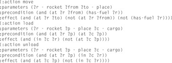
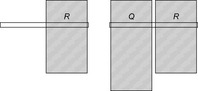
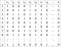
Graphplan is a parallel-optimal planner for propositional planning problems. The rough working of the Graphplan algorithm is the following. First, the parametric input is grounded. Starting with a planning graph, which only consists of the initial state in the first layer, the graph is incrementally constructed. In one stage of the algorithm, the planning graph is extended with one action and one propositional layer followed by a graph extraction phase. If this search terminates with no solution, the plan horizon is extended with one additional layer. As an example, consider the Rocket domain for transporting cargo in space (see Fig. 15.1). The layered planning graph is shown in Table 15.1.
In the forward phase the next action layer is determined as follows. For each action and each instantiation of it, a node is inserted, provided that no two preconditions are marked as mutually exclusive (mutex ). Two propositions a and b are marked mutex, if all options to generate a are exclusive to all options to generate b. Additionally, so-called noop actions are included that merely propagate existing propositions to the next layer. Next, the actions are tested for exclusiveness and for each action a list of all other actions is recorded, for which they are exclusive. To generate the next propositional layer, the add-effects are inserted and taken as the input for the next stage.
A fixpoint is reached when the set of propositions no longer changes. As one subtle problem, this test for termination is not sufficient. Consider a goal in Blocksworld given by (on a b), (on b c), and (on c a). Every two conditions are satisfiable but not all three all together. Thus, the forward phase terminates if the set of propositions and the goal set in the previous stage have not changed.
It is not difficult to see that the size of the planning graph is polynomial in the number n of objects, the number m of action schemas, the number p of propositions in the initial state, the length l of the longest add-list, and the number of layers in the planning graph. Let k be the largest number of action parameters. The number of instantiated effects is bounded by  . Therefore, the maximal number of nodes in every propositional layer is bounded by
  . Since every action schema can be instantiated in at most
  different ways, the maximal number of nodes in each action layer is bounded by
  .
.
In the generated planning graph, Graphplan constructs a valid plan, chaining backward from the set of goals. In contrast to most other planners, this processing works layer by layer to take care of preserving the mutex relations. For a given time step t, Graphplan tries to extract all possible actions (including noops) from time step t − 1, which has the current subgoal as add-effects. The preconditions for these actions build the subgoals to be satisfied in time step t − 1 to satisfy the chosen subgoal at time step t. If the set of subgoals is not solvable, Graphplan chooses a different set of actions, and recurs until all subgoals are satisfied or all possible combinations have been exhausted. In the latter case, no plan (with respect to the imposed depth threshold) exists, as it can be shown that Graphplan terminates with failure if and only if there is no solution to the current planning problem. The complexity of the backward phase is exponential (and has to be unless PSPACE = P). By its layered construction, Graphplan constructs a plan that has the smallest number of parallel plan steps.
15.1.2. Satplan
To cast a fully instantiated action planning task as a satisfiability problem we assign to each proposition a time stamp denoting when it is valid. As an example, for the initial state and goal condition of a sample Blocksworld instance, we may have generated the formula Further formulas express action execution. They include action effects, such as
 and noop clauses for propositions to persist. To express that no action with unsatisfied precondition is executed, we may introduce rules, in which additional action literals imply their preconditions, such as
 Effects are dealt with analogously. Moreover, (for sequential plans) we have to express that at one point in time only one action can be executed. We have
 Finally, for a given step threshold N we require that at every step i < N at least one action has to be executed; for all i < N we require
The only model of this planning problem is (move a b t 1), (move b t a 2). Satplan is a combination of a planning problem encoding and an SAT solver. The planner's performance participates in the development of more and more efficient SAT solvers.
Extensions of Satplan to parallel planning encode the planning graph and the mutexes of Graphplan. For this approach, Satplan does not find the plan with the minimal total number of steps, but the one with the minimal number of parallel steps.
15.1.3. Dynamic Programming
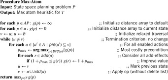
One of the first estimates for heuristic search planning is the max-atom heuristic. It is an approximation of the optimal cost for solving a relaxed problem in which the delete lists are ignored. An illustration is provided in Figure 15.2 (left).
The heuristic is based on dynamic programming. Consider a propositional and grounded propositional planning problem  (see Ch. 1) with planning states u and v, and propositions p and q. Value
  is the sum of the approximations g(u, p), to reach p from u, where
 is a fixpoint equation. The recursion starts with g(u, p) = 0, for p ∈ u, and g(u, p) = ∞, otherwise. The values of g are computed iteratively, until the values no longer change. The costs g(u, C) for the set C is computed as
  . In fact, the cost of achieving all the propositions in a set can be computed as either a sum (if sequentiality is assumed) or as a max (if parallelism is assumed instead). The max-atom heuristic chooses the maximum of the cost values with
  . The pseudo code is shown in Algorithm 15.1. This heuristic is consistent, since by taking the maximum cost values, the heuristic on an edge can decrease by at most 1.
As the heuristic determines the backward distance of atoms with respect to the initial state, the previous definition of the heuristic is of use only for backward or regression search. However, it is not difficult to implement a variant that is applicable to forward or progression search, too.
The max-atom heuristic has been extended to max-atom-pair to include larger atom sets, which enlarges the extracted information (without losing admissibility) by approximating the costs of atom pairs: where p & q denotes that p and q are both contained in the add list of the action, and where p|q denotes that p is contained in the add list and q is neither contained in the add list nor in the delete list. If all goal distances are precomputed, then these distances can be retrieved from a table, yielding a fast heuristic.
The extension to hm with atom sets of  elements has to be expressed with the following recursion:
 where R(C) denotes all pairs (D, O) that contain
  ,
,  , and
, and  . It is rarely used in practice.
It has been argued that the layered arrangement of propositions in Graphplan can be interpreted as a special case of a search with h2.
15.1.4. Planning Pattern Databases
In the following, we study how to apply pattern databases (see Ch. 4) to action planning. For a fixed state vector (in the form of a set of instantiated predicates) we provide a general abstraction function. The ultimate goal is to create admissible heuristics for planning problems fully automatically.
Planning patterns omit propositions from the planning space. Therefore, in an abstract planning problem with regard to a set  , a domain abstraction is induced by
  . (Later on we will discuss how R can be selected automatically.) The interpretation of ϕ is that all Boolean variables for propositions not in R are mapped to don't care. An abstract planning problem
 of a propositional planning problem (S, A, s, T) with respect to a set of propositional atoms R is defined by
  ,
,  ,
,  ,
,  , where a|R for
  is given as
  . An illustration is provided in Figure 15.2 (right).
This means that abstract actions are derived from concrete ones by intersecting their precondition, add, and delete lists with the subset of predicates in the abstraction. Restriction of actions in the concrete space may yield noop actions in the abstract planning problem, which are discarded from the action set A|R.
A planning pattern database with respect to a set of propositions R and a propositional planning problem  is a collection of pairs (d, v) with
  and d being the shortest distance to the abstract goal. Restriction |R is solution preserving; that is, for any sequential plan π for the propositional planning problem P there exists a plan πR for the abstraction
  . Moreover, an optimal abstract plan for P|R is shorter than or equal to an optimal plan for P. Strict inequality holds if some abstract actions are noops, or if there are even shorter paths in the abstract space. We can also prove consistency of pattern database heuristics as follows. For each action a that maps u to v in the concrete space, we have
  . By the triangular inequality of shortest paths, the abstract goal distance for ϕ(v) plus one is larger than or equal to the abstract goal distance ϕ(u).
Figure 15.3 illustrates a standard (left) and multiple pattern database (right) showing that different abstractions may refer to different parts of the state vector.
Encoding
Propositional encodings are not necessarily the best state space representations for solving propositional planning problems. A multivalued variable encoding is often better. It transforms a propositional planning task into an SAS+ planning problem, which is defined as a quintuple  , with
  being a set of state variables of states in S(each
  has finite-domain Dv), A being a set of actions given by a pair (P, E) for preconditions and effects, and s and T being the initial and goal state s, respectively, in the form of a partial assignment. A partial assignment for X is a function s over X, such that
  , if s(v) is defined.
The process of finding a suitable multivalued variable encoding is illustrated with a simple planning problem, where a truck is supposed to deliver a package from Los Angeles to San Francisco. The initial state is defined by the atoms (ispackage package), (istruck truck), (location los-angeles), (location san-francisco), (at package los-angeles), and (at truck los-angeles). Goal states have to satisfy the condition (at package san-francisco). The domain provides three action schemas named load to load a truck with a certain package at a certain location, the inverse operation unload, and drive to move a truck from one location to another.
The first preprocessing step will detect that only the at (denoting the presence of a given truck or package at a certain location) and in predicates (denoting that a package is loaded in a certain truck) change over time and need to be encoded. The labeling predicates ispackage, istruck, location are not affected by any action and thus do not need to be specified in a state encoding.
In a next step, some mutual exclusion constraints are discovered. In our case, we will detect that a given object will always be at or in at most one other object, so propositions such as (at package los-angeles) and (in package truck) are mutually exclusive. This result is complemented by fact space exploration: Ignoring negative (delete) effects of actions, we exhaustively enumerate all propositions that can be satisfied by any legal sequence of actions applied to the initial state, thus ruling out illegal propositions, such as (in los-angeles package), (at package package), or (in truck san-francisco). Now all the information that is needed to devise an efficient state encoding schema for this particular problem is at the planner's hands. We discover that three multivalued variables are needed. The first one is required for encoding the current city of the truck and the other two variables are required to encode the status of the package.
Using the multivalued variable encoding the number of possible planning states shrinks drastically, whereas the number of reachable planning states remains unchanged. As another consequence, the multivalued variable encoding provides better predictions to the expected sizes of the abstract planning spaces.
Multiple Pattern Databases
As abstract planning problems are defined by a selection R of atoms there are several different candidates for a pattern database. This remains true when projecting multivalued variables.
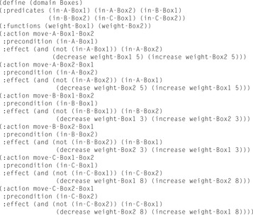
We exemplify our considerations in Blocksworld. The domain is specified with the four action schemas pick-up, put-down, stack, and unstack, and the propositions on, ontable, handempty, and clear. The example problem contains four blocks a, b, c, and d used for grounding. For example, (pick–up a) is defined as the precondition list {(clear a), (ontable a), (handempty)}, the add list {(holding a)}, and the delete list {(ontable a), (clear a), (handempty)}. The goal of the instance is {(on d c), (on c a), (on a b)} and the initial state is given by {(clear b), (ontable d), (on b c), (on c a), (on a d)}.
One possible multivalued variable encoding for the domain, consisting of groups of mutually exclusive propositions, which has been automatically inferred by a static analyzer (as explained earlier) has nine variable domains: Dv1 = {(on c a), (on d a), (on b a), (clear a), (holding a)} (for the blocks on top of a); Dv2 = {(on a c), (on d c), (on b c), (clear c), (holding c)} (for the blocks on top of c); Dv3 = {(on a d), (on c d), (on b d), (clear d), (holding d)} (for the blocks on top of d); Dv4 = {(on a b), (on c b), (on d b), (clear b), (holding b)} (for the blocks on top of b); Dv5 = {(ontable a), none} (is block a bottom-most in tower); Dv6 = {(ontable c), none} (is block c bottom-most in tower); Dv7 = {(ontable d), none} (is block d bottom-most in tower); Dv8 = {(ontable b), none} (is block b bottom-most in tower); and Dv9 = {(handempty), none} (for the gripper). Each state can be expressed by selecting one proposition for each variable and none refers to the absence of all other propositions in the group.
We may select variables with even index to define the abstraction  and variables with odd index to define the abstraction
  . The resulting planning databases are depicted in Table 15.2. Note that there are only three atoms present in the goal state so that one of the pattern databases only contains patterns of length one. Abstraction
  corresponds to v1 and
  corresponds to the union of v2 and v4.
To construct an explicit-state pattern database, one can use a hash table for storing the goal distance for each abstract state. In contrast, symbolic planning pattern databases are planning pattern databases that have been constructed with BDD exploration for latter use either in symbolic or explicit heuristic search. Each search layer is represented by a BDD. In planning practice, a better scaling seems to favor symbolic pattern database construction.
Pattern Addressing
To store the pattern databases, large hash tables are required. The estimate of a state is then a mere hash lookup (one for each pattern database). To improve efficiency of the lookup, it is not difficult to devise an incremental hashing scheme.
First, we assume a propositional encoding. For  we select
  as the hash function with prime q denoting the size of the hash table. The hash value of
  can be incrementally calculated as
 Of course, hashing induces a (clearly bounded) number of collisions that have to be resolved by using one of the techniques presented in Chapter 3.
Since  can be precomputed for all
  , we have an incremental running time to compute the hash address that is of order
  , which is almost constant for most propositional planning problems (see Ch. 1). For constant time complexity we store
  together with each action a. Either complexity is small, when compared with the size of the planning state.
It is not difficult to extend incremental hash addressing to multivalued variables. According to the partition into variables, a hash function is defined as follows. Let  be the selected variables in the current abstraction and
  . Furthermore, let
  and
and  be, respectively, the variable index and the position of proposition p in its variable group. Then, the hash value of state u is
 The incremental computation of h(v) for
  is immediate.
Automated Pattern Selection
Even in our simple example planning problem, the number of variables and the sizes of the generated pattern databases for  and
and  differ considerably. Since we perform a complete exploration for pattern database construction, time and space resources may become exhausted. Therefore, an automatic way to find a balanced partition with regard to a given memory limit is required. Instead of imposing a bound on the total size for all pattern databases altogether, we impose a threshold for the sizes of the individual pattern databases, which has to be adapted to a given infrastructure.
As shown in Chapter 4, one option for pattern selection is Pattern Packing: According to the domain sizes of the variables, it finds a selection of pattern databases so that their combined sizes do not exceed the given threshold.
In the following, we consider genetic algorithms for improved pattern selection, where pattern genes denote which variable appears in which pattern. Pattern genes have a two-dimensional layout (see Fig. 15.4). It is recommended to initialize the genes with Pattern Packing. To avoid that all genes of the initial population are identical, the variable ordering for Pattern Packing can be randomized.
 |
| Figure 15.4 |
A pattern mutation flips bits with respect to a small probability. This allows us to add or delete variables in patterns. We extended the mutation operator to enable insertion and removal of entire patterns. Using selection, an enlarged population produced by recombination is truncated to its original size, based on their fitness. The (normalized) fitness for the population is interpreted as a distribution function for selecting the next population. Consequently, genes with higher fitness are chosen with higher probability.
The higher the distance-to-goal values in abstract space, the better the quality of the corresponding database in accelerating the search in the concrete search space. As a consequence, we compute the mean heuristic value for each of the databases and superimpose it over a pattern partitioning. If  ,
,  is the i th pattern database and
  its maximal h-value, then the fitness for gene g is
 or
or where the operator depends on the disjointness of the multiple pattern databases.
15.2. Suboptimal Planning
For suboptimal planning we first introduce the causal graph heuristic based on the multivalued variable encoding. Then we consider extensions of the relaxed planning heuristic (as introduced in Ch. 1) to metric and temporal planning domains.
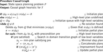
15.2.1. Causal Graphs
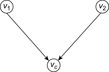
There are two main problems of the relaxed planning heuristic (see Ch. 1). First, unsolvable problems can become solvable, and, second, the distance approximations may become weak. Take, for example, the two Logistics problems in Figure 15.5. In both cases, we have to deliver a package to its destination (indicated with a shaded arrow) using some trucks (initially located at the shaded nodes). In the first case (illustrated on the left) a relaxed plan exists, but the concrete planning problem (assuming traveling constraints induced by the edges) is actually unsolvable.
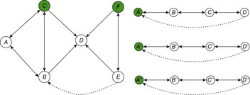
In the second case (illustrated on the top right) a concrete plan exists. It requires moving the truck to pick up the package and return it to its home. The relaxed planning heuristic returns a plan that is about half as good. If we scale the problem as indicated to the lower part of the figure, heuristic search planners based on the relaxed planning heuristic quickly fail.
The causal graph analysis is based on the following multivalued variable encoding ,
,  ,
,  ,
,  ,
,  ,
,  ,
,  , …,
, …, 
 },
},  , and
, and  .
.
The causal graph of an SAS+ planning problem P with variable set X is a directed graph  , where
  if and only if
  and there is an action
  , such that
  is defined and either
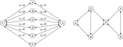
  or eff (u) is defined. This implies that an edge is drawn from one variable to another if the change of the second variable is dependent on the current assignment of the first variable. The causal graph of the first example (Fig. 15.5, left) is shown in Figure 15.6. These (in practice acyclic) graphs are divided into high-level (vc) and low-level variables (v1 and v2).
 |
| Figure 15.6 |
Given an SAS+ planning problem with  , the domain transition graph Gv is a directed labeled graph with node set Dv. Being a projection of the original state space it contains an edge
  if there is an action
  with
with  (or
(or  undefined) and
  . The edge is labeled by
  . The domain transition graph for the example problem is shown in Figure 15.7.
 |
| Figure 15.7 |
Plan existence in SAS+ planning problems is provably hard. Hence, depending on the structure of the domain transition graph(s), a heuristic search planning algorithm approximates the original problem. The approximation, measured in the number of executed plan steps, is used as a (nonadmissible) heuristic to guide the search in the concrete planning space.
Distances are measured between different value assignments to variables. The (minimal) cost  to change the assignment of v from d to
  is computed as follows. If v has no causal predecessor,
  is the shortest path distance from d to
  in the domain transition graph, or
  , if no such path exists. Let Xv be the set of variables that have v and all immediate predecessors of v in the causal graph of P. Let Pv be the subproblem induced by Xv with the initial value of v being d and the goal value of v being
  . Furthermore, let
  , where π is the shortest plan computed by the approximation algorithm (see later). The costs of the low-level variables are the shortest path costs in the domain transition graph, and 1 for the high-level variables. Finally, we define the heuristic estimate h(u) of the multivalued planning state u as
The approximation algorithm uses a queue for each high-level variable. It has polynomial running time but there are solvable instances for which no solution is obtained. Based on a queue Q it roughly works as shown in Algorithm 15.2.
Applied to an example (see Fig. 15.5, right), Q initially contains the elements  . The stages of the algorithms are as follows. First, we remove D from the queue, such that
  . Choosing (pickup D) yields
  (move A B), (move B C), (move C D), (pickup D)). Next, we remove t from the queue, such that
  . Choosing (drop A) yields
  (move A B), (move B C), (move C D), (pickup D), (move D C), (move C B), (move B A), (drop A)). Choosing (drop B), (drop C), (drop D) produces similar but shorter plans. Afterward, we remove C from the queue, such that
  yields no improvement. Subsequently, B is removed from the queue, such that
  yields no improvement. Lastly, A is removed from the queue and the algorithm terminates and returns
  .
.
15.2.2. Metric Planning
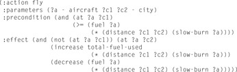
Metric planning involves reasoning about continuous state variables and arithmetic expressions. An example for an according PDDL action is shown in Figure 15.8.
 |
| Figure 15.8 |
Many existing planners terminate with the first solution they find. Optimization in metric planning, however, calls for improved exploration algorithms.
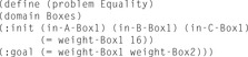
The state space of a metric planning instance is the set of assignments to the state variables with valid values. The logical state space is the result of projecting the state space to the components that are responsible for representing predicates. Analogously, the numerical state space is the result of projecting the state space to the components that represent functions. Figure 15.10 shows an instantiated problem, which refers to the domain Boxes shown in Figure 15.9.
 |
| Figure 15.10 |
In metric planning problems, preconditions and goals are of the form  , where
  and
and  are arithmetic expressions over the sets of variables and operators
  and where
  is selected from
  , ≤, >, <,
  . Assignments are of the form
  with head v and exp being an arithmetic expression (possibly including v). Additionally, a domain metric can be specified which has to be minimized or maximized over the end states of all valid plans. Costs in the domain metric refer to assignments to the numerical state variables.
Metric planning is an essential language extension. Since we can encode the working of random access machines in real numbers, even the decision problem, whether or not a plan exists, is undecidable. The undecidability result show that in general we cannot prove that a problem obeys no solution. However, if there is one, we may be able to find it. Moreover, as metric planning problems may span infinite state spaces, heuristics to guide the search process are even more important than for finite-domain planning problems. For example, we know that A* is complete even on infinite graphs, given that the cumulated costs of every infinite path is unbounded.
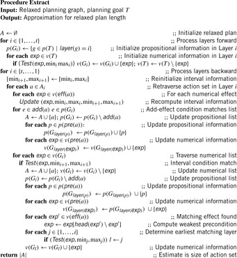
Heuristic Estimate
The metric version of the propositional relaxed planning heuristic analyzes an extended layered planning graph, where each fact layer includes the encountered propositional atoms and numerical variables. The forward construction of the planning graph iteratively applies actions until all goals are satisfied. In the backward greedy plan extraction phase the atoms and variables in the preconditions are included in a pending queue as still to be processed. In contrast to the propositional relaxed planning heuristic, multiple applications of actions have to be granted, otherwise the inference of a numeric goal, say 100, by a single increment operator does not approximate the hundred steps needed. For this case, numeric conditions in the pending queue need to be propagated backward through a selected action.
As a consequence, we have to determine the weakest precondition using the Hoare calculus, a well-known concept to determine the partial correctness of computer programs. Its assignment rule states that  , where x is a variable, p is a postcondition, and
  is the substitution of t in x. As an example consider the assignment
  with postcondition p given as
  . To find the weakest precondition we take
  , such that
  evaluates to
  and
and  . For the application in relaxed metric planning, assume that an assignment of the form
  is subject to a postcondition
  . The weakest precondition of it is established by substituting the occurrence of h in
  with exp. In a tree representation this corresponds to insert exp at all leaves that correspond to h as subtrees in
  . Usually, a simplification algorithm refines the resulting representation of
  .
.
In Algorithm 15.3 we illustrate the plan construction process in pseudo code. For each layer t in the relaxed planning graph a set of active propositional and numerical constraints is determined. We use p(⋅) to select valid propositions and  to select the variables. To determine the set of applicable actions At, we assume to have implemented a recursive procedure Test. The input of this procedure is a numerical expression and a set of intervals
  ,
,  that describe lower and upper assignment bounds for each variable vi. The output is a Boolean value that indicates whether the current assignment fits into the corresponding bounds. We also assume a recursive implementation forUpdate to adjust the bounds mint and maxt to mint+1 and maxt+1 according to a given expression exp.
For the extraction process as shown in Algorithm 15.4 we first search for the minimal layer in which the chosen condition is satisfied. The propositional and numerical pending queues in layer i are denoted by  and
and  . These pending queues represent the conditions for the particular layer that have to be achieved while constructing the relaxed plan. Although the initialization for the propositional part given the compound goal condition is rather simple (see with the relaxed planning heuristic in Ch. 1), for the initialization of the numerical condition queue the variable intervals
  for an increasing layer i are utilized to test the earliest satisfaction of the goal condition.

Now the constructed planning graph is traversed backward, layer by layer. To find the set of active actions, we reuse the set Ai and recompute the vectors  and
and  as determined in the forward phase. We continue until either an add-effect of an action in
  is detected or the numerical conditions of an effect become satisfied. In both cases we add the corresponding action to the relaxed plan and propagate the propositional preconditions of the chosen action to the layer in the relaxed planning graph, where they are satisfied for the first time as still to be processed.
The remaining code fragment (starting with for each considers how numeric postconditions are propagates by themselves. For the ease of presentation we restrict to ordinary assignments. After an assignment is chosen, we determine the weakest precondition for the expression as described earlier. It is also added to the pending queue of the shallowed level, in which it is satisfied. This layer can easily be determined by iteratively calling Test for the layers
  .
.
For example, if we have a postcondition of  and an assignment
  in one of the action effects, the weakest precondition to be progressed (according to Hoare's assignment rule) is
  , which is equivalent to
  . The latest layer in which this condition is satisfied might be the one where we started. So if we have the interval
  for v in the current layer i, and [0, 75] in the previous layer i − 1, we include the action in the relaxed plan 25 times until v ≤ 75, at which time the condition is included in the pending queue of layer i − 1.
15.2.3. Temporal Planning
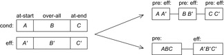
Temporal planning domains include temporal modifiers at start, over all, and at end, where label at start denotes the preconditions and effects at invocation time of the action, over all refers to an invariance condition that must hold, and at end refers to the finalization conditions and consequences of the action. An example for a PDDL action with numbers and durations is shown in Figure 15.11.

Temporal Model
There are mainly two different options to translate the temporal information back to metric planning problems with preconditions and effects. In the first case, the compound action is split into three smaller parts: one for action invocation, one for invariance maintenance, and one for action termination. This is the suggested semantic of PDDL2.1 (see Fig. 15.12, top right). As expected, there are no effects in the invariance pattern, so that  . Moreover, for benchmarks it is uncommon that new effects in at-start are preconditioned for termination control or invariance maintenance, such that
  . In these problems, a simpler model can be applied, using only one untimed variant for each temporal action (see Fig. 15.12, bottom right). For most planning benchmarks there are no deficiencies by assuming this temporal model, in which each action starts immediately after a previous one has terminated.
 |
| Figure 15.12 |
These black-box semantics allow the modifiers to be dropped since conditions are checked at the beginning and effects are checked at the end. The instantiation of a timed version of the Boxes domain is provided in Figure 15.13.
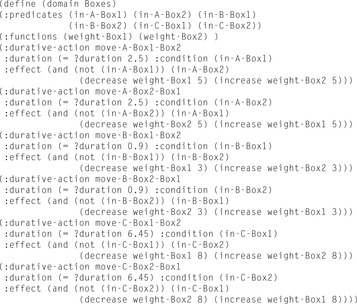
Action Dependency
The purposes of defining action dependency are twofold. First, at least one execution order of two independent actions can be pruned from the search tree and, more importantly, it is possible to compute optimal schedules of sequential plans with respect to the generated action sequence and its causal structure. If all actions are dependent (or void with respect to the optimizer function), the problem is inherently sequential and no schedule leads to any improvement.
Two grounded actions are dependent if one of the following conditions holds:
1. The propositional precondition set of one action has a nonempty intersection with the add or the delete lists of the other one (propositional conflict).
2. The head of a numerical modifier of one action is contained in some condition of the other one. Intuitively, an action modifies variables that appear in the condition of the other (direct numerical conflict).
3. The head of the numerical modifier of one action is contained in the formula body of the modifier of the other one (indirect numerical conflict).
In an implementation (at least for temporal and numerical planning) the dependence relation is computed beforehand and tabulated for constant time access. To improve the efficiency of precomputation, the set of leaf variables is maintained in an array, once the grounded action is constructed. To detect domains for which any parallelization leads to no improvement, a planning domain is said to be inherently sequential if all actions in any sequential plan are dependent or instantaneous (i.e., with zero duration). The static analyzer may check an approximation by comparing each action pair prior to the search.
Parallelizing Sequential Plans
Aparallel plan is a schedule of actions
  ,
,  that transforms the initial state s into one of the goal states
  , where ai is executed at time ti. A precedence ordering
  induced by the set of actions
  and a dependency relation is given by
  , if ai and aj are dependent and
  .
.
Precedence is not a partial ordering, since it is neither reflexive nor transitive. By computing the transitive closure of the relation, however, precedence could be extended to a partial ordering. A sequential plan  produces an acyclic set of precedence constraints
  ,
,  on the set of actions. It is also important to observe that the constraints are already topologically sorted according to
  by taking the node ordering
  .
.
Let d(a) for a ∈ A be the duration of action a in a sequential plan. For aparallel plan that respect
  , we have
  for
for  ,
,  . An optimal parallel plan with regard to a sequence of actions
  and precedence ordering
  is a parallel plan
  with minimal execution time among all alternative parallel plans
  that respect
  .
.
Possible implementation of such schedulers can be based on the project evaluation and review technique or on simple temporal networks (see Ch. 13).
15.2.4. Derived Predicates
Derived predicates are predicates that are not affected by any of the actions available to the planner. Instead, the predicate's truth values are derived by a set of rules of the form if ϕ(x) then P(x). An example of a derived predicate is the above predicate in Blocksworld, which is true between blocks x and y, whenever x is transitively (possibly with some blocks in between) on y. This predicate can be defined recursively as follows:
(:derived (above ?x ?y - block)
(or (on ?x ?y) (exists (?z - block) (and (on ?x ?z) (above ?z ?y))))).
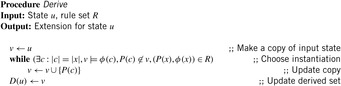
The semantics, roughly, are that an instance of a derived predicate is satisfied if and only if it can be derived using the available rules. More formally, let R be the set of rules for the derived predicates, where the elements of R have the form  – if ϕ(x) then
 . Then
  , for a set of basic facts u, is defined as follows:
 This definition uses the standard notations of the modeling relation
  between states (represented as sets of facts in our case) and formulas, and of the substitution ϕ(c) of the free variables in formula ϕ(x) with a constant vector c. In words, D(u) is the intersection of all supersets of u that are closed under application of the rules R. D(u) can be computed by the simple process shown in Algorithm 15.5. Hence, derivation rules can be included in a forward chaining heuristic search planner by inferring the truth of the derived rule for each step.
Suppose that we have grounded all derived predicates to the rules  . In ϕ there can be further derived predicates, which by the acyclic definition of derived predicates cannot be directly or indirectly dependent from p. For the rule
  the values p and ϕ are equivalent. This implies that p is nothing more than a macro for the expression ϕ. All derived predicates can be eliminated from the planning instance by the substitution with more complex descriptions. The advantage with regard to alternative methods for handling derived predicates is that the state vector does not have to be extended.
15.2.5. Timed Initial Literals
Timed initial literals are an extension for temporal planning. Syntactically they are a very simple way of expressing a certain restricted form of exogenous events: facts that will become true or false at time points that are known to the planner in advance, independent of the actions that the planner chooses to execute. Timed initial literals are thus deterministic unconditional exogenous events.
An illustrative example considers a planning task for shopping. There is a single action that achieves the goal, which requires a shop to be open as its precondition. The shop opens at time step 9 relative to the initial state, and closes at time step 20. We can express the shop opening times by two timed initial literals:
(:init (at 9 (shop-open)) (at 20 (not (shop-open)))).
Timed initial literals can be inserted into a heuristic search planner as follows. We associate with each (grounded) action so-called action execution time windows that specify the interval of a save execution. This is done by eliminating the preconditions that are related to the time initial literal. For ordinary literals and Strips actions, the conjunction of precondition leads to the intersection of action execution time windows. For repeated literals or disjunctive precondition lists, time windows have to be kept, while simple execution time windows can be integrated into the PERT scheduling process.
15.2.6. State Trajectory Constraints
State trajectory or plan constraints provide an important step of PDDL toward temporal control knowledge and temporally extended goals. They assert conditions that must be satisfied during the execution of a plan. Through the decomposition of temporal plans into plan happenings, state trajectory constraints feature all levels of the PDDL hierarchy. For example, the constraint a fragile block can never have something above it can be expressed as
(always (forall (?b - block) (implies (fragile ?b) (clear ?b)))).
As illustrated in Chapter 13 plan constraints can be compiled away. The approach translates the constraints in linear temporal logic and compiles them into finite-state automata. The automata are simulated in parallel to the search. The initial state of the automaton is added to the initial state of the problem and the automation transitions are compiled to actions. A synchronization mechanism controls that the original actions and the automata actions alternate. Planning goals are extended with the accepting states of the automata.
15.2.7. Preference Constraints
Annotating individual goal conditions or state trajectory constraints with preferences model soft constraints and allow the degree of satisfaction to be scaled with respect to hard constraints that have to be fulfilled in a valid plan. The plan objective function includes special variables referring to the violation of the preference constraints and allows planners to optimize plans.
Quantified preference rules like
(forall (?b - block) (preference p (clear ?b)))
are grounded (one for each block), while the inverse expression
(preference p (forall (?b - block) (clear ?b)))
leads to only one constraint.
Preferences can be treated as variables using conditional effects, so that the heuristics derived earlier remain appropriate for effective plan-finding.
15.3. Bibliographic Notes
Drew McDermott and a committee have created the specification language (PDDL) in 1998 in the form of a Lisp-like input language description format that includes planning formalisms like Strips by Fikes and Nilsson (1971). Later, ADL as proposed by Pednault (1991) was used. Planning in temporal and metric domains started in 2002. For this purpose, Fox and Long (2003) developed the PDDL hierarchy, of which the first three levels were shown in the text. This hierarchy was attached later. Domain axioms in the form of derived predicates introduce inference rules, and timed initial facts allow deadlines to be specified (Hoffmann and Edelkamp, 2005). Newer developments of PDDL focus on temporal and preference constraints (Gerevini and Long, 2005) and object fluents (Geffner, 2000). Complexity analyses for standard benchmarks have been provided by Helmert (2003) and Helmert (2006a). Approximation properties of such benchmarks have been studied by Helmert, Mattmüller, and Röger (2006). The complexity of planning with multivalued variables (SAS+ planning) has been analyzed by Bäckström and Nebel (1995).
Graphplan has been developed by Blum and Furst (1995) and Satplan is due to Kautz and Selman (1996). The set of admissible heuristics based on dynamic programming have been proposed by Haslum and Geffner (2000). Planning with pattern databases has been invented by Edelkamp (2001a) and the extension to symbolic pattern databases has been addressed by Edelkamp (2002). Various packing algorithms have been suggested by Haslum, Bonet, and Geffner (2005). Incremental hashing for planning pattern databases has been proposed by Mehler and Edelkamp (2005). The automated pattern selection for domain-independent explicit-state and symbolic heuristic search planning with genetic algorithms has been proposed by Edelkamp (2007). Zhou and Hansen (2006b) have used general abstractions for planning domains together with structured duplicate detection (see Ch. 8).
The relaxed planning heuristic as proposed by Hoffmann and Nebel (2001) has been analyzed by Hoffmann (2001), providing a heuristic search topology for its effectiveness in known benchmark domains. Bonet and Geffner (2008) have derived a functional representation of the relaxed planning heuristic in symbolic form as a DNNF. Alcázar, Borrajo, and Linares López (2010) have proposed using information extracted from the last actions in the relaxed plan to generate intermediate goals backward.
Hoffmann (2003) has shown how to extend the heuristic by omitting the delete list to numerical state variables. An extension of the approach to nonlinear tasks has been given by Edelkamp (2004). A unified heuristic for deterministic planning has been investigated by Rintanen (2006). Coles, Fox, Long, and Smith (2008) have refined the heuristic by solving linear programs to improve the relaxation. Fuentetaja, Borrajo, and Linares López (2008) have introduced an approach for dealing with cost-based planning that involves the use of look-ahead states to boost the search, based on a relaxed plan graph heuristic. How to add search diversity to the planning process has been studied by Linares López and Borrajo (2010).
Borowsky and Edelkamp (2008) have proposed an optimal approach to metric planning. State sets and actions are encoded as Presburger formulas and represented using minimized finite-state machines. The exploration that contributes to the planning via a model checking paradigm applies symbolic images to compute the finite-state machine for the sets of successors.
The causal graph heuristic has been discussed extensively by Helmert (2006b) and been implemented in the Fast-Downward planner. Helmert and Geffner (2008) have shown that the causal graph heuristic can be viewed as a variant of the max-atom heuristic with additional context. They have provided a recursive functional description of the causal graph heuristic that, without restriction to the dependency graph structure, extends the existing one.
Automated planning pattern database design has been studied by Haslum, Botea, Helmert, Bonet, and Koenig (2007). A more flexible design that goes back to work by Dräger, Finkbeiner, and Podelski (2009) has been pursued by Helmert, Haslum, and Hoffmann (2007) and pattern database heuristics for nondeterministic planning have been studied by Mattmüller, Ortlieb, Helmert, and Bercher (2010). In Katz and Domshlak (2009) structural pattern database heuristics have been proposed that lead to polynomial-time calculations based on substructures of the causal graph. Moreover, a general method for combining different heuristics has been given. Good heuristics have also been established by the extraction of landmarks in Richter, Helmert, and Westphal (2008), a work that refers to Hoffmann, Porteous, and Sebastia (2004). A theoretical analysis of the advances in the design of heuristics has lead to the heuristic LM-cut with very good results (Helmert and Domshlak, 2009). Bonet and Helmert (2010) have improved this heuristic by computing hitting sets.
Alternative characterizations that have been derived of hm have been given by Haslum (2009). Limits of heuristic search in planning domains have been documented by Helmert and Röger (2008).
Pruning techniques for the use of actions have been studied by Wehrle, Kupferschmid, and Podelski (2008). A reduced set of actions has been looked at in Haslum and Jonsson (2000). It is known that achieving approximate solutions in Blocksworld is easy (Slaney and Thiébaux, 2001) and that domain-dependent cuts drastically reduce the search space. For compiling temporal logic control into PDDL, Rintanen (2000) has compared formula progression as in TLPlan by Bacchus and Kabanza (2000) with a direct translation into planning actions.
For efficient optimization in complex domains, planner LPG by Gerevini, Saetti, and Serina (2006) and SGPlan by Chen and Wah (2004) apply Lagrangian optimization techniques to gradually improve a (probably invalid) first plan. Both planners extend the relaxed planning heuristics; the first one optimizes an action graph data structure, and the latter applies constraint partitioning (into less restricted subproblems). As shown in Gerevini, Saetti, and Serina (2006), the planner LPG-TD can efficiently deal with multiple action time windows. The outstanding performance of constraint partitioning, however, is likely due to manual help.
Further planers like Crikey by Coles, Fox, Halsey, Long, and Smith (2009) link planning and scheduling algorithms into a planner that is capable of solving many problems with required concurrency, as defined by Cushing, Kambhampati, Mausam, and Weld (2007). Alternatively, we can build domain-independent (heuristic) forward chaining planners that can handle durative actions and numeric variables. Planners like Sapa by Do and Kambhampati (2003) follow this approach. Sapa utilizes a temporal version of planning graphs first introduced in TGP by Smith and Weld (1999) to compute heuristic values of time-stamped states. A more recent approach has been contributed by Eyerich, Mattmüller, and Röger (2009).
..................Content has been hidden....................
You can't read the all page of ebook, please click here login for view all page.