Search in book...
Toggle Font Controls
Create new playlist

Name your new playlist

Playlist description (optional)
Sign In

Email address

Password

Forgot Password?

or

Continue with Facebook

Continue with Google
Sign Up

Full Name

Email address

Confirm Email Address

Password

or

Continue with Facebook

Continue with Google

Chapter 4. Automatically Created Heuristics

This chapter studies the limits and possibilities of problem abstractions and their relation to heuristic search. As the most important representative of abstraction data structures, it considers pattern databases in a great level of detail.

Keywords: abstraction, Voltorta's theorem, hierarchical A*, pattern database, multiple pattern database, disjoint pattern database, additive pattern database, symmetry pattern database, dual pattern database, bounded pattern database, on-demand pattern database, compressed pattern database, compact pattern database.

Where do heuristics come from? A common view is that heuristics are relaxations of constraints of the problem that solve a relaxed problem exactly. A prominent example for this is the straight-line distance estimate for routing problems. It can be interpreted as adding straight routes to the map. The notion of an abstraction transformation formalizes this concept, and makes it accessible to an automated generation of heuristics, as opposed to hand-crafted, domain-dependent solutions using human intuition. However, a negative result shows that such transformations cannot lead to a speed-up on their own; on the contrary, the power of abstractions lies in the reduction of multiple concrete states to a single abstract state.

Although earlier versions of heuristic search via abstraction generated heuristic estimates on-the-fly, pattern databases precompute and store the goal distances for the entire abstract search space in a lookup table. Successful approaches additionally combine the heuristics of multiple smaller pattern databases, either by maximizing or by cumulating the values, which is admissible under certain disjointness conditions. To save space, the computation of the database can be restricted using an upper bound on the length of an optimal solution path and by exploiting specialized data compression schemes.

Therefore, abstraction is the key to the automated design of heuristic estimates. Applying abstractions simplifies the problem, and the exact distances in the simplified version serve as heuristic estimates in the concrete state space. The combination of heuristics based on different abstractions often leads to better estimates. In some cases an abstraction hierarchy can be established. The selection of abstraction functions is usually supervised by the user, but first, progress in computing abstractions automatically are shown.

Abstraction is a method to reduce the exploration efforts for large and infinite state spaces. The abstract space is often smaller than the concrete one. If the abstract system has no solution, neither has the concrete one. However, abstractions may introduce so-called spurious solution paths, the inverse of which is not present in the concrete system. One option to deal with the problem of spurious solution paths is the design of an abstract-and-refine loop, in which the coarse abstraction is refined for one that is consistent with the solution path established, so that the search process can start again. In contrast, we exploit the duality of abstraction and heuristic search. Abstract state spaces are explored to create a database that stores the exact distances from abstract states to the set of abstract goal states. Instead of checking whether or not the abstract path is present in the concrete system, efficient heuristic state space search algorithms exploit the database as a guidance. Many abstractions remove state variables, others are based on data abstraction. They assume a state vector with state components of finite domain and map these domains to abstract variables with smaller domain.

4.1. Abstraction Transformations

In AI search, researchers have investigated abstraction transformations as a way to create admissible heuristics automatically.

Definition 4.1

(Abstraction Transformation) An abstraction transformation

maps states u in the concrete problem space to abstract states

and concrete actions a to abstract actions

If the distance between all states

in the concrete space is greater than or equal to the distance between

and

, the distance in the abstract space can be used as an admissible heuristic for the concrete search space. It is possible to either compute the heuristic values on demand, as in hierarchical A* (see Sec. 4.3), or to precompute and store the goal distance for all abstract states when searching with pattern databases (see Sec. 4.4).

Intuitively, this agrees with a common explanation of the origin of heuristics, which views them as the cost of exact solutions to a relaxed problem. A relaxed problem is one where we drop constraints (e.g., on move execution). This can lead to inserting additional edges in the problem graph, or to a merging of nodes, or both.

For example, the Manhattan distance for sliding-tile puzzles can be regarded as acting in an abstract problem space that allows multiple tiles to occupy the same square. At first glance, by this relaxation there could be more states than in the original, but fortunately the problem can be decomposed into smaller problems.

Two frequently studied types of abstraction transformations are embeddings and homomorphisms.

Definition 4.2

(Embedding and Homomorphism) An abstraction transformation ϕ is an embedding transformation if it adds edges to S such that the concrete and abstract state sets are the same; that is,

for all

. Homomorphism requires that for all edges

in S, there must also be an edge

in S′.

By definition, embeddings are special cases of homomorphisms, since existing edges remain valid in the abstract state space. Homomorphisms group together concrete states to create a single abstract state. The definition is visualized in Figure 4.1.

Some rare abstractions are solution preserving, meaning a solution path in the abstract problem also introduces a solution path in the concrete problem. In this case, the abstraction does not introduce spurious paths. As a simple example for introducing a spurious path consider edges

and

in the concrete space. Then there is no path from x to y in the concrete space, but there is one after merging u and v.

For an example of a solution-preserving abstraction, we assume that v is the only successor of u and that the abstraction would merge them. The concrete edge from u to v is converted to a self-loop and thus introduces infinite paths in the abstract space. However, a solution path exists in the abstract problem if and only if a solution path exists in the concrete problem.

Some solution-preserving reductions are not homomorphic. For example, consider that two paths

and

in the concrete state space are reduced to

and

in the abstract state spaces. In other words, diamond subgraphs are broken according to move transpositions.

Another issue is whether the costs of abstract paths are lower or equal. In our case, we generally assume that the cost of the actions in abstract space are the same as in concrete space. In most cases, we refer to unit cost problem graphs. The usefulness of heuristics derived from abstraction transformations is due to the following result.

B9780123725127000043/f04-01-9780123725127.jpg is missing

Figure 4.1

Concrete states and connecting edge mapped to abstract states and connecting edge via a state space homomorphism. Note that the concrete state space can be much larger than the abstraction, inducing a potentially large group of states mapped to the identical abstract state.

Theorem 4.1

(Admissibility and Consistency of Abstraction Heuristics) Let S be a state space and

be any homomorphic abstraction transformation of S. Let heuristic function

for state u and goal t be defined as the length of the shortest path from

in S′. Then

is an admissible, consistent heuristic function.

Proof

is a shortest solution in S,

is a solution S′, which obviously cannot be shorter than the optimal solution in S′.

Now recall that a heuristic h is consistent, if for all u and u′ in S,

. Because

is the length of the shortest path between

and

, we have

for all u and u′. Substituting

results in

for all u and u′. Because ϕ is an abstraction,

and, therefore,

for all u and u′.

The type of abstraction usually depends on the state representation. For example, in logical formalisms, such as Strips, techniques that omit a predicate from a state space description induce homomorphisms. These predicates are removed from the initial state and goal and from the precondition (and effect) lists of the actions.

The Star abstraction is another general method of grouping states together by neighborhood. Starting with a state u with the maximum number of neighbors, an abstract state is constructed of which the range consists of all the states reachable from u within a fixed number of edges.

Another kind of abstraction transformations are domain abstractions, which are applicable to state spaces described in PSVN notation, which was introduced in Section 1.8.2. A domain abstraction is a mapping of labels

. It induces a state space abstraction by relabeling all constants in both concrete states and actions; the abstract space consists of all states reachable from

by applying sequences of abstract actions. It can be easily shown that a domain abstraction induces a state space homomorphism.

For instance (see Fig. 4.2), consider the Eight-Puzzle with vector representation, where tiles 1, 2, and 7 are replaced by the don't care symbol x. We have

with

, and

, otherwise. In addition to mapping tiles 1, 2, and 7 to x, in another domain abstraction ϕ₂ we might additionally map tiles 3 and 4 to y, and tiles 6 and 8 to z. The generalization allows refinements to the granularity of the relaxation, defined as a vector indicating how many constants in the concrete domain are mapped to each constant in the abstract domain. In the example, the granularity of ϕ₂ is

because three constants are mapped to x, two are mapped to each of y and z, and constants 5 and 0 (the blank) remain unique.

B9780123725127000043/f04-02-9780123725127.jpg is missing

Figure 4.2

Two abstractions of the Eight-Puzzle; top abstraction maps all involved tiles to one don't care symbol x; in the bottom abstraction, two tile labels x and y have been introduced.

In the sliding-tile puzzles, a granularity

implies that the size of the abstract state space is

, with the choice of

depending on whether or not half of all states are reachable due to parity (see Sec. 1.7). In general, however, we cannot directly derive the size from the granularity of the abstraction: ϕ might not be surjective; for some abstract states u′ there might not exist a concrete state u such that

. In this case, the abstract space can even comprise more states than the original one, thereby rendering the method counterproductive. In general, unfortunately, it is not efficiently decidable if an abstract space is surjective.

4.2. Valtorta's Theorem

Without a heuristic, we can only search blindly in the original space; the use of a heuristic focuses this search, and saves us some computational effort. However, this is only beneficial if the cost of the auxiliary search required to compute h doesn't exceed these savings. Valtorta found an important theoretical limit of usefulness.

Theorem 4.2.

(Valtorta's Theorem) Let u be any state necessarily expanded, when the problem

is solved in S with BFS;

be any abstraction mapping; and the heuristic estimate

be computed by blindly searching from

. If the problem is solved by the A* algorithm using h, then either u itself will be expanded, or

will be expanded.

Proof

When A* terminates, u will either be closed, open, or unvisited.

• If u is closed, it has already been expanded.

• If u is open, then

must have been computed during search.

is computed by searching in S′ starting at

; if

, the first step in this auxiliary search is to expand

; otherwise, if

then

, and u itself is necessarily expanded.

• If u is unvisited, on every path from s to u there must be a state that was added to Open during search but never expanded.

Let v be any such state on the shortest path from s to u. Because v was opened,

must have been computed. We will now show that in computing

is necessarily expanded.

From the fact that u is necessarily expanded by blind search, we have

. Because v is on the shortest path, we have

. From the fact that v was never expanded by A*, we have

. Combining the two inequalities, we get

. Since ϕ is an abstraction mapping, we have

, which gives

. Therefore,

is necessarily expanded.

As a side remark note that Valtorta's theorem is sensitive to whether the goal counts as expanded or not. Many textbooks including this one assume that A* stops immediately before expanding the goal.

Since

in an embedding, we immediately obtain the following consequence of Valtorta's theorem.

Corollary 4.1

For an embedding ϕ, A*—using h computed by blind search in the abstract problem space—necessarily expands every state that is expanded by blind search in the original space.

Of course, this assumes that the heuristic is computed once for a single problem instance; if it were stored and reused over multiple instances, its calculation could be amortized.

Contrary to the case of embeddings, this negative result of Valtorta's theorem does not apply in this way to abstractions based on homomorphisms; they can reduce the search effort, since the abstract space is often smaller than the original one.

As an example, consider the problem of finding a path between the corners

and

on a regular N × N Gridworld, with the abstraction transformation ignoring the second coordinate (see Fig. 4.3 for N = 10; the reader may point out the expanded nodes explicitly and compare with nodes expanded by informed search). Uninformed search will expand

nodes. On the other hand, an online heuristic requires

steps. If A* applies this heuristic to the original space, and resolves ties between nodes with equal f-value by preferring the one with a larger g-value, then the problem demands

expansions.

B9780123725127000043/f04-03-9780123725127.jpg is missing

Figure 4.3

Two-dimensional Gridworld problem with initial state (1, 1) and goal state (10, 1) illustrating the validity of Valtorta's theorem; the abstraction projects a state to its x-axis, such that the h-value is the size of the line from the projected point to the goal.

4.3. Hierarchical A

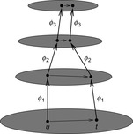
Hierarchical A* makes use of an arbitrary number of abstraction transformation layers

. Whenever a heuristic value for a node u in the base level problem is requested, the abstract problem to find a shortest path between

and

is solved on demand, before returning to the original problem. In turn, the search at level 2 utilizes a heuristic computed on a third level as the shortest path between

and

, and so on (see Fig. 4.4).

This naive scheme would repeatedly solve the same instances at the higher levels requested by different states at the base level. An immediate remedy for this futile overhead is to cache the heuristic values of all the nodes in a shortest path computed at an abstract level.

B9780123725127000043/f04-04-9780123725127.jpg is missing

Figure 4.4

Layered abstraction in hierarchical A* with regard to the current state u and goal state t (in the original state space) according to three abstractions.

The resulting heuristic will no longer be monotone: Nodes that lay on the solution path of a previous search can have high h-values, whereas their neighbors off this path still have their original heuristic value. Generally, a nonmonotone heuristic leads to the need for reopening nodes; they can be closed even if the shortest path to them has not yet been found. However, this is not a concern in this case: A node u can only be prematurely closed if every shortest path passes through some node v for which the shortest path is known. If no such v is part of a shortest path from s to t, neither is u, and the premature closing is irrelevant. On the other hand, all nodes on the shortest path from v to t have already cached the exact estimate, and hence will only be expanded once.

An optimization technique, known as optimal path caching, records not only the value of

, but also the exact solution path found. Then, whenever a state u with known value

is encountered during the search, we can directly insert a goal into the Open list, instead of explicitly expanding u.

In controlling the granularity of abstractions, there is a trade-off to be made. A coarse abstraction leads to a smaller problem space that can be searched more efficiently; however, since a larger number of concrete states are assigned the same estimate, the heuristic becomes less discriminating and hence less informative.

4.4. Pattern Databases

In the previous setting, heuristic values are computed on demand. With caching, a growing number of them will be stored over time. An alternative approach is to completely evaluate the abstract search space prior to the base level search. For a fixed goal state t and any abstraction space

, a pattern database is a lookup table indexed by

containing the shortest path length from u′ to

in S′ for

. The size of a pattern database is the number of states in S′.

It is easy to create a pattern database by conducting a breadth-first search in a backward direction, starting at

. This assumes that for each action a we can devise an inverse action a⁻¹ such that

iff

. If the set of backward actions

is equal to A, the problem is reversible (leading to an undirected problem graph). For backward pattern database construction, the uniqueness of the actions’ inverse is sufficient. The set of all states generated by applying inverse actions to a state u is denoted as

. It is generated by the inverse successor generating function

. Pattern databases can cope with weighted state spaces. Moreover, by additionally associating the shortest path predecessor with each state it is possible to maintain the shortest abstract path that leads to the abstract goal. To construct a pattern database for weighted graphs, the shortest path exploration in abstract space uses inverse actions and Dijkstra's algorithm.

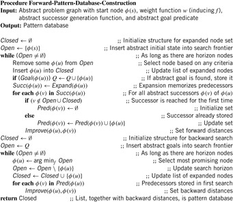
Algorithm 4.1 shows a possible implementation for pattern database construction. It is not difficult to see that the construction is in fact a variant of Dijktra's algorithm (as introduced in Ch. 2) executed backward in abstract space (with successor set generation

instead of

for abstract states

instead of u). Even though in many cases pattern databases are constructed for a single goal state t it extends nicely the search for multiple goal states T. Therefore, in Algorithm 4.1Open is initialized with T.

For the sake of readability in the pseudo codes we often use the set notation for the accesses to the Open and Closed lists. In an actual implementation, the data structures of Chapter 3 have to be used. This pattern database construction procedure is sometimes termed retrograde analysis.

B9780123725127000043/u04-01-9780123725127.jpg is missing

Algorithm 4.1.

Construction of pattern database using a backward search.

Since pattern databases represent the set Closed of expanded nodes in abstract space, a straightforward implementation for storing and retrieving the computed distance information are hash tables. As introduced in Chapter 3, many different options are available such as hash tables with chaining, open addressing, suffix lists, and others. For search domains with a regular structure (like the (n²−1)-Puzzle), the database can be time- and space-efficiently implemented as a perfect hash table. In this case the hash address uniquely identifies the state that is searched, and the hash entries themselves consist of the shortest path distance value only. The state itself has not been stored. A simple and fast (though not memory-efficient) implementation of such a perfect hash table is a multidimensional array that is addressed by the state components. More space-efficient indexes for permutation games have been introduced in Chapter 3. They can be adapted to partial state/pattern addresses.

The pattern database technique was first applied to define heuristics for sliding-tile puzzles. The space required for pattern database construction can be bounded by the length of the abstract goal distance encoding times the size of the perfect hash table.

4.4.1. Fifteen-Puzzle

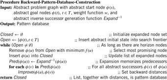
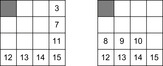
For this case, problem abstraction consists of ignoring a selected subset of tiles on the board. Their labels are replaced by a special “don't care” symbol; the remaining set of tiles is referred to as the pattern. Sample fringe and corner patterns are illustrated in Figure 4.5.

B9780123725127000043/f04-05-9780123725127.jpg is missing

Figure 4.5

Fringe and corner target pattern for the Fifteen-Puzzle.

In experiments it has been shown that taking the maximum of the Manhattan distance and the fringe (corner) pattern database reduces the number of expanded nodes by two orders of magnitude of the algorithm using only the Manhattan distance. Using both databases together even leads to an improvement according to three orders of magnitude. Table 4.1 shows further exploration results for the Fifteen-Puzzle in reducing the number of search nodes and increasing mean heuristic value.

**Table 4.1** Effect of pattern databases in the Fifteen-Puzzle.
Heuristic	Nodes	Mean Heuristic Value
Manhattan Distance	401,189,630	36.942
Linear Conflict Heuristic	40,224,625	38.788
5-Tile Pattern Database	5,722,922	41.562
6-Tile Pattern Database	3,788,680	42.924

4.4.2. Rubik's Cube

A state in Rubik's Cube (see Sec. 1.7.2) is uniquely specified by the position and orientation of the 8 edge cubies and the 12 corner cubies. For the implementation, this can be represented as an array of 20 elements, one for each cubie. The values encode the position and orientation as one of 24 different values—8.3 for the corners and 2·12 for the edges.

Uninformed search is impractical on large Rubik's Cube problems, since the number of generated nodes grows rapidly. In Depth 10 we expect 244,686,773,808 nodes, and in Depth 18 we have more than 2.46·10²⁰ nodes.

If we consider the eight corner cubies as a pattern, the position and orientation of the last cubie is determined by the remaining seven, so there are exactly

possible combinations. Using backward breadth-first search starting from the goal state, we can enumerate these states and build a pattern database. Perfect hashing can be used, allocating four bits to encode the heuristic value for each abstract state. The mean heuristic value is about 8.764. In addition, we may consider the edge cubies separately. Since taking all edge cubies into consideration would lead to a memory-exceeding pattern database, the set of edge cubies is divided, leading to two pattern databases of size

. The mean heuristic value for the maximum of all three pattern database heuristics is about 8.878.

Using the previous databases, Korf solved 10 random instances to the Rubik's Cube move optimally. The solvable instances were generated by making 100 random moves each starting from the goal state. His results are shown in Table 4.2. The optimal solution for the hardest possible instance has 20 moves (see Ch. 1).

**Table 4.2** Solutions to 10 random Rubik's Cube instances.
Problem	Depth	Nodes Generated
1	16	3,720,885,493
2	17	11,485,155,726
3	17	64,937,508,623
4	18	126,005,368,381
5	18	262,228,269,081
6	18	344,770,394,346
7	18	502,417,601,953
8	18	562,494,969,937
9	18	626,785,460,346
10	18	1,021,814,815,051

4.4.3. Directed Search Graphs

A precondition for the above construction is that actions are inversible; that is, the set of legal reachable states that can be transformed into a target state must be efficiently computable. This is true for regular problems like the (n²−1)-Puzzle and Rubik's Cube. However, applying inversible actions is not always possible. For example, in PSVN the action

is not inversible, since in a backward direction, it is not clear which label to set at the first and second position (although we know it must be the same one). In other words, we no longer have an inverse abstract successor generation function to construct set Pred.

Fortunately, there is some hope. If inverse actions are not available, we can reverse the state space graph generated in a forward chaining search. With each node v we attach the list of all predecessor nodes u (assuming

) from which v is generated. In case a goal is encountered, the traversal is not terminated, but the abstract goal states are collected in a (priority) queue. Next, backward traversal is invoked on the inverse of the (possibly weighted) state space graph, starting with the queued set of abstract goal states. The established shortest path distances to the abstract goal state are associated with each state in the hash table. Algorithm 4.2 shows a possible implementation. Essentially, a forward search to explore the whole state space is executed, memorizing the successors of all states, so that we can then construct their predecessors. Then we perform Backward-Pattern-Database-Construction without the need to apply inverse node expansion.

4.4.4. Korf's Conjecture

In the following we are interested in the performance of pattern databases. We will argue that for the effectiveness of an (admissible) heuristic function, the expected value is a very good predictor. This average can be approximated by random sampling, or for pattern databases determined as the average of the database values. This value is exact for the distribution of heuristic values in the abstract state space but, as abstractions are nonuniform in general, only approximate for the concrete state space.

B9780123725127000043/u04-02-9780123725127.jpg is missing

Algorithm 4.2.

Pattern database construction in directed and weighted problem graphs.

In general, the larger the values of an admissible heuristic, the better the corresponding database should be judged. This is due to the fact that the heuristic values directly influence the search efficiency in the original search space. As a consequence, we compute the mean heuristic value for each database. More formally, the average estimate of a pattern database PDB with entries in the range

A fundamental question about memory-based heuristics concerns the relationship between the size of the pattern database and the number of nodes expanded when the heuristic is used to guide the search. One problem of relating the performance of a search algorithm to the accuracy of the heuristic is it is hard to measure. Determining the exact distance to the goal is computationally infeasible for large problems.

If the heuristic value of every state is equal to its expected value

, then a search to depth d is equivalent to searching to depth

without a heuristic, since the f-value for every state would be its depth plus

. However, this estimate turns out to be much too low in practice. The reason for the discrepancy is that the states encountered are not random samples. States with large heuristic values are pruned and states with small heuristic values spawn more children.

On the other hand, we can predict the expected value of a pattern database heuristic during the search. The minimal depth of a search tree covering a search space of n nodes with constant branching factor of b will be around

. This is because with d moves, we can generate about

nodes. Since we are ignoring possible duplicates, this estimate is generally too low.

We assume d to be the average optimal solution length for a random instance and that our pattern database is generated by caching heuristic values for all states up to distance d from the goal. If the abstract search tree is also branching with factor b, a lower bound on the expected value of a pattern database heuristic is

, where m is the number of stored states in the database (being equal to the size of the abstract state space). The derivation of

is similar to the one of

for the concrete state space.

The hope is that the combination of an overly optimistic estimate with a too-pessimistic estimate results in a more realistic measure. Let t be the number of nodes generated in an A* search (without duplicate detection). Since d is the depth to which A* must search, we can estimate

. Moreover, as argued earlier, we have

and

. Substituting the values for d and

yields

Since the treatment is insightful but informal, this estimate has been denoted as Korf's conjecture; it states that the number of generated nodes in an A* search without duplicate detection using a pattern database may be approximated by

, the size of the problem space divided by the available memory. Using experimental data from the Rubik's Cube problem shows that the prediction is very good. We have

, and

, which is off only by a factor of 1.4.

4.4.5. Multiple Pattern Databases

The most successful applications of pattern databases all use multiple ones.

This raises the question on improved main memory consumption: Is it best to use one large database, or rather split the available space up into several smaller ones? Let m be the number of patterns that we can store in the available memory, and p be the number of pattern databases. In many experiments on the performance of p pattern databases of size

(e.g., in the domain of the sliding-tile puzzle and in Rubik's Cube) it has been observed that small values of p are suboptimal. The general observation is that the use of maximized smaller pattern databases reduces the number of nodes. For example, heuristic search in the Eight-Puzzle with 20 pattern databases of size 252 performs less state expansions (318) than 1 pattern database of size 5,040 (yielding 2,160 state expansions).

The observation remains true if maximization is performed on a series of different partitions into databases. The first heuristic of the Twenty-Four-Puzzle partitions the tiles into four groups of 6 tiles each. When partitioning the 24 tiles into eight different pattern databases with four groups of 5 tiles and one group of 4 tiles this results

patterns. Compared to the first heuristic that generates

patterns, this is roughly one-third. However, the second heuristic performs better, with a ratio of nodes generated in between 1.62 to 2.53.

Of course, the number of pattern databases cannot be scaled to an arbitrary amount. With very few states the distances in abstract state space are very imprecise. Moreover, since node generation in sliding-tile puzzles is very fast, the gains of a smaller node count are counterbalanced by the larger efforts in addressing the multiple databases and computing the maximum.

The explanation of this phenomenon, that many smaller pattern databases may perform better than one larger one, is based on two observations:

• The use of smaller pattern databases instead of one large pattern database usually reduces the number of patterns with high h-value; maximizing the values of the smaller pattern databases can make the number of patterns with low h-values significantly smaller than the number of low-valued patterns in the larger pattern database.

• Eliminating low h-values is more important for improving search performance than for retaining large h-values.

The first assertion is intuitively clear. A smaller pattern database means a smaller pattern space with fewer patterns with high h-values. Maximization of the smaller pattern databases reduces the number of patterns with very small h-values.

The second assertion refers to the number of nodes expanded. If pattern databases differ only in their maximum value, this only affects the nodes with a large h-value, corresponding to a number of nodes that is typically small. If the two pattern databases, on the contrary, differ in the fraction of nodes with a small h-value, this has a large effect on the number of nodes expanded, since the number of nodes that participate in those values is typically large.

As multiple pattern database lookups can be time consuming, we gain efficiency by computing bounds on the heuristic estimate prior to the search, and avoiding database lookups if the bounds are exceeded.

4.4.6. Disjoint Pattern Databases

Disjoint pattern databases are important to derive admissible estimates. It is immediate that the maximum of two heuristics is admissible. On the other hand, we would like to add the heuristic estimates of two pattern databases to arrive at an even better estimate. Unfortunately, adding heuristics does not necessarily preserves admissibility. Additivity can be applied if the cost of a subproblem is composed from costs of objects from a corresponding pattern only. For the (n² − 1)-Puzzle, every operator moves only one tile, but Rubik's Cube is a counterexample.

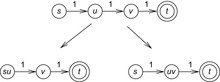
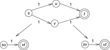
Consider the example of a small graph with four nodes s, u, v, and t arranged along one path (see Fig. 4.6), where s is the start and t is the goal node. The first abstraction merges nodes s and u, and the second abstraction merges u with v. Because self-loops do not contribute to optimal solutions they have been omitted from the abstract graph. As the incoming edge to t remains in both abstractions, being in state v gives the cumulated abstract distance value 2, which is larger than the concrete distance 1.

B9780123725127000043/f04-06-9780123725127.jpg is missing

Figure 4.6

Two nonadditive abstractions of a graph (top) obtained by merging nodes s with u (left) and u with v (right).

The reason why we could only take the maximum of the fringe and corner heuristics for the Eight-Puzzle is that we want to avoid counting some action twice. The minimum number of moves stored in the database does not involve only the tiles' movements that are part of the actual pattern. Since the nonpattern moves can be part of the abstract solution path for the other pattern, adding the two values might result in a nonadmissible heuristic.

A solution for the problem is not to record the total solution path length, but to count moves of the tiles in the pattern for computing the heuristic estimate only. Since at each point in time only one tile is moved, this makes it possible to add the heuristic values rather than maximizing them. As an extreme case, we can think of the Manhattan distance as the sum of n² − 1 patterns consisting of one tile each. Since each move changes only the shifted tile, addition is admissible. Generally, we can resort to this partitioning technique if we make sure that the subgoal solutions are independent.

Different disjoint pattern databases' heuristics can additionally be combined using the maximization of their outcome. For example, when solving random instances of the Twenty-Four-Puzzle, we might compute the maximum of two additive groups of four disjoint pattern databases each. As shown in Figure 4.7 each tile group (indicated by the enclosed areas) consists of six tiles for generating databases with

patterns (the location of the blank is indicated using a black square).

Figure 4.7

Disjoint pattern databases for a 24-Puzzle; tiles (in the goal) selected for the pattern are shown together.

If, for all states, the same partitioning is applied, we speak of statically partitioned disjoint pattern databases. There is an alternative way of dynamically choosing among several possible partitions the one with the maximum heuristic value. For example, a straightforward generalization of the Manhattan distance for sliding-tile puzzles is to precompute the shortest solution for every pair of tiles, rather than considering each tile individually. Then, we can construct an admissible heuristic by choosing half of these pairs such that each tile is covered exactly once. With an odd number of tiles, one of them will be left out, and simply contributes with its Manhattan distance.

To compute the most accurate heuristic for a given state, we have to solve a maximum weighted bipartite matching problem in a graph where each vertex in both sets corresponds to a tile, and each edge between the two sets is labeled with the pairwise solution cost of the corresponding pair of tiles. An algorithm is known that accomplishes this task in

time, where k is the number of tiles. However, it has also been shown that the corresponding matching problem for triples of tiles is NP-complete. Thus, in general, dynamic partitioning might not be efficiently computable, and we would have to resort to approximate the largest heuristic value.

If we partition the state variables into disjoint subsets (patterns), such that no action affects variables in more than one subset, then a lower bound for the optimal solution of an instance is the sum of the optimal costs of solving optimally each pattern corresponding to the variable values of the instance.

Definition 4.3

(Disjoint State Space Abstractions) Let actions be trivial (a no-op) if they induce a self-cycle in the abstract state space graph. Two state space abstractions ϕ₁ and ϕ₂ are disjoint, if for all nontrivial actions a′ in the abstraction generated by ϕ₁ and for all nontrivial actions

in the abstraction generated by ϕ₂, we have

, where

. Trivial actions correspond to self-loops in the problem graph.

If we have more than one pattern database, then for each state u in the concrete space and each abstraction

we compute the values

. The heuristic estimate

is the accumulated cost of the costs in the different abstractions; that is,

. To preserve admissibility, we require disjointness, where two pattern databases with regard to the abstractions

and

are disjoint, if or all

we have

Theorem 4.3

(Additivity of Disjoint Pattern Databases) Two disjoint pattern databases are additive, by means that their distance estimates can be added while still providing a lower bound for the optimal solution path length.

Proof

Let P₁ and P₂ be abstractions of

according to ϕ₁ and ϕ₂, respectively, and let

be an optimal sequential plan for P. Then, the abstracted plan

is a solution for the state space problem P₁, and

is a solution for the state space problem P₂. We assume that all void actions in

and

, if any, are removed. Let k₁ and k₂ be the resulting respective lengths of

and

. Since the pattern databases are disjoint, for all

and all

we have

. Therefore,

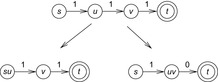
Consider a slight modification of the example graph with four nodes s, u, v, and t, now arranged as shown in Figure 4.8. The first abstraction merges nodes s with u and v with t and the second abstraction merges s with v and u with t. Now each edge remains valid in only one abstraction, so that being in state v gives the cumulated abstract distance value 1, which is equal to the concrete distance 1.

B9780123725127000043/f04-08-9780123725127.jpg is missing

Figure 4.8

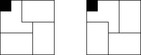
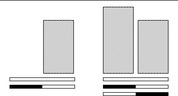
Disjoint abstractions of a small graph (top), obtained by merging nodes s with u and v with t (left) and s with v and u with t (right).

In Figure 4.10 a plain pattern database (left) and a pair of disjoint pattern databases (right) are shown. All pattern databases (gray bars) refer to underlying partial state vectors (represented as thin rectangles). The first rectangle in both cases represents the state vector in original space with all parts of it being relevant (no shading). The second (and third) rectangle additionally indicates the selected part of don't care variables in the state vector (shaded in black) for each abstraction. The heights of the pattern database bars that are erected on top of the state vector indicate the sizes of the pattern databases (number of states stored), and the widths of the pattern database rulers correlate with the selected parts of the state vector. The maximum size of a pattern database is determined by the amount of main memory available and is illustrated by a line above the databases.

B9780123725127000043/f04-09-9780123725127.jpg is missing

Figure 4.9

Admissible but nondisjoint abstraction of a small graph obtained by merging nodes s with u (left) and u with v (right), and adjusting the edge weights to avoid multiple-edge counting.

B9780123725127000043/f04-10-9780123725127.jpg is missing

Figure 4.10

Single (left) and two disjoint databases (right); height of bars denote size of the pattern database, horizontal line on top of the bars denote the limit of main memory, and the rulers below the bar denote selected pattern parts in a state vector (black stands for don't care variable, and white denotes a pattern variable).

Finding disjoint state space abstractions in general is difficult. Therefore, in pattern database practice, an alternative approach for enforcing disjointness is used: If an action has a nonempty intersection with one more than one chosen pattern, it is assigned to cost 0 in all but one database. Alternatively, we can assign 1 divided by the number of times the action is valid for an abstraction.

For the (n² − 1)-Puzzle at most one tile can move at a time. Hence, if we restrict the count to only pattern tile moves, we can add entries of pattern databases with a disjoint tile set. Table 4.3 shows the effect of disjoint pattern databases in reducing the number of search nodes and increasing the mean heuristic value.

**Table 4.3** Effect of disjoint pattern databases in the Fifteen-Puzzle.
Heuristic	Nodes	Mean Heuristic Value
Manhattan Distance	401,189,630	36.942
Disjoint 7- and 8-Tile Pattern Databases	576,575	45.632

Reconsider the example of the graph with four nodes s, u, v, and t arranged along a path with its two abstraction functions. The edge to t is assigned to cost 1 in the first abstraction and to cost 0 in the second abstraction such that, when being in state v, the cumulated abstract distance value is now 1, which is equal to the concrete distance 1. The resulting mapping is shown in Figure 4.9.

In general, we cannot expect that each action contributes costs to only one pattern database. For this case, concrete actions can be counted multiple times in different abstractions. This implies that the inferred heuristic is no longer admissible. To see this, suppose that this action immediately reaches the goal with cost 1. In contrast, the cumulated cost for being nonvoid in two abstractions is 2.

Another option is to count an action in only one abstraction. In a modified breadth-first pattern database construction algorithm this is achieved as follows. In each BFS level we compute the transitive hull of zero-cost actions: each zero-cost action is applied until no zero-cost action is applicable. In other words, the impact of an action is added to the overall cost, only if it does not appear for the construction of another pattern database.

A general theory of additive state space abstraction has been defined on top of a directed abstract graph by assigning two weights per edge, one for the primary cost

and residual cost

. Having two costs per abstract edge instead of just one is inspired by counting distinguished moves differently than don't care moves. In that example, our primary cost is the cost associated with the distinguished moves, and our residual cost is the cost associated with the don't care moves.

It is not difficult to see that if for all edges

and state space abstractions

in the original space the edge

is contained in the abstract space, and if for all paths

in the original space we have

, the resulting heuristic is consistent. Moreover, if for all paths

we have

, the resulting additive heuristic is also consistent.

4.5. * Customized Pattern Databases

So far we looked at manual selection of pattern variables. On the one hand, this implies that pattern-database design is not domain independent. On the other hand, finding good patterns for the design of one pattern database is involved, as there is an exponential number of possible choices. This problem of pattern selection becomes worse when general abstractions and multiple pattern databases are considered. Last, but not least, the quality of pattern databases is far from being obvious.

4.5.1. Pattern Selection

To automate the pattern selection process is a challenge. For domain-independent choices of the patterns, we have to control the size of the abstract state space that corresponds to this choice. State spaces for fixed-size state vectors can be interpreted as products of state space abstractions for individual state variables. An upper bound of the abstract state space is to multiply the preimages of the remaining variables.

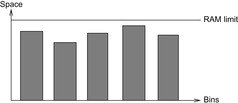
Upper bounds on the size of the abstract spaces can be used to distribute the pattern variables. Since the number of state variables can be considerably large, we simplify the problem of finding a suitable partition of the state vector into patterns to a form of Bin Packing. Consequently, the aim for automated pattern selection is to distribute the state variables to abstract state space bins in such a way that a minimal number of bins is used. A state variable is added to an already existing bin, until the (expected) abstract state space size exceeds main memory.

In constrast to ordinary Bin Packing that adds object sizes, the Pattern Packing variant is suited to automated pattern selection. For Pattern Packing the domain sizes to estimate the abstract state space growth multiply. More formally, adding a variable to a pattern corresponds to a multiplication of its domain size to the (already computed) abstract state size (unless it exceeds the RAM limit). As an example, the abstract state space for the variables v₁ and v₂ is bounded from above by

, where

denotes the set of possible assignments to

. Adding v₃ yields an upper bound for the abstract state space size of

Figure 4.11 illustrates an example, plotting the sizes of the pattern databases against the set of chosen abstractions. Bin Packing is NP-complete, but efficient approximations (like first- or best-fit strategies) have been used successfully in practice.

B9780123725127000043/f04-11-9780123725127.jpg is missing

Figure 4.11

Bin packing for automated pattern selection; bars illustrate the contents of each pattern of databases, and the horizontal line indicates the limit of main memory.

As argued earlier, a linear gain in the mean heuristic value

corresponds to an exponential gain in the search. For the pattern selection problem we conclude that the higher the average distance stored, the better the corresponding pattern database. For computing the strength of multiple pattern databases we compute the mean heuristic value for each of the databases individually and add (or maximize) the outcome.

In the following we show that there is a unique way of combining several pattern database heuristics into one.

Definition 4.4

(Canonical Pattern Database Heuristic) Let C be a collection of abstractions

and let X be a collection of all disjoint subsets Y of C maximal with respect to set inclusion. Let

be the pattern database for

. The canonical pattern database heuristic

is defined as

Theorem 4.4

(Consistency and Quality of Canonical Pattern Database Heuristic) The canonical pattern database heuristic is consistent and is larger than or equal to any admissible combination of maximums and sums.

Proof

Intuitively, the proof is based on the fact that for this case the maximum over all sums is equal to the sum over the maxima, such that no maximum remains nested inside. We illustrate this for two pattern databases. Suppose we are given four abstractions

with

and

being disjoint for

and

. Let

and

. We show

and

. Since for all u the value

is the maximum over all sums

and

, it cannot be less than the particular pair

that is selected in h′. Conversely, the maximum in

is attained by

for some

and

. As the pattern database heuristics are derived from different terms, this implies that

and

A heuristic h dominates a heuristic h′ if and only if

for all

. It is simple to see that

dominates all

(see Exercises).

4.5.2. Symmetry and Dual Pattern Databases

Many solitaire games like the (n² − 1)-Puzzle can be mapped onto themselves by using symmetry operations, for example, along some board axes. Such automorphisms can be used to improve the memory consumption of pattern databases in the sense that one database is reused for all symmetric state space abstractions. For example, the (n² − 1)-Puzzle is symmetric according to the mappings that correspond to a rotation of the board by 0, 90, 180, and 270 degrees and symmetric according to the mappings that correspond to the vertical and horizontal axes.

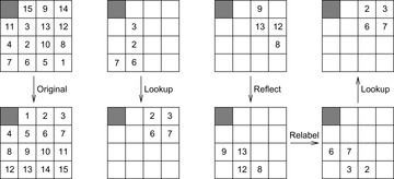
What is needed are symmetries that preserve shortest path information with respect to the abstract goal. Hence, symmetry pattern database lookups exploit physical symmetries of the problem that do exist for the goal state(s). For example, because of the length-preserving symmetry along the main diagonal in the (n² − 1)-Puzzle, the pattern database built for the tiles 2, 3, 6, and 7 can also be used to estimate the number of moves required for patterns 8, 9, 12, and 13 as shown in Figure 4.12. More formally, for a given (n² − 1)-Puzzle with a state

and a symmetry

, the symmetry lookup is executed on state u′ with

, where

and

B9780123725127000043/f04-12-9780123725127.jpg is missing

Figure 4.12

Ordinary (left) and symmetry (right) pattern database lookup tiles are reflected along the main diagonal, relabeled, and queried in the original pattern database for retrieving the exact goal distance.

Another example is the well-known Towers-of-Hanoi problem. It consists of three pegs of different-size discs, which are sorted in decreasing order of size on one of the pegs. A solution has to move all discs from their initial peg to a goal peg, subject to the constraint that a smaller disk is above a larger one. A pattern database symmetry is found by exploiting that the two nongoal pegs are indistinguishable. Note that the three-peg problem is not a challenging combinatorial problem any more because the lower and upper bounds of

moves match by simple arguments on a recursive solution (to build an n tower from peg A to C move the top

tower to B, then the largest disk from A to C, and finally the

tower from B to C). The four-peg Towers-of-Hanoi problem, however, is a search challenge.

A related aspect to symmetry is duality. Dual pattern database lookups require a bijection between objects and locations of the domain in the sense that each object is located in one location and each location occupies only one object. There are three main assumptions: Every state is a permutation, the actions are location-based, and the actions are inversible. An example is provided in Figure 4.13. The dual question is generated by first selecting the goal positions for the tiles that are in the pattern locations (inversion) and then substituting the tiles with their indexes. The dual lookup itself can reuse the database.

B9780123725127000043/f04-13-9780123725127.jpg is missing

Figure 4.13

Ordinary and dual pattern database lookups initial and goal states (far left); ordinary lookup in the pattern database for the tiles 2, 3, 6, and 7 (left, the pattern itself is shown on the top, its respective goal is shown on the bottom). For a dual lookup we generate a dual question (right, top to bottom) followed by a lookup in the pattern database for the tiles 2, 3, 6, and 7 (far right, bottom to top).

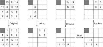
Experimental results show that the average heuristic value increases when using symmetry or duality or both. Symmetry pattern database lookups are used for the same search direction as for the original pattern database lookup, whereas dual lookups result in estimates for backward search.

4.5.3. Bounded Pattern Databases

Most pattern database heuristics assume that a memory-based heuristic is computed for the entire state space, and the cost of computing it is amortized over many problem instances. But in some cases, it may be useful to compute pattern database heuristics for a single problem instance. If we know an upper bound U for the minimum cost solution

in original space S, one option to reduce the memory needs is to limit the exploration in abstract space to a superset of the ones that are relevant for being queried in the concrete state space search. Assume that A* search with cost function f is applied in the backward traversal of the abstract space to guide the search toward the abstract start state

. When terminating at

not all relevant abstract goal distances have been computed. Pattern database construction has to continue according to a different termination criterion. The following simple observation limits the exploration in the focused traversal of abstract space. In other words, goal distances of some particular abstract states can be safely ignored, based on the following result.

Theorem 4.5

(Bounded Computation of Pattern Database) Let U be an upper bound on

, the cost of the optimal solution to the original problem, let ϕ be the state space abstraction function, and let f be the cost function in the backward traversal of the abstract space. A pattern database entry for u only needs to be computed if

Proof

Since the f-value in an abstract state for a state

provides a lower bound on the cost of an optimal solution in abstract space, which in turn is a lower bound on the cost of the optimal solution to the original problem, it follows that for any projected state

of which the f-value exceeds U, it cannot lead to any better solution with cost lower than U and thus can be safely ignored in the computation.

The situation is shown to the left in Figure 4.14, where we see the concrete state space on top of the abstract one. The relevant part that could be queried by the top-level search is shaded. It is contained in the cover

B9780123725127000043/f04-14-9780123725127.jpg is missing

Figure 4.14

Successful one-pass A* pattern database construction (left), and demand for extension of secondary A* search in abstract state space (right). Nodes searched by A* in the original graph and states needed for the database lookup are shaded gray, and nodes searched by A* in the inverse abstract state space graph, (A*)⁻¹ for short, are indicated with an ellipse.

Consequently, A* for pattern database creation terminates when condition

is not satisfied. The following result shows that the technique is particularly useful in computing a set of disjoint pattern database heuristics.

Theorem 4.6

(Bounded Construction of Disjoint Pattern Databases) Let

be the difference between an upper bound U and a lower bound

on the cost of an optimal solution to the original problem, where h is a consistent heuristic and

is the initial state for the abstract problem. A state

for the construction of a disjoint pattern database heuristic needs to be processed only if

Proof

In disjoint pattern database heuristics, the cost of optimal solution to each abstract problem can be added to obtain an admissible heuristic to the original problem. Therefore, it can be shown that a pattern database heuristic needs only to be computed for

. Subsequently, for every abstraction

we have

. Since all heuristics are consistent, we have

. It follows that

Because

, we get

4.5.4. On-Demand Pattern Databases

Another option for reducing the space occupied by the pattern databases is not to apply heuristic backward search in the abstract space. For the sake of simplicity, we assume a problem graph, in which the initial and goal state are unique. In the abstract space the pattern database is constructed backward from the goal using a heuristic that estimates the distance to the abstract initial state. When the initial pattern is reached, pattern construction is suspended. The set of expanded nodes in abstract space can be used for lookups in forward search, as they contain optimal distance values to the goal (assuming a consistent heuristic and maintaining the g-value).

Consider the situation as shown in Figure 4.14. The left part of the figure displays the concrete state space and the mapping of the initial state s and goal state t to their corresponding abstract counterparts. We see that A* executed in the concrete state space and abstract A* executed in the abstract state space do not fully traverse their state spaces. As said, the search in abstract state space is suspended once the goal has been found, and the information computed corresponds to a partially constructed pattern database.

In the best case, all states queried in the concrete search will be mapped to states that have been generated in the abstract state space. To the right in Figure 4.14 we see, however, that the abstract states generated for queries in the original A* (indicated by another ellipse, labeled with A*) can be located outside the states set already generated in an abstract A* search. In this case, heuristic values for the concrete state space have to be computed on demand. The suspended exploration in abstract state space is resumed until the state that has been queried is contained in the enlarged set. Hence, the pattern database grows dynamically (until memory is exhausted).

There is a subtle issue that influences the runtime of the approach. To allow the secondary search to be guided toward the new abstract query states (that failed the lookup procedure), the entire search frontier of the suspended abstract A* search has to be reorganized. Let

be the heuristic for the first and

be the estimator for the subsequent abstract goal, then the priorities in the search frontier have to be changed from

4.5.5. Compressed Pattern Databases

Generally, the larger patterns become, the more powerful the heuristic will be in reducing the search efforts. Unfortunately, due to its size we might reach the physical memory limits of the computer very soon. Therefore, it can be beneficial to consider hash compression techniques to push the limits further.

Compressed pattern databases partition the abstract search space into clusters or groups of nodes. They contribute to the fact that it is possible to generate abstract search spaces beyond the limit of main memory. These spaces are generated but not stored completely, either by omitting the visited set from the search (see Ch. 6), or by maintaining the state space externally on the hard disk (see Ch. 8).

The compression mapping folds the hash table representation of the pattern databases. A group of entries is projected to one representative location and if hash conflicts are detected, the entry stored will be the minimum of all patterns that map to the same address to preserve admissibility. Unfortunately, this induces that the heuristic can drop by more than the edge costs, giving rise to possible inconsistencies.

Theorem 4.7

(Nearby Pattern Database Compression) Assume that for two abstract states

and

we have

. Then

Proof

By applying the triangular inequality for shortest paths

we obtain

As a consequence, if nearby patterns are compressed, the loss of information is bounded. Finding domain-dependent problem projections that preserve the locality in the abstract search graph is a challenge. Hence, one compression technique is based on connected subgraphs that appear in the search space and that are contracted using the projection function. The most prominent examples are cliques, sets of nodes that are fully connected via edges. In this case the entries in the pattern database for these nodes will differ from one another by at most 1. Of course, cliques in pattern space are domain dependent and do not exist in every problem graph. Furthermore, when cliques exist, their usage for compressing the pattern database depends heavily on the index function used. Nonetheless, at least for permutation-type domains, the hope is that cliques will appear quite often.

Suppose that k nodes of the pattern space form a clique. If we can identify a general subgraph structure for k adjacent entries, we can compress the pattern database by contracting it. Instead of storing k entries, we map all nodes in the subgraph to one entry. An admissible compression stores the minimum of the k nodes.

This compression can be generalized and included into pattern database construction as follows. Suppose that we can generate but not fully store an abstract state space. At each abstract state generated, we further map it to a smaller range, and address a pattern database hash table of this compressed index range. As several abstract states now share the same address in the compressed pattern database, we store the smallest distance value. An example is provided in Table 4.4.

**Table 4.4** Compressing a pattern database: original pattern database (left), compressed database (right).
Address	Value	Compressed Address (stored)	Original Address (not stored)	Value (stored)
1	4	1	{1,2}	4
2	5	2	{3,4}	6
3	6	3	{5,6}	3
4	7	4	{7,8}	1
5	5
6	3
7	2
8	1

Viewed differently, such compression is a hash abstraction in the form of an equivalence relation. It clusters nodes with the same hash value, updating costs and using the minimum. There is a tight connection of pattern database compression to other hash compression techniques like bit-state hashing (see Ch. 3).

For the compression, the state space that is traversed is larger than the one that is stored. The search frontier for exploring the entire abstract space has to be maintained space-efficiently, for example, on disk (see Ch. 8).

Traversing the larger abstract state space does pay off. We show that the values in compressed pattern databases are in general significantly better than the ones generated in corresponding uncompressed databases bound by the available memory.

Theorem 4.8

(Performance of Pattern Database Compression) For permutation problems with n variables and a pattern of p variables, let

denote the database heuristic when abstracting k and let

denote the database heuristic when removing k of the p variables. Then the sizes of the pattern databases match and for all states u we have

Proof

Both abstract search spaces contain

states. Whereas ϕ simply ignores the k variables,

takes the minimum value for all possible combinations of the k variables.

4.5.6. Compact Pattern Databases

An alternative for reducing the space requirement for a pattern database is to exploit the representation of a state as a string and a trie implementation for the pattern database. For each pattern, a path in a trie is generated, with the heuristic value at the leaves. This representation is sensible to orderings of characters in the string that describe the pattern, and might be optimized for better space consumption. Leaves of common heuristic values can be merged and isomorphic subtrees can be eliminated. In contrast to the pattern database compression, compaction is lossless, since the accuracy of the pattern database is not affected.

Lastly, there are various compression techniques known from literature (e.g., run-length, Huffman, and Lempel-Ziv) that can be applied to pattern databases to reduce their memory consumption. The core problem with these techniques is that a pattern database (or parts of it) have to be uncompressed to perform a lookup.

4.6. Summary

A* and its variants are more focused if they use heuristic estimates of the goal distances and then find shortest paths potentially much faster than when using the uninformed zero heuristics. In this chapter, we therefore discussed different ways of obtaining such informed heuristics, which is often done by hand but can be automated to some degree.

Abstractions, which simplify search problems, are the key to the design of informed heuristics. The exact goal distances of the abstract search problem can be used as consistent heuristics for the original search problem. Computing the goal distances of the abstract search problem on demand does not reduce the number of expanded states, and the goal distances just need to be memorized. The goal distances of several abstractions can be combined to yield more informed heuristics for the original search problem. Abstractions can also be used hierarchically by abstracting the abstract search problem further. Most consistent heuristics designed by humans for some search problem turn out to be the exact goal distances for an abstract version of the same search problem, which was obtained either by adding actions (embeddings) or grouping states into abstract states. Embeddings, for example, can be obtained by dropping preconditions of operators, whereas groupings can be obtained by clustering close-by states, dropping predicates from the STRIPS representations of states, or replacing predicates with don't care symbols independent of their parameters (resulting in so-called patterns). This insight allows us to derive consistent heuristics automatically by solving abstract versions of search problems.

We discussed a negative speed-up result for embeddings: Assume that one version of A* solves a search problem using the zero heuristics. Assume further that a different version of A* solves the same search problem using more informed heuristics that, if needed, are obtained by determining the goal distances for an embedding of the search problem with A* using the zero heuristics. Then, we showed that the second scheme expands at least all states that the first scheme expands and thus cannot find shortest paths faster than the first scheme. This result does not apply to groupings but implies that embeddings are helpful only if the resulting heuristics are used to solve more than one search problem or if they are used to solve a single search problem with search methods different from the standard version of A*.

We discussed two ways of obtaining heuristics by grouping states into abstract states. First, Hierarchical A* calculates the heuristics on demand. Hierarchical A* solves a search problem using informed heuristics that, if needed, are obtained by determining the goal distances for a grouping of the search problem with A* that can either use the zero heuristics or heuristics that, if needed, are obtained by determining the goal distances for a further grouping of the search problem. The heuristics, once calculated, are memorized together with the paths found so that they can be reused. Second, pattern databases store in a lookup table a priori calculated heuristics for abstract states of a grouping that typically correspond to the smallest goal distances in the original state space of any state that belongs to the abstract states.

Pattern databases result in the most powerful heuristics currently known for many search problems. We discussed Korf's conjecture that the number of states generated by A* (without duplicate detection) using a pattern database is approximately proportional to the ratio of the number of states in the state space and the size of the pattern database. Instead of using one large pattern database, we can often obtain more informed consistent heuristics by using several smaller pattern databases and taking the maximum or, if each operator application is counted in at most one of the pattern databases (resulting in so-called disjoint pattern databases), the sum of their heuristics. Sometimes we can also obtain more informed consistent heuristics from a plain pattern database by exploiting symmetry and duality, a special form of symmetry. We can design good pattern databases by hand or automatically compute the heuristics stored in the pattern database for all abstract states or only a superset of the relevant ones (if we know an upper bound on the length of the shortest path), compute these heuristics a priori or on demand, store these heuristics in a compressed or uncompressed form, and choose statically or dynamically which pattern databases to combine to guarantee that the pattern databases are disjoint.

Table 4.5 summarizes different ways of constructing pattern databases, where k is the number of (not necessarily disjoint) patterns and l is the number of disjoint patterns. Then we list the search methods used in the forward and backward search directions separately. A dash denotes that an (additional) search in the given direction is not needed, and an asterisk denotes that any search method can be used. User lists the information provided by the designer of the pattern database. Lookup lists the number of heuristics retrieved from the pattern database to calculate the heuristic of one state. Admissible lists the condition under which the resulting heuristics are admissible. A checkmark denotes that they are guaranteed to be admissible in any case, otherwise it is shown how the heuristics of several pattern databases need to be combined to guarantee admissibility.

**Table 4.5** Overview pattern databases: ϕ is a state space abstraction, ψ a state space partition; maxMem denotes the use of automated pattern selection with regard to pattern database size threshold, and U denotes an upper bound on the length of the shortest path for the search problem in the original state space. Notation √ ⇒ √ is ad hoc for saying that if the pattern database heuristic is admissible then the dual is admissible as well.
Pattern Database	Forward	Backward	User	Lookup	Admissible
Ordinary	-	BFS	ϕ	1	√
Directed	Any	BFS	ϕ	1	√
Weighted	Any	Dijkstra	ϕ	1	√
Multiple	k×Any	k×*	ϕ_i, maxMem	k	max
Disjoint	l×Any	l×*	ϕ_i, maxMem	l	add
Multiple Disjoint	kl×Any	kl×*	ϕ_i, maxMem	kl	add/max
Bounded	-	BFS	ϕ,U	1	√
On-Demand	-	A*	ϕ	1	√
Symmetry	-	-	ϕ, Symmetry	s	√
Dual	-	-	ϕ, Duality	2	√ ⇒ √
Compressed	-	BFS	ϕ, ψ	1	√

4.7. Exercises

4.1 Consider the Fifteen-Puzzle with all labels of the tiles removed. Display the abstract state space and annotate the distances to the goal.

4.2 The Thirty-Five-Puzzle is the n = 6 variant of the (n² − 1)-Puzzle.

1. Determine the sizes of the abstract state spaces for a growing number of tiles in the pattern.

2. Assuming a perfect hash table with one byte per entry, estimate the amount of memory needed for a disjoint set of 6-tile and a disjoint set of 7-tile pattern databases.

4.3 Provide a sufficient condition for the inversion of an operator in PSVN.

4.4 The Arrow Puzzle asks for changing the order of the arrows in an arrangement, while flipping two adjacent arrows at a time.

1. Transform the initial state

into

2. Devise an abstraction by solving any 4-Arrow Puzzle subproblem. How many subproblems do you obtain?

3. Illustrate that the solution length reduces linearly, but the state space reduces exponentially.

4.5 Consider the three-disk Towers-of-Hanoi Puzzle with the disks small, middle, and big and three pegs.

1. Depict the entire state space (level 0). How many states does it have?

2. Depict the entire state space for the problem where only the middle and smallest disk are provided (level 1). How many states does it have?

3. Depict the entire state space for the problem where only the smallest disk is provided (level 2). How many states does it have?

4. Show levels 0, 1, and 2 of the abstraction hierarchy formed for the initial state.

4.6 In a Blocksworld problem involving n blocks b_i it is possible to define n patterns and relaxations as follows. The variables pos(b_i) encode the position of block b_i. The value pos(b_i) is 0 if b_i is located on the table and j if it is located on another block b_j, j ≠ i.

1. Show that such patterns are disjoint; that is, no action affects more than one variable.

2. For all blocks that are on the table to build an n-tower show that an according pattern database heuristic results in the value n.

3. For an n-tower, where only the two bottom-most blocks are to be exchanged, show that the preceding pattern database heuristic results in the value 1.

4.7 For the Fifteen-Puzzle instance (14, 13, 15, 7, 11, 12, 9, 5, 6, 0, 2, 1, 4,8) compute the disjoint pattern database value with respect to the goal state and

1. one tile in each pattern. What is the name of the heuristic?

2. two tiles in each pattern; that is, group the tiles (1,2), (1,3), …, (14,15).

4.8 Consider the disjoint 6-tile pattern databases in Figure 4.7.

1. Validate that the maximal depth of the regular 6-pattern databases is 35 and explain why the construction of only one of the three pattern databases is sufficient.

2. The irregular 6-tile pattern database encloses the blank, which limits the last two moves of the tiles (e.g., the last tile that can move is either tile 1 or tile 5 for the standard layout of the puzzle). How far does this technique increase the initial maximal depth of 32? Does this affect the consistency of the database? Why or why not?

4.9 Explain how to construct a pattern database if the abstract state space contains more than one abstract goal state.

4.10 Show that

1. max{h₁, h₂} induced by ϕ₁ and ϕ₂ dominates h₁ and h₂.

2. h₁ + h₂ induced by disjoint ϕ₁ and ϕ₂ dominates h₁ and h₂.

for

generated by unifying ϕ₁, ϕ₂ dominates both max{h₁, h₂} and h₁ + h₂.

4. h^C dominates all h_i, induced by ϕ_i,

4.11 Explain why in Sokoban we have used the minimum weighted matching, but in the sliding-tile puzzle we have used the maximum weighted matching to combine the subproblems.

4.12 For the 2 × 2 version of the (n² − 1)-Puzzle:

1. Display the concrete and the abstract state spaces generated by mapping all labels to 1.

2. Show that introducing two blanks leads to spurious states that have no concretization.

3. Give a general characterization that no spurious state is generated.

4.13 Consider the 4×4 Gridworld with initial state at the bottom-left and the goal state at the top-right corner. Additionally, insert edges along the diagonal, and connect (i, i) with (i+1, i+1) for all available values of i by undirected edges. Let h_r denote the row distance of a node to the goal and h_c the column distance.

1. Perform BFS on the problem.

2. Show that using either h_r or h_c alone reduces the amount of search by a factor of two.

3. Show that maximizing the two heuristics leads to a search that proceeds directly down the optimal solution path along the diagonal edges.

4.14 Consider a Fifteen-Puzzle instance

1. Determine the abstract goal distances for the two pattern tile selections (1,2,4,5,6,8,9,10) and (3,7,11,12,13,14,15) by counting each move in abstract space. Maximize the values to compute an admissible heuristic estimate.

2. Determine the abstract goal distances for the two pattern tile selections (1,2,3,4,5,6,7) and (8,9,10,11,12,13,14,15) counting each pattern tile move in abstract space. Add the values to compute an admissible heuristic.

4.15 Given a weighted graph, the Sequential Ordering problem asks for a minimal-cost Hamiltonian path from the start node to the goal vertex, which also observes precedence constraints. An instance to the problem can be defined by a cost matrix, where the entry is the cost of the edge, or it is −1 to represent that the first node must precede the second node in the solution path. A state corresponds to a partial completion of the trip. It records the current last vertex in this partial tour as well as the nodes that have not been reached yet.

1. Provide a representation of a state space in the form of a lattice with the start state at the top and the goal state at the bottom. Your lattice should have as many layers as there are nodes in the graph. Draw an example problem with three nodes.

2. Construct an abstract state space lattice with the same number of levels but with a lesser number of states. The abstract lattice should be obtained by clustering states on the same level. In your chosen example you should merge nodes 1 and 3 in level 1, and nodes 1 and 2 in levels 2 and 3. Show the outcome of the abstraction.

3. Describe the modifications to the cost matrix and prove that the abstraction is a lower bound.

4.16 Explain why maximizing of two heuristics can fail to produce better search results than one of the individual exploration. Hint: Use the odd/even parity of the f-value in the (n² − 1)-Puzzle.

4.17 For the Eight-Puzzle use the domain abstractions ϕ₁, which maps the vector of tiles (1, 2, 3, 4, 5, 6, 7, 8, 0) to the vector (x, x, 3, 4, 5, 6, x, 8, 0), and ϕ₂, which maps (1, 2, 3, 4, 5, 6, 7, 8, 0) to (x, x, y, y, 5, z, x, z, 0).

1. Determine the sizes of the abstract space generated by ϕ₁ and ϕ₂.

2. Why can it be better to map values to more than one don't care symbol?

4.18 The granularity of a domain abstraction is a vector indicating how many constants in the original domain are mapped to each constant in the abstract domain. For example, the granularity of ϕ₂ in Exercise 4.17 is (3,2,2,1,1) because three constants are mapped to x, two are mapped to y, two are mapped to z, and constants 5 and 0 remain unique.

1. Determine the granularity of ϕ₁.

2. Determine the expected sizes of the abstract spaces for the Eight-Puzzle based on the granularity (3, 3, 2, 1) by first determining n, the number of different domain abstractions with this granularity, and m, the pattern space size for each of the abstractions.

3. Provide an Eight-Puzzle example that shows that different granularities can produce pattern state space of the same size.

4.19 Graph abstractions ensure that if there is an initial goal path in the concrete cost-algebraic graph, there is one in the abstract system, and that the cost of the optimal initial goal path in the concrete system is smaller (w.r.t.

) than the cost of the one in the abstract system.

1. Illustrate the merging of nodes v₁, v₂ in a (multiple-edge) graph with edges

, and

2. Show that merging nodes to super-nodes leads to a graph abstraction.

3. Show how merging of edges reduces the search effort.

4. Show that self-loops can be eliminated because they do not contribute to a better solution.

4.20 Rubik's Cube (see Ch. 1) is one of the best examples to apply symmetries. The cube has 48 symmetries including reflections. Show that these symmetries can be generated by four basic symmetries.

4.21 Let us now look at conjugation for the Rubik's Cube, a fundamental concept in group theory. For example, the operation

twists two specific corners on a face. For any element h in the cube group,

will twist some pair of corners. Repeating the conjugate operation n times yields

1. Show that conjugacy, as defined for the Rubik's Cube, is an equivalence relation.

2. Enumerate the conjugacy classes of S₄.

3. Consider the Rubik's Cube and apply the commutator

and the conjugated commutator

. Display your result!

4. Now raise conjugation to a power,

, and so on.

4.22 If you turn the faces of a solved cube and do not use the moves R, R⁻¹, L, L⁻¹, F, F⁻¹, B, and B⁻¹, you will only generate a subset of all possible cubes. This subset is denoted by

. In this subset, the orientations of the corners and edges cannot be changed and the four edges in the UD-slice (between the U-face and D-face) stay isolated.

1. Show that mapping a concrete cube position to one in G₁ is a state space abstraction.

2. How many states are contained in G₁?

3. Determine the goal distances in G₁ using backward BFS.

4. Devise a two-phase algorithm that first searches for the shortest path for any state to one in G₁ and that then searches for the shortest path within G₁. Is this strategy optimal (i.e., does it yield optimal solutions)?

4.8. Bibliographic Notes

Using abstraction transformations to guide the search goes back to Minski who defined abstractions as the unification of a simplified problem and refinement in the early 1960s. The ABSTRIPS solver technology is due to Sacerdoti (1997). The history on automated creation of admissible heuristics ranges from early work of Gaschnig (1979b), Pearl (1985) and Preditis (1993), to Guida and Somalvico (1979). Gaschnig has proposed that the cost of solutions can be computed by exact solution in auxiliary space. He observed that search with abstract information can be more time consuming than breadth-first search. Valtorta (1984) has proven this conjecture and published a seminal paper, which has been reconsidered by Holte, Perez, Zimmer, and Donald (1996). An update on Valtorta's result is due to Hansson, Mayer, and Valtorta (1992). Hierarchical A* has been revisited by Holte, Grajkowski, and Tanner (2005). The authors have also invented hierarchical IDA*. Absolver by Mostow and Prieditis (1989) was the first system to break the barrier imposed by the theorems. They implemented the idea of searching through the space of abstractions and speed-up transformations. In later research, one of the authors suggests to store all heuristic values before base-level search in a hash table.

Pattern databases have been introduced by Culberson and Schaeffer (1998) in the context of the Fifteen-Puzzle. The name refers to (don't care) pattens as abstractions. This suggests to revise the name to abstraction databases since any abstraction (based on patterns or not) can be used. Despite such attempts, for example by Qian (2006), in AI research the term pattern database has settled. They have shown to be very effective in solving random instances of the Rubik's Cube by Korf (1997) and the Twenty-Four-Puzzle by Korf and Felner (2002) optimally. Holte and Hernádvölgyi (1999) have given a time-space trade for pattern database search (Korf, Reid, and Edelkamp, 2001). Additive pattern databases have been proposed by Felner, Korf, and Hanan (2004a) and general theory on additive state space abstraction has been given by Yang, Culberson, Holte, Zahavi, and Felner (2008). Edelkamp (2002) has shown how to construct pattern databases symbolically. Hernádvölgyi (2000) has applied pattern databases to significantly shorten the length of macro actions.

Multiple pattern databases have been studied by Furcy, Felner, Holte, Meshulam, and Newton (2004) in the context of puzzle solving. The authors also discuss limits and possibilities of different pattern partitions. Breyer and Korf (2010a) have shown that independent additive heuristics reduce search multiplicatively. Zhou and Hansen (2004b) have analyzed a compact space-efficient representation of pattern databases. Multivalued pattern databases are variants of multiple goal pattern databases that improve the performance of single-valued pattern databases in practice, and have been suggested by Linares López (2008) and vectorial pattern databases, as proposed by Linares López (2010), induce nonconsistent heuristic functions by recognizing admissible heuristic values.

Machine learning methods for multiple pattern database search, including their selection and compression, are discussed by Samadi, Felner, and Schaeffer (2008a) and by Samadi, Siabani, Holte, and Felner (2008b). Symmetric pattern databases have already been considered by Culberson and Schaeffer (1998). Lookups based on the duality of positions and state vector elements have been studied by Felner, Zahavi, Schaeffer, and Holte (2005). In Zahavi, Felner, Holte, and Schaeffer (2008b) general notions of duality are discussed, but are limited to location-based permutations. On-demand or instance-dependent pattern databases have been introduced by Felner and Alder (2005) and compressed databases are due to Felner, Meshulam, Holte, and Korf (2004b). Bitvector pattern databases based on two-bit BFS are proposed by Breyer and Korf (2010b). A method for learning good compression has been suggested by Samadi et al. (2008b). For large range of planning domains, Ball and Holte (2008) have shown that BDD sometimes achieve very large compression ratios. A first theoretical study on BDD growth in state space search has been provided by Edelkamp and Kissmann (2008c). Counterintuitively, inconsistencies (e.g., due to random selection of pattern databases) positively reduce search efforts, see work by (Zahavi, Felner, Schaeffer, and Sturtevant, 2007). Applying machine learning for bootstrapping has been proposed by Jabbari, Zilles, and Holte (2010).

The interrelation of abstraction and heuristics has been emphasized by Larsen, Burns, Ruml, andHolte (2010). Neccessary and sufficient conditions for avoiding spurious states have been studied by Zilles and Holte (2010) and abstraction-based heuristics with true distance heuristics have been considered by Felner and Sturtevant (2009) as a way to obtain admissible heuristics for explicit state spaces. In a variant, called portal heuristic, the domain is partitioned into regions and portals between regions are identified. True distances between all pairs of portals are stored and used to obtain admissible heuristics for A* search.

The application of pattern databases are manifold. The multiple sequence alignment problem as introduced in Chapter 1 calls for sets of n sequences to be optimally aligned with respect to some similarity measurement. The heuristic estimates as applied in Korf and Zhang (2000); McNaughton, Lu, Schaeffer, and Szafron (2002); and Zhou and Hansen (2004b) is to find and add the lookup values of alignments of disjoint subsets for

sequences. Pattern databases together with A* have been applied by Klein and Manning (2003) to find the best parsing of a sentence. The estimate correlates to the cost of completing a partial parse and is derived by simplifying the grammar. Finding a least-cost path in quality-of-service routing problems (see Ch. 2) has been considered by Li, Harms, and Holte (2007) with different estimate functions for each of the resources. Each estimate is derived by considering only the constraint on the considered resource. The approach relates to finding the shortest path subject to multiple constraints by Li, Harms, and Holte (2005).

The Sequential Ordering problem has been analyzed by Hernádvölgyi (2003) using pattern databases. Another application area for pattern databases is interactive entertainment. For cooperative plan finding in computer games many agents search for individual paths but are allowed to help each other to succeed. Silver (2005) has shown how to incorporate memory-based heuristics. In constraint optimization, bucket elimination as proposed by Kask and Dechter (1999) shares similarities with pattern databases, providing an optimistic bound on the solution cost.

Knoblock (1994) has found that techniques that drop a predicate entirely from a state space in domain-independent action planning are homomorphisms. Haslum, Bonet, and Geffner (2005) have discussed the automated selection of pattern databases in the context of optimal planning. The paper extends the work of Edelkamp (2001a), who has applied pattern database search to AI planning (see Ch. 15).

Abstraction is a fundamental concept in the area of model checking(Clarke, Grumberg, and Long, 1994). Cleaveland, Iyer, and Yankelevich (1995) have presented an alternative setting. The concept of path preservation is called simulation and has been explained by Milner (1995). Merino, del Mar Gallardo, Martinez, and Pimentel (2004) have presented a tool to perform data abstraction for the verification of communication protocols. Predicate abstraction is a related abstraction method that is important to control the branching in software programs and has been introduced by S. Graf and H. Saidi (1997). It is the basis of the counterexample-guided abstract-and-refinement paradigm, invented by Clarke, Grumberg, Jha, Lu, and Veith (2001) and integrated in state-of-the-art tools, for example, by Ball, Majumdar, Millstein, and Rajamani (2001). The first applications of pattern databases in verification are due to Qian and Nymeyer (2004) and Edelkamp and Lluch-Lafuente (2004).

..................Content has been hidden....................

You can't read the all page of ebook, please click here login for view all page.

Table of Contents for Chapter 4. Automatically Created Heuristics

Create new playlist

Sign In

Sign Up

4.1. Abstraction Transformations

4.2. Valtorta's Theorem

4.3. *Hierarchical A*

4.4. Pattern Databases

4.4.1. Fifteen-Puzzle

4.4.2. Rubik's Cube

4.4.3. Directed Search Graphs

4.4.4. Korf's Conjecture

4.4.5. Multiple Pattern Databases

4.4.6. Disjoint Pattern Databases

4.5. * Customized Pattern Databases

4.5.1. Pattern Selection

4.5.2. Symmetry and Dual Pattern Databases

4.5.3. Bounded Pattern Databases

4.5.4. On-Demand Pattern Databases

4.5.5. Compressed Pattern Databases

4.5.6. Compact Pattern Databases

4.6. Summary

4.7. Exercises

4.8. Bibliographic Notes

Table of Contents for
Chapter 4. Automatically Created Heuristics

4.3. Hierarchical A