
Chapter 16. Automated System Verification
This chapter gives a general introduction to search problems in model checking, Petri nets, and graph transition systems. It also gives a general introduction to automated theorem proving and discusses state space search for proof state–based theorem proving and diagnosis problems.
Keywords: verification, validation, model checking, temporal logic, communication protocol, directed model checking, trail-directed search, program model checking, Petri net, real-time system, timed automaton, priced timed automaton, graph transition system, knowledge base anomaly, diagnosis, general diagnostic engine, automated theorem proving
The presence of a vast number of computing devices in our environment imposes a challenge for designers to produce reliable software. In medicine, aviation, finance, transportation, space technology, and communication, we are more and more aware of the critical role correct hardware and software plays. Failure leads to financial and commercial disaster, human suffering, and fatalities. However, systems are harder to verify than in earlier days. Testing if a system works as intended becomes increasingly difficult. Nowadays, design groups spend 50% to 70% of the design time on verification. The cost of the late discovery of bugs is enormous, justifying the fact that, for a typical microprocessor design project, up to half of the overall resources spent are devoted to its verification. In this chapter we give evidence of the important role of heuristic search in this context.
The process of fully automated property verification is referred to as model checking and will cover most of the presentation here. Given a formal model of a system and a property specification in some form of temporal logic, the task is to validate whether or not the specification is satisfied in the model. If not, a model checker returns a counterexample for the system's flawed behavior helping the system designer to debug the system. The major disadvantage of model checking is that it scales poorly; for a complete verification each state has to be looked at. With the integration of heuristics into the search process (known as directed model checking) we look at various options for improved search. The applications range from checking models of communication protocols, Petri nets, real-time as well as graph transition systems, to the verification of real software. We emphasize the tight connection between model checking and action planning.
Another aspect of automated system verification that is especially important for AI applications is to check whether or not a knowledge-based system is consistent or contains anomalies. We address how symbolic search techniques can be of help here. We give examples of symbolic search in solving (multiple-fault) diagnosis problems.
Most of the work in heuristic search for automated system verification concentrates on accelerated falsification. With directed automated theorem proving, algorithms like A* and greedy best-first search are integrated in a deductive system. As theorem provers draw inferences on top of axioms of an underlying logic, the state space is the set of proof trees. More precisely, sets of clauses for a proof state are represented in the form of a finite tree and rules describe how a clause is obtained by manipulating a finite set of other input clauses. Inference steps are performed mainly via resolution. Since such systems are provided in functional programming languages, we look at functional implementations of search algorithms.
16.1. Model Checking
Model checking has evolved into one of the most successful verification techniques. Examples range from mainstream applications such as protocol validation, software checking, and embedded system verification, to exotic areas such as business work-flow analysis and scheduler synthesis. The success of model checking is largely based on its ability to efficiently locate errors. If an error is found, a model checker produces a counterexample that shows how the errors occur, which greatly facilitates debugging. In general, counterexamples are executions of the system, which can be paths (if linear logics are used) or trees (if branching logics are used).
However, while current model checkers find error states efficiently, the counterexamples are often unnecessarily complex, which hampers error explanation. This is due to the use of naive search algorithms.
There are two primary approaches to model checking. First, symbolic model checking applies a symbolic representation for the state set, usually based on binary decision diagrams. Property validation in symbolic model checking amounts to some form of symbolic fixpoint computation. Explicit-state model checking uses an explicit representation of the system's global state graph, usually given by a state transition function. An explicit-state model checker evaluates the validity of the temporal properties over the model, and property validation amounts to a partial or full exploration of a certain state space. The success of model checking lies in its potential for push-button automation and in its error reporting capabilities. A model checker performs an automated complete exploration of the state space of a software model, usually using a depth-first search strategy. When a property violating a state is encountered the search stack contains an error trail that leads from an initial system state into the encountered state. This error trail greatly helps software engineers in interpreting validation results.
The sheer size of the reachable state space of realistic software models imposes tremendous challenges on model checking technology. Full exploration of the state space is often impossible, and approximations are needed. Also, the error trails reported by depth-first search model checkers are often exceedingly lengthy—in many cases they consist of multiple thousands of computation steps, which greatly hampers error interpretation.
In the design process of systems two phases are distinguished. In a first explanatory phase, we want to locate errors fast; in a second fault-finding phase, we look for short error trails. Since the requirements of the two phases are not the same, different strategies apply. In safety property checking the idea is to use state evaluation functions to guide the state space exploration into a property violating state. Greedy best-first search is one of the most promising candidate for the first phase, but yield no optimal solution counterexamples. For the second phase, the A* algorithm has been applied with success. It delivers optimally short error trails if the heuristic estimate for the path length to the error trail is admissible. Even in cases where this cannot be guaranteed, A* delivers very good results.
The use of heuristic search renders erstwhile unanalyzable problems to ones that are analyzable for many instances. The quality of the results obtained with A* depends on the quality of the heuristic estimate, and heuristic estimates were devised that are specific for the validation of concurrent software, such as specific estimates for reaching deadlock states and invariant violations.
16.1.1. Temporal Logics
Models with propositionally labeled states can be described in terms of Kripke structures. More formally, a Kripke structure is a quadruple  , where S is a set of states, R is the transition relation between states using one of the enabled operators, I is the set of initial states, and
  is a state labeling function. This formulation is close to the definition of a state space problem in Chapter 1 up to the absence of terminal states. That I may contain more than one start state helps to model some uncertainty in the system. In fact, by considering the set of possible states as one belief state set, this form of uncertainty can be compiled away.
For model checking, the desired property of the system is to be specified in some form of temporal logic. We already introduced linear temporal logic (LTL) in Chapter 13. Given a Kripke structure and a temporal formula f, the model checking problem is to find the set of states in M that satisfy f, and check whether the set of initial states belongs to this state set. We shortly write  in this case.
The model checking problem is solved by searching the state space of the system. Ideally, the verification is completely automatic. The main challenge is the state explosion problem. The problem occurs in systems with many components that can interact with each other, so that the number of global states can be enormous. We observe that any propositional planning problem can be modeled as an LTL model checking problem as any propositional goal g can be expressed in the form of a counterexample to the temporal formula  in LTL. If the problem is solvable, the LTL model checker will return a counterexample, which manifests a solution for the planning problem.
The inverse is also often true. Several model checking problems can be modeled as state space problems. In fact, the class of model checking problems that fit into the representation of a state space problem with a simple predicate should be evaluated at each individual state. Such problems are called safety properties. The intuition behind such a property is to say that something bad should not happen. In contrast, liveness properties refer to infinite runs with (lasso-shaped) counterexamples. The intuition is to say that something good will eventually occur.
In automata-based model checking the model and the specification are both transformed into automata for accepting infinite words. Such automata look like ordinary automata but accept if during the simulation of an infinite word one accepting state is visited infinitely often. This assumes that a system can be modeled by an automaton, which is possible when casting all states in the underlying Kripke structure for the model as being accepting. Any LTL formula can be transformed into an automata over infinite words even if this construction may be exponential in the size of the formula. Checking correctness is reduced to checking language emptiness. More formally, the model checking procedure validates that a model represented by an automaton M satisfies its specification represented by an automaton  . The task is to verify if the language induced by the model is included in the language induced by the specification,
  for short. We have
  if and only if
 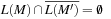 . In practice, checking language emptiness is more efficient than checking language inclusion. Moreover, we often construct the property automaton N for negation of the LTL formula, avoiding the posterior complementation of the automaton over infinite words. The property automaton is nondeterministic, such that both the model and the formula introduce branching to the search process.
16.1.2. The Role of Heuristics
Heuristics are evaluation functions that order the set of states to be explored, such that the states that are closer to the goal are considered first. Most search heuristics are state-to-goal distance estimates that are based on solving simplifications or abstractions of the overall search problems. Such heuristics are computed either offline, prior to the search in the concrete state space, or online for each encountered state (set). In a more general setting, heuristics are evaluation functions on generating paths rather than on states only.
The design of bug hunting estimates heavily depends on the type of error that is searched for. Example error classes for safety properties are system deadlocks, assertion or invariance violations. To guide the search, the error description is analyzed and evaluated for each state. In trail-directed search we search for a short counterexample for a particular error state that has been generated, for example, by simulating the system.
Abstractions often refer to relaxations of the model. If the abstraction is an overapproximation (each behavior in the abstract space has a corresponding one in the concrete space, which we will assume here), then a correctness proof for the specification in the abstract space implies the correctness in the concrete space.
Abstraction and heuristics are two sides of the same medal. Heuristics correspond to exact distances in some abstract search space. This leads to the general approach of abstraction-directed model checking (see Fig. 16.1). The model under verification is abstracted into some abstract model checking problem. If the property holds, then the model checker returns true. If not, in a directed model checking attempt the same abstraction can be used to guide the search in the concrete state space to falsify the property. If the property does not hold, a counterexample can be returned, and if it does hold, the property has been verified.
 |
| Figure 16.1 |
This framework does not include recursion as in counterexample-guided error refinement, a process illustrated in Figure 16.2. If the abstraction (heuristic) turns out to be too coarse, it is possible to iterate the process with a better one.

16.2. Communication Protocols
Communication protocols are examples for finite reactive concurrent asynchronous systems that are applied to organize the communication in computer networks. One important representative of this class is TCP/IP, which organizes the information exchange in the Internet. Control and data flows are essential for communication protocols and are organized either by access to global/shared variables or via communication queues, which are basically FIFO channels. Guards are Boolean predicates associated with each transition and determine whether or not it can be executed. Boolean predicates over variables are conditions on arithmetic expressions, while predicates over queues are either static (e.g., capacity, length) or dynamic (e.g., full, empty). Boolean predicates can be combined via ordinary Boolean operations to organize the flow of control.
In the following we introduce search heuristics used in the analysis of (safety properties for) communication protocols, mainly to detect deadlocks and violations of system invariants or assertions.
16.2.1. Formula-Based Heuristic
System invariants are Boolean predicates that hold in every global system state u. When searching for invariant violations it is helpful to estimate the number of system transitions until a state is reached where the invariant is violated. For a given formula f, let  be an estimate of the number of transitions required until a state v is reached where f holds, starting from state u. Similarly, let
  denote the heuristic for the number of transitions necessary until f is violated.
In Figure 16.3, we illustrate a recursive definition of  as a function of f. In the definition of
  for
for  the use of addition suggests that
  and
and  are independent, which may not be true. Consequently, the estimate is not a lower bound, affecting the optimality of algorithms like A*. If the aim is to obtain short but not necessarily optimal paths, we may tolerate inadmissibilities; otherwise, we may replace addition by maximization.
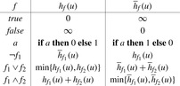 |
| Figure 16.3 |
Formulas describing system invariants may contain other terms, such as relational operators and Boolean functions over queues. We extend the definition of  and
and  as shown in Figure 16.4.
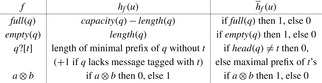
Note that the estimate is coarse but nevertheless very effective in practice. It is possible to refine these definitions for specific cases. For instance,  can be defined as
  in case
  and a is only ever decremented and b is only ever incremented.
The control state predicate definition is given in Figure 16.5. The distance matrix  can be computed with the All Pairs Shortest Paths algorithm of Floyd and Warshall in cubic time (see Ch. 2).
| Figure 16.5 |
The statement assert extends the model with logical assertions. Given that an assertion a labels a transition  , with
  , then we say a is violated if the formula
  is satisfied.
16.2.2. Activeness Heuristic
In concurrent systems, a deadlock occurs if at least a subset of processes and resources is in a cyclic wait situation. State u is a deadlock if there is no outgoing transition from u to a successor state v and at least one end state of a process of the system is not valid. A local control state can be labeled as end to indicate that it is valid; that is, that the system may terminate if the process is in that state.
Some statements are always executable; among others, assignments, else statements, and run statements used to start processes. Other statements, such as send or receive operations or statements that involve the evaluation of a guard, depend on the current state of the system. For example, a send operation q!m is only executable if the queue q is not full, indicated by the predicate  . Asynchronous untagged receive operations (q?x, with x variable) are not executable if the queue is empty; the corresponding formula is ¬empty
  . Asynchronous tagged receive operations (q?t, with t tag) are not executable if the head of the queue is a message tagged with a tag different from t; yielding the formula
  . Moreover, conditions are not executable if the value of the condition corresponding to the term c is false.
The Boolean function executable, ranging over tuples of statements and global system states, is summarized for asynchronous operations and Boolean conditions in Figure 16.6.
 |
| Figure 16.6 |
To estimate the smallest number of transitions from the current state to a deadlock state, we observe that in a deadlock state all processes are necessarily blocked. Hence, the active process heuristics use the number of active or nonblocked processes in a given state: where
where  is defined as
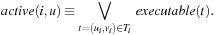 Assuming that the range of
  is contained in
  , the active processes heuristic is not very informative for protocols involving a small number of processes.
Deadlocks are global system states in which no progress is possible. Obviously, in a deadlock state each process is blocked in a local state that does not possess an enabled transition. It is not trivial to define a logical predicate that characterizes a state as a deadlock state that could at the same time be used as an input to the estimation function  . We first explain what it means for a process
  to be blocked in its local state
  . This can be expressed by the predicate blockedi, which states that the program counter of process
  must be equal to
  and that no outgoing transition t from state
  is executable:
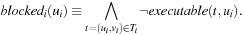 Suppose we are able to identify those local states in which a process i can block; that is, in which it can perform a potentially blocking operation. Let
  be the set of potentially blocking states within process i. A process is blocked if its control resides in some of the local states contained in
  . Hence, we define a predicate for determining whether a process
  is blocked in a global state u as the disjunction of
  for every local state c contained in
  :
: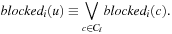 Deadlocks, however, are global states in which every process is blocked. Hence, the disjunction of
  for every process
  yields a formula that establishes whether a global state u is a deadlock state or not:
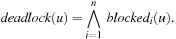 Now we address the problem of identifying those local states in which a process can block. We call these states dangerous. A local state is dangerous if every outgoing local transition can block. Note that some transitions are always executable, for example, those corresponding to assignments. To the contrary, conditional statements and communication operations are not always executable. Consequently, a local state that has only potentially nonexecutable transitions should be classified as dangerous. Additionally, we may allow the protocol designer to identify states as dangerous. Chaining backward from these states, local distances to critical program counterlocations can be computed in linear time.
The deadlock characterization formula deadlock is constructed before the verification starts and is used during the search by applying the estimate  , with f being a deadlock. Due to the first conjunction of the formula, estimating the distance to a deadlock state is done by summing the estimated distances for blocking each process separately. This assumes that the behavior of processes is entirely independent and obviously leads to a nonoptimistic estimate. We estimate the number of transitions required for blocking a process by taking the minimum estimated distance for a process to reach a local dangerous state and negate the enabledness of each outgoing transition in that state. This could lead again to a nonadmissible estimate, since we are assuming that the transitions performed to reach the dangerous state have no effect on disabling the outgoing transitions of that state.
It should be noted that deadlock characterizes many deadlock states that are never reached by the system. Consider two processes  having local dangerous states
  , respectively. Assume that u has an outgoing transition for which the enabledness condition is the negation of the enabledness condition for the outgoing transition from v. In this particular case it is impossible to have a deadlock in which
  is blocked in local state u and
  is blocked in local state v, since either one of the two transitions must be executable. As a consequence the estimate could prefer states unlikely to lead to deadlocks. Another concern is the size of the resulting formula.
16.2.3. Trail-Directed Heuristics
We describe now two heuristics that exploit the information of an already established error state. The first heuristic is designed to focus at exactly the state that was found in the error trail, while the second heuristic focuses on equivalent error states.
Hamming Distance
Let u be a global state given in a suitable binary vector encoding, as a vector  . Further on, let v be the error state we are searching for. One estimate for the number of transitions necessary to get from u to v is called the Hamming distance
  that is defined as:
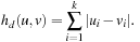 Obviously, in a binary encoding,
  for all
  . Obviously, computing
  is available in time linear in the size of the (binary) encoding of a state. The heuristic is not admissible, since one transition might change more than one position in the state vector at a time. Nevertheless, the Hamming distance reveals a valuable ordering of the states according to their goal distances.
FSM Distance
Another distance metric centers around the local states of component processes. The FSM heuristic is the sum of the goal distances for each local process  ,
,  . Let
. Let  be the program counter of state u in process i. Moreover, let
  be the shortest path distance between the program counters
  and
and  in
in  . Then
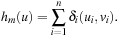 Another way for defining the FSM heuristic is by constructing the Boolean predicate f as
  . Applying the formula-based heuristic yields
  .
.
Since the distances between local states can be precomputed, each one can be gathered in constant time resulting in an overall time complexity that is linear to the number of processes of the system.
In contrast to the Hamming distance, the FSM distance abstracts from the current queue load and from values of the local and global variables. We expect that the search will then be directed into equivalent error states that could potentially be reachable through shortest paths. The reason is that some kind of errors depend on the local state of each component process, while variables play no role.
16.2.4. Liveness Model Checking
The liveness as safety model checking approach proposes to convert a liveness model checking problem into a safety model checking problem by roughly doubling the state vector size. The most important observation is that the exploration algorithms do not have to be rewritten.
In the lifted search space we search for shortest lasso-shaped counterexamples, without knowing the start of the cycle beforehand. We use the consistent heuristic of distances in N for finding accepting states in the original search space.
States in the lifted search space are abbreviated by tuples  , with u recording the start state of the cycle, and v being the current search state. If we reach an accepting state, we immediately switch to a secondary search. Therefore, we observe two distinct cases: primary search, for which the accepting state has not yet reached; and cycle detection search, for which an accepting state has to be revisited. The state
  reached in secondary search is the goal. Because it is a successor of a secondary state, we can distinguish the situation from reaching such a state for the first time.
For all extended states  in the lifted search space, let
  and
and  . Now we are ready to merge the heuristics to one estimate:
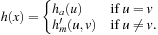 As each counterexample has to contain at least one accepting state in N, for primary states x we have that
  is a lower bound. For secondary states x, we have
 a lower bound to close the cycle and the lasso in total. Therefore, h is admissible. Moreover, we can strengthen the result.
(16.1)
It is not difficult to see that h is consistent; that is,  for all successor states
  of x. As both
  and
and  are monotone, only one of them is true at a time. Hence, we have to show that h is monotone in case of reaching an accepting state. Here we have that a predecessor x with an evaluation of
  spawns successors
  with evaluation values of
  . However, this incurs no problem as
  preserves monotonicity.
The model checking algorithm for directed external LTL search is an extension of external A* (see Ch. 8), which traverses the bucket file list along growing  diagonals. On disk we store (packed) state pairs. Figure 16.7 illustrates a prototypical execution.
16.2.5. Planning Heuristics
To encode communication protocols in PDDL, each process is represented by a finite-state automaton. Since is not difficult to come up with a specialized description, we are interested in a generic translation routine; the propositional encoding should reflect the graph structures of the processes and the communication queues.
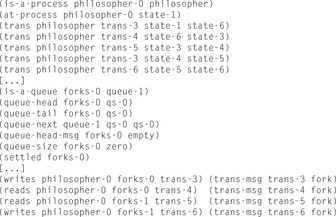
In the example problem for converting the Dining Philosophers problem (see Ch. 10) the initial state is shown in Figure 16.8.
 |
| Figure 16.8 |
The encoding of the communication structure is based on representing updates in the channel as changes in an associated graph. The message-passing communication model realizes the ring-based implementation of the queue data structure. A queue is either empty (or full) if both pointers refer to the same queue state. A queue may consist of only one queue state, so the successor bucket of queue state 0 is the queue state 0 itself. In this case the grounded propositional encoding includes actions where the add and the delete lists share an atom. Here we make the standard assumption that deletion is done first. In Figure 16.8 (bottom) the propositions for one queue and the connection of two queues to one process are shown.
Globally shared and local variables are modeled using numerical variables. The only difference of local variables compared to shared ones is their restricted visibility scope, so that local variables are simply prefixed with the process in which they appear. If the protocol relies on pure message passing, no numerical state variable is needed, yielding a pure propositional model for the Dining Philosophers problem.
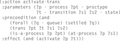
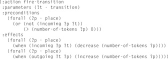
The PDDL domain encoding uses seven actions, named activate-trans, queue-read, queue-write,advance-queue-head, advance-empty-queue-tail, advance-nonempty-queue-tail, and process-trans. We show the activation of a process in Figure 16.9.
 |
| Figure 16.9 |
Briefly, the actions encode the protocol semantics as follows. Action activate-trans activates a transition in a process of a given type from local state  to
to  . Moreover, the action sets the predicate activate. This Boolean flag is a precondition of the queue-read and queue-write actions, which set propositions that initialize the reading/writing of a message. For queue Q in an activated transition querying message m, this corresponds to the expression Q?m, respectively Q!m. After the read/write operation has been initialized, the queue update actions:advance-queue-head, advance-empty-queue-tail, or advance-nonempty-queue-tail have to be applied. The actions respectively update the head and the tail positions, as needed to implement the requested read/write operation. The actions also set a settled flag, which is a precondition of every queue access action. Action process-trans can then be invoked. It executes the transition from local state
  to
to  ; that is, sets the new local process state and resets the flags.
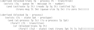
If the read message does not match the requested message, or the queue capacity is either too small or too large, then the active local state transition will block. If all active transitions in a process block, the process itself will block. If all processes are blocked, we have a deadlock in the system. Detection of such deadlocks can be implemented, either as a collection of specifically engineered actions or, more elegantly, as a set of derived predicates. In both cases we can infer, along the lines of argumentation outlined earlier, that a process/the entire system is blocked. The goal condition that makes the planners detect the deadlocks in the protocols is simply a conjunction of atoms requiring that all processes are blocked. The PDDL description for the derivation of a deadlock based on blocked read accesses is shown in Figure 16.10.
 |
| Figure 16.10 |
Extensions to feature LTL properties with PDDL are available via state trajectory constraints or temporally extended goals.
16.3. Program Model Checking
An important application of automated verification lies in the inspection of real software, because they can help to detect subtle bugs in safety-critical programs. Earlier approaches to program model checking rely on abstract models that were either constructed manually or generated from the source code of the investigated program. As a drawback, the program model may abstract from existing errors, or report errors that are not present in the actual program. The new generation of program model checkers builds on architectures capable of interpreting compiled code to avoid the construction of abstract models. The used architectures include virtual machines and debuggers.
We exemplify our considerations in program model checking on the object code level. Based on a virtual processor, it performs a search on machine code, compiled, for example, from a c/c++ source. The compiled code is stored in ELF, a common object file format for binaries. Moreover, the virtual machine was extended with multithreading, which makes it also possible to model-check concurrent programs. Such an approach provides new possibilities for model checking software. In the design phase we can check whether the specification satisfies the required properties or not. Rather than using a model written in the input language of a model checker, the developers provide a test implementation written in the same programming language as the end product.
In assembly language level program model checking there are no syntactic or semantic restrictions to the programs that can be checked as long as they can be compiled. Figure 16.11 displays the components of a state, which is essentially composed of the stack contents and machine registers of the running threads, as well as the lock- and memory-pools. The pools store the set of locked resources and the set of dynamically allocated memory regions. The other sections contain the program's global variables.
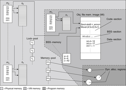
The state vector in Figure 16.11 can be large and we may conclude that model checking machine code is infeasible due to the memory required to store the visited states. In practice, however, most states of a program differ only slightly from their immediate predecessors. If memory is only allocated for changed components, by using pointers to unchanged components in the predecessor state, it is possible to explore large parts of the program's state space before running out of memory.
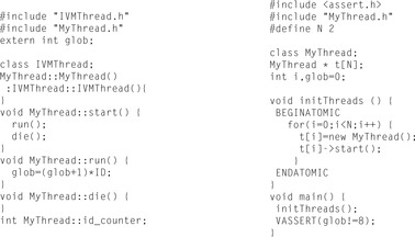
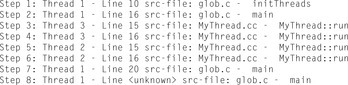
Figure 16.12 shows an example program, which generates two threads from an abstract thread class that accesses the shared variable glob. If the model checker finds an error trail of program instructions that leads to the line of the VASSERT statement, and the corresponding system state violates the Boolean expression, the model checker prints the trail and terminates. Figure 16.13 shows the error trail. The assertion is only violated if Thread 3 is executed before Thread 2. Otherwise, glob would take the values 0, 2, and 9.
Heuristics have been successfully used to improve error detection in concurrent programs. States are evaluated by an estimator function, measuring the distance to an error state, so that states closer to the faulty behavior have a higher priority and are considered earlier in the exploration process. If the system contains no error, there is no gain.
Deadlock Heuristics
The model checker automatically detects deadlocks during the program exploration. A thread can gain and release exclusive access to a resource using the statements VLOCK and VUNLOCK, which take as their parameter a pointer to a base type or structure. When a thread attempts to lock an already locked resource, it must wait until the lock is released by the thread that holds it. A deadlock describes a state, where all running threads wait for a lock to be released. An appropriate example for the detection of deadlocks is the most-block heuristic. It favors states, for which more threads are blocked.
Structural Heuristics
Another established estimate used for error detection in concurrent programs is the interleaving heuristic. It relies on a quantity for maximizing the interleaving of thread executions. The heuristic does not assign values to states but to paths. The objective is that by prioritizing interleavings concurrency bugs are found earlier in the exploration process.
The lock heuristic additionally prefers states with more variable locks and more threads alive. Locks are the obvious precondition for threads to become blocked and only threads that are still alive can get in a blocked mode in the future.
If threads have the same program code and the threads differ only in their (thread) ID, their internal behavior is only slightly different. In the thread-ID heuristic the threads are ordered linear according to their ID. This means that we avoid all those executions in the state exploration, where for each pair of threads, a thread with a higher ID has executed less instruction than threads with a lower ID. States that do not satisfy this condition will be explored later in a way not to disable complete exploration.
Finally, we may consider the access to shared variables. In the shared variable heuristic we prefer a change of the active thread after a global read or write access.
Trail-directed heuristics target trail-directed search; that is, given an error trail for the instance, find a possibly shorter one. This turns out to be an apparent need of the application programmer, for whom long error trails are an additional burden to simulate the system and to understand the nature of the faulty behavior.
Examples for the trail-directed heuristic are the aforementioned Hamming distance and FSM heuristics. In assembly language level program model checking the FSM heuristic is based on the finite-state automaton representation of the object code that is statically available for each compiled class.
The export of parsed programs into planner input for applying a tool-specific heuristic extends to include real numbers, threading, range statements, subroutine calls, atomic regions, deadlocks, as well as assertion violation detection. Such an approach, however, is limited by the static structure of PDDL, which hardly covers dynamic needs as present in memory pools, for example.
16.4. Analyzing Petri Nets
Petri nets are fundamental to the analysis of distributed systems, especially infinite-state systems. Finding a particular marking corresponding to a property violation in Petri nets can be reduced to exploring a state space induced by the set of reachable markings. Typical exploration approaches are undirected and do not take into account any knowledge about the structure of the Petri net.
More formally, a standard Petri net is a 4-tuple  , where
  is the set of places,
  is the set of transitions with
  , and
, and  . The backward and forward incidence mappings
  and
and  , respectively, map elements of
  and
and  to the set of natural numbers and fix the Petri net structure and the transition labels.
A marking maps each place to a number; with  we denote the number of tokens at place p. It is natural to represent M as a vector of integers.
Markings correspond to states in a state space. Petri nets are often supplied with an initial marking  , the initial state. A transition t is enabled if all its input places contain at least one token,
  for all
  . If a transition is fired, it deletes one token from each of its input places and generates one on each of its output places. A transition t enabled at marking m may fire and generate a new marking
  for all
  , written as
  .
.
A marking  is reachable from M, if
  , where
  is the reflexive and transitive closure of →. The reachability set
  of a Petri net N is the set of all markings M reachable from
  .
.
A Petri net N is bounded if for all places p there exists a natural number k, such that for all M in  we have
  . A transition t is live, if for all M in
  , there is a
  in
in  with
with  and t is enabled in
  . A Petri net N is live if all transitions t are live. A firing sequence
  starting at
  is a finite sequence of transitions such that
  is enabled in
  and
and  is the result of firing
  in
in  .
.
In the analysis of complex systems, places model conditions or objects such as program variables, transitions model activities that change the values of conditions and objects, and markings represent the specific values of the condition or object, such as the value of a program variable.
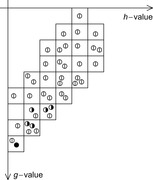
An example of an ordinary Petri net for the Dining Philosophers example with 2 and 4 philosophers is provided in Figure 16.14. Different philosophers correspond to different columns, and the places in the rows denote their states: thinking, waiting, and eating. The markings for the 2-philosophers case correspond to the initial state of the system; for the 4-philosophers case, we show the markings that resulted in a deadlock.
There are two different analysis techniques for Petri nets: the analysis of the reachability set and the invariant analysis. The latter approach concentrates on the Petri net structure. Unfortunately, invariant analysis is applicable only if studying  is tractable. Hence, we concentrate on the analysis of the reachability set. Recall that the number of tokens for a node in a Petri net is not bounded a priori, so that the number of possible states is infinite.
Heuristics estimate the number of transitions necessary to achieve a condition on the goal marking. Evaluation functions in the context of Petri nets associate a numerical value to each marking to prioritize the exploration of some successors with respect to some others. The shortest firing distance  in a net N is defined as the length of the shortest firing sequence between M and
  . The distance is infinite if there exists no firing sequence between M and
  . Moreover,
  is the shortest path to a marking that satisfies condition
  starting at M,
  . Subsequently, heuristic
  estimates
  . It is admissible, if
  and monotone if
  for a successor marking
  of M. Monotone heuristics with
  for all
  are admissible.
We distinguish two search stages. In the explanatory mode, we explore the set of reachable markings having just the knowledge on what kind of error  we aim at. In this phase we are just interested in finding such errors fast, without aiming at concise counterexample firing sequences. For the fault-finding mode we assume that we know the marking where the error occurs. This knowledge is to be inferred by simulation, test, or a previous run in the explanatory mode. To reduce the firing sequence a heuristic estimate between two markings is needed.
Hamming Distance Heuristic
A very intuitive heuristic estimate is the Hamming distance heuristic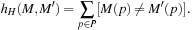 Here, the truth of
  is interpreted as an integer in
  . Since a transition may add or delete more than one token at a time, the heuristic is neither admissible nor consistent. However, if we divide
  by the maximum number of infected places of a transition, we arrive at an admissible value. In the 4-Dining Philosophers problem, an initial estimate of 4 matches the shortest firing distance to a deadlock.
Subnet Distance Heuristic
A more elaborate heuristic that approximates the distance between M and  works as follows. Via abstraction function
  it projects the place transition network N to
  by omitting some places, transitions, and corresponding arcs. In addition, the initial set of marking M and
  is reduced to
  and
and  . As an example, the 2-Dining Philosophers Petri net in Figure 16.14 (left) is in fact an abstraction of the 4-Dining Philosophers Petri net to its right.
The subnet distance heuristic is the shortest path distance required to reach  from
from  , formally
 In the example of 4-Dining Philosophers we obtain an initial estimate of 2. The heuristic estimate is admissible, i.e.,
  . Let M be the current marking and
  be its immediate successor. To prove that the heuristic
  is consistent, we show that
 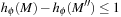 . Using the definition of
  , we have that
 This inequality is always true since the shortest path cost from
  to
to  cannot be greater than the shortest path cost that traverses
  (triangular property).
To avoid recomputations, it is appropriate to precompute the distance prior to the search and to use table lookups to guide the exploration. The subnet distance heuristic completely explores the coverage of  and runs an All Pairs Shortest Paths algorithm on top of it.
If we apply two different abstractions  and
and  , to preserve admissibility, we can only take their maximum,
 However, if the supports of
  and
and  are disjoint—that is, the corresponding set of places and the set of transitions are disjoint
  and
and  —the sum of the two individual heuristics
 is still admissible. If we use an abstraction for the first two and the second two philosophers we obtain the perfect estimate of four firing transitions.
Activeness Heuristic
While the preceding two heuristics measure the distance from one marking to another, it is not difficult to extend them for a goal by taking the minimum of the distance of the current state to all possible markings that satisfy the desired goal. However, as we concentrate on deadlocks, specialized heuristics can be established that bypass the enumeration of the goal set.
A deadlock in a Petri net occurs if no transition can fire. Therefore, a simple distance estimate to the deadlock is simply to count the number of active transitions. In other words, we have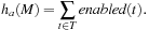 As with the Hamming distance the heuristic is not consistent nor admissible, since one firing transition can change the enableness of more than one transition. For our running example we find four active transitions in the initial states.
Planning Heuristics
In the following we derive a PDDL encoding for Petri nets, so that we can use in-built planning heuristic to accelerate the search. We declare two object types place and transition. To describe the topology of the net we work with the predicates (incoming ?s - place ?t - transition) and (outgoing ?s - place ?t - transition), representing the two sets  and
and  . For the sake of simplicity all transitions have weight 1. The only numerical information that is needed is the number of tokens at a place. This marking mapping is realized via the fluent predicate (number-of-tokens ?p - place). The transition firing action is shown in Figure 16.15.
The initial state encodes the net topology and the initial markings. It specifies instances to the predicates incoming and outgoing and a numerical predicate (number-of-tokens) to specify  . The condition that a transition is blocked can be modeled with a derived predicate as follows:
(:derived blocked (?t - transition)
(exists (?p - place)
(and (incoming ?p ?t) (= (number-of-tokens ?p) 0))))
Consequently, a deadlock to be specified as the goal condition is derived as
(:derived deadlock (forall (?t - transition) (blocked ?t)))
It is obvious that the PDDL encoding inherits a one-to-one correspondence to the original Petri net.
16.5. Exploring Real-Time Systems
Real-time model checking with timed automata is an important verification scenario, and cost-optimal reachability analysis as considered here has a number of industrial applications including resource-optimal scheduling.
16.5.1. Timed Automata
Timed automata can be viewed as an extension of classic finite automata with clocks and constraints defined on these clocks. These constraints, when corresponding to states, are called invariants, and restrict the time allowed to stay at the state. When connected to transitions these constraints are called guards. They restrict the use of the transitions. The clocks C are real-valued variables and measure durations. The values of all the clocks in the system are denoted as a vector, also called clock valuation function,  . The constraints are defined over clocks and can be generated by the following grammar: For
  , a constraint
  is defined as
 where
where  and
and  . These constraints yield two different kinds of transitions. The first one (delay transition) is to wait for some duration in the current state s, provided the invariant
  holds. This lets only the clock variables increase. The other operation (edge transition) resets some clock variables while taking the transition t. The operation is possible given that the guard
  holds. We allow an edge transition to be taken without an increase in time.
Trajectories are alternating sequences of states and transitions and define a path within the automata. The reachability task is to determine if the goal in the form of partial assignment to the ordinary and clock variables can be reached or not. The optimal reachability problem is to find a trajectory that minimizes the overall path length.
For a reachability analysis on timed automata, we face the problem of an infinite-state space. This infiniteness is due to the fact that the clocks are real-valued and, hence, an exhaustive state space exploration suffers from infinite branching. This problem was solved with the introduction of a partitioning scheme based on regions. A region automata creates finitely many partitions of the infinite-state space based on the equivalent classes of the clock valuations. In model checking tools, though, a coarser representation called a zone is used. Formally, a zone Z over a set of clocks C is a finite conjunction of difference constraints of the form  or
or  , with
  and integer d. 1
The semantics for delay and edge transitions in a timed automata are based on some basic operations. We restrict to changes in clock variables. For a clock vector u and a zone Z we write  if u satisfies the constraints in Z. The two main operations on (clock) zones are: clock reset
  that resets all the clocks x, and delay (d time units)
  . The reachability problem in timed automata can then be reduced to the reachability analysis in zone automata. In a zone automata, each state is basically a symbolic state corresponding to one or many states in the original timed automata. The new state is represented as a tuple
  , with l being the discrete part containing the local state of the automata, and Z is the convex
  -dimensional hypersurface in Euclidean space. Semantically,
  now represents the set of all states
  with
with  . Let
. Let  denote the set of constraints defined on clocks C and let
  denote the power set of C. Formally, a timed automata is a tuple
  , where S is the set of states,
  is the initial state with an empty zone,
  is the transition relation making states to their successors, given the constraints on the edge are satisfied,
  assigns invariants to the states, and T is the set of final states.
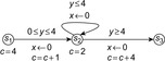
16.5.2. Linearly Priced Timed Automata
Linearly priced timed automata are timed automata with (linear) cost variables. For the sake of brevity, we restrict their introduction to one cost variable c. Cost increases at states with respect to a predefined rate and in transitions with respect to an update operation. The cost-optimal reachability problem is to find a trajectory that minimizes the overall path costs. Figure 16.16 shows a timed automata. The minimum cost of reaching location  with cost 13 corresponds to the trajectory
  of waiting 0 steps in
  and then taking the transition to
  , where four time steps are spent until the transition to the goal in
  .
.
 |
| Figure 16.16 |
Similar to timed automata, for priced timed automata we use the notion of priced zones to represent the symbolic states. Let  be the unique clock valuation of Z such that for all
  and
and  , we have
  ; that is, it represents the lowest corner of the
  -dimensional hyper-surface representing a zone. In the following,
  is referred to as the zone offset. For the internal state representation, we exploit the fact that prices are linear cost hyperplanes of zones. A priced zone
  is a triple
  , where Z is a zone, integer c describes the cost of
  , and
, and  gives the rate for a given clock. In other words, prices of zones are defined by the respective slopes that the cost function hyperplane has in the direction of the clock variable axes. Furthermore, with
  , we denote the cost evaluation function based on priced zones
  . The cost value f for a given clock
  in the priced zone
  can then be computed as
  . Formally, a linearly priced timed automata over clocks C is a tuple
  , where S is a finite set of locations;
  is the initial state with empty priced zone
  ;
;  is the set of transitions, each consisting of a parent state, the guard on the transition, the clocks to reset, and the successor state;
  assigns invariants to locations; and
  assigns prices to the states and transitions.
16.5.3. Traversal Politics
In priced real-time systems, the costs f denote a monotonic increasing function implying that for all  we have
  . It is clear that breadth-first search does not guarantee a cost-optimal solution. A natural extension is to continue the search when a goal is encountered and keep on searching until a better goal is found or the state space is exhausted. Such a branch-and-bound algorithm is an extension to uninformed search and prunes all the states that do not improve on the last solution cost. Given that the cost function is monotone, the algorithm always terminates with an optimal solution. The underlying traversal policy for branch-and-bound can be borrowed from either breadth-first search, depth-first search, or best-first search.
Heuristics are either provided by the user, or inferred automatically by generalizing the FSM distance heuristic to include clock variables. The automated construction of the heuristic shares similarities with the ones for metric planning and is involved.
One of the involved differences between real-time reachability and ordinary reachability analysis is the zone inclusion check. In (delayed) duplicate elimination we omit all identical states from further consideration, whereas in real-time model checking we have to check inclusions of the form  to detect duplicate states. Once Z is closed under entailment, in the sense that no constraint of Z can be strengthened without reducing the solution set, the time complexity for inclusion checking is linear to the number of constraints in Z.
Subsequently, while porting real-time model checking algorithms to an external device, we have to provide an option for the elimination of zones. Since we cannot define a total order on zones, trivial external sorting schemes are useless in our case. In external breadth-first search we exploit the fact that two states  and
and  are comparable only when
  . This motivates the definition of zone union U, where all zones correspond to the states sharing a common discrete part l, and for all
  , we have
  . Duplicate states can now be removed by first sorting with respect to the discrete part l, which will cluster all states, sharing the same l-value, and then performing a one-to-one comparison among all such states. The result of this phase is a file where states are sorted according to the discrete parts l forming duplicate free zone unions. This one-to-one comparison of all the zones for a particular l can only be performed I/O-efficiently when all the states sharing the same l can be read into the main memory. The same approach of internalizing zone unions is available during set refinement with respect to predecessor files. We load both the zone union from the predecessor file and the one in the unrefined file and check for the entailment condition.
16.6. Analyzing Graph Transition Systems
Graphs are a suitable formalism for software and hardware systems involving issues such as communication, object orientation, concurrency, distribution, and mobility. The properties of such systems mainly regard aspects such as temporal behavior and structural properties. They can be expressed, for instance, by logics used as a basis for a formal verification method, the main success of which is due to the ability to find and report errors.
Graph transition systems extend traditional transition systems by relating states with graphs and transitions with partial graph morphisms. Intuitively, a partial graph morphism associated to a transition represents the relation between the graphs associated to the source and the target state of the transition; that is, it models the merging, insertion, addition, and renaming of graph items (nodes or edges), where the cost of merged edges is the least one among the edges involved in the merging.
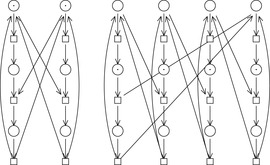
As an example, consider the Arrow Distributed Directory Protocol, a solution to ensure exclusive access to mobile objects in a distributed system. The distributed system is given as an undirected graph G, where vertices and edges, respectively, represent nodes and communication links. Costs are associated with the links in the usual way, and a mechanism for optimal routing is assumed.
The protocol works with a minimal spanning tree of G. Each node has an arrow that, roughly speaking, indicates the direction in which the object lies. If a node owns the object or is requesting it, the arrow points to itself; we say that the node is terminal. The directed graph induced by the arrows is called L. Roughly speaking, the protocol works by propagating requests and updating arrows such that at any moment the paths induced by arrows, called arrow paths, either lead to a terminal owning the object or waiting for it.
More precisely, the protocol works as follows: Initially, L is set such that every path leads to the node owning the object. When a node u wants to acquire the object, it sends a request message  to
to  , the target of the arrow starting at u, and sets
  to u; that is, it becomes a terminal node. When a node u of which the arrow does not point to itself receives a
  message from a node v, it forwards the message to node
  and sets
  to v. On the other hand, if
  (the object is not necessarily at u but will be received if not) the arrows are updated as in the previous case, but this time the request is not forwarded but enqueued. If a node owns the object and its queue of requests is not empty, it sends the object to the (unique) node u of its queue sending a
  message to v. This message goes optimally through G. Figure 16.17 illustrates two states of a protocol instance with six nodes
  .
.
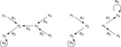
We might be interested in properties like Can node  be a terminal? Can node
  be terminal and all arrow paths end at
  ? Can a node v be terminal? Can a node v be terminal and all arrow paths end at v ?
The properties of a graph transition system can be expressed using different formalisms. We can use, for instance, a temporal graph logic, which combines temporal and graph logics. A similar alternative is spatial logics, which combines temporal and structural aspects. In graph transformation systems, we can use rules to find certain graphs: The goal might be to find a match for a certain transformation rule. For the sake of simplicity and generality, however, we consider that the problem of satisfying or falsifying a property is reduced to the problem of finding a set of goal states characterized by a goal graph and the existence of an injective morphism.
It is of practical interest to identify particular cases of goal functions as the following goal types: (1)  is an identity—the exact graph G is looked for; (2)
  is a restricted identity—an exact subgraph of G is looked for; (3)
  is an isomorphism—a graph isomorphic to G is looked for; (4)
  is any injective graph morphism—the most general case.
Note that there is a type hierarchy, since goal type 1 is a subtype of goal types 2 and 3, which are of course subtypes of the most general goal type 4. The computational complexity of the goal function varies according to the previous cases. For goals of types 1 and 2, the computational efforts needed are just  and
and  , respectively. Unfortunately, for goal types 3 and 4, due to the search for isomorphisms, the complexities increase to a term exponential in
  for Graph Isomorphism and to a term exponential in
  for Subgraph Isomorphism.
We consider two analysis problems. The first one consists of finding a goal state, and the second problem aims at finding an optimal path to a goal state. The two problems can be solved with traditional graph exploration algorithms. For the reachability problem, for instance, we can use depth-first search, hill-climbing, best-first search, Dijkstra's algorithm (and its simplest version, breadth-first search), or A*. For the optimality problem, only the last two are suitable.
Removable Items Heuristic
For graph transformation systems, graph morphisms are induced by graph transformation rules while in communication protocols by the operations of the processes. In most cases, such transitions are usually local and involve a few insertions/deletions/mergings of items. As a heuristic we can thus determine, prior to the analysis, the number of items deleted and erased by graph morphisms so that it is not difficult to derive consistent heuristics.
Isomorphism Heuristics
The main drawback of the preceding for goals of type 4 is evident. If state graphs have more edges and nodes than the goal graph the resulting heuristic is completely blind. Thus, we propose functions inspired by heuristics to decide Graph Isomorphism or Subgraph Isomorphism. For instance, if we have to decide whether two graphs are isomorphic, we would check first whether the two graphs have the same number of items. If so, we could continue trying to match nodes with the same in- and out-degrees.
Obviously, none of the two heuristics presented in this section is consistent or admissible in general, and we could define other versions of the heuristics by changing some of the parameters used: the order criteria, the distance between vectors, and so on. The idea of these heuristics is, indeed, to illustrate the wide variety of nonadmissible heuristics we could define.
Hamming Distance Heuristic
The Hamming distance of two bit vectors is the number of vector indices on which the bits differ. As there are many different encodings of a graph, we choose a simple one based on the image of the state representation in the memory. As more than one bit can change within one transition (e.g., the last one before reaching the goal), the heuristic is neither admissible nor consistent.
Planning Heuristics
Finally, we can profit from specific heuristics available in the concrete tool that performs the analysis. To apply a planner to graph transition systems, we first need a propositional description of graph transition systems in PDDL. Due to the parametric description facility provided by planning formalism, it is easy to define morphisms and partial morphisms as actions. For example, a morphism that inverses an edge can be specified as follows:
(:action morphism-inverse
:parameters(?u ?v - node)
:precondition (and (link ?u ?v))
:effect
(and (not (link ?u ?v)) (link ?v ?u)))
A graph transition problem can be described with the help of predicates defining the graph in the initial state. The whole graph can be described by the use oflinkpredicates defining the edges between different nodes of the graph.
Fortunately, PDDL provides a very neat and elegant mechanism to formulate our goals' criteria. In the following we address methods to describe the following goals.
Property 1 goal (subgraph): Perhaps the most simple to describe are the type 1 goals, as we only search for a specific subgraph. As is evident from the PDDL specification of the domain, the subgraph can easily be declared by using the (link u v) predicates.
Property 2 goal (exact graph): For a Property 2 goal, we look for an exact matching of the goal graph in the state space. Just like for the previous type, we can describe the whole graph with (link u v) predicates.
Property 3 goal (subgraph isomorphism): Given a goal graph G, the state space is searched for a state that contains a subgraph isomorphic to G. In such cases, goals are strictly more expressive and need an existential quantification over all the nodes to be described succinctly. A goal of type 3 can then be included as
(:goal (exists (?n0 ?n1 - node) (link ?n0 ?n1))
Property 4 goal (isomorphism): Given a goal graph G, the state space is searched for a node that contains a graph isomorphic to G. Having the existential quantifier in our hands, we can describe G using(link u v)predicates, for example,
(:goal (exists ?n0 ?n1 ?n2 ?n3 ?n4 ?n5 - node)
(and (link ?n0 ?n0) (link ?n1 ?n0) (link ?n2 ?n0) (link ?n3 ?n1)
(link ?n4 ?n0) (link ?n5 ?n4))
In practice, heuristic search planners can outperform general tools for verifying graph transition systems. But, similar to program model checking applications, the static structure of a plan that models the approach is not able to cover dynamic behaviors in graph transition systems.
16.7. Anomalies in Knowledge Bases
Knowledge-based systems (KBSs) are used in several applications. Especially when applied to business settings, errors in a KBS can cause considerable damage. Most KBSs are rule based. Checking for anomalies in a given knowledge-based system is a very important task. A popular classification of such anomalies are
1. Redundancy: A rule can be omitted without affecting the system's inferences.
2. Conflict: Incompatible inferences can be made from valid initial data.
3. Circularity: An inference depends on itself.
4. Deficiency: No useful conclusions are produced for some valid input set.
Consider the following example for determining the academic status of a person with a knowledge base consisting of five rules:
• (R1): 
• (R2): 
• (R3): 
• (R4): 
• (R5): 
Moreover, let  ,
,  , and
, and  be the possible inputs and
  ,
,  , and
, and  be mutually incompatible outputs. To check this rule base, goals are labeled. As the first goal is reachable via two paths (via rule R4 or via rules R1 and R2), we get two possible environments:
  and
and  , so that we obtain a redundancy. The rule base also contains a conflict, namely the conjunction of
  , and
, and  contains the valid combination
  .
.
The efficiency of a labeling approach clearly depends on the compactness of the generated labels. It is not difficult to see that these may require exponential size, with the exponent being in the depth of the rule sets. Henceforth, more efficient representations like BDDs are needed.
The symbolic approach encodes the system's input in binary form, traverses the rule base, thereby constructing the BDDs instead of labels that describe the input and output dependencies of the system, checking these BDD labels against each other, and reporting any anomaly.
In the example we can choose a three-bit unary encoding  , respectively denoting the truth or absence of the inputs
  ,
,  , and
, and  . Traversing the rule base either by forward or backward chaining gives the BDD representation for the labels. For every rule instance in the inference space, a BDD is constructed using the labels of the literals in its antecedent. The label of the corresponding hypothesis is obtained by computing the disjunct of the rule labels of all rule instances having that hypothesis as a consequent. In the example we obtain the BDD representations for undergraduate
  , for graduate
  , and for staff
  . The redundancy anomaly is found during exploration by performing a containment operation on the set of BDD labels. The incompatible output anomaly is established by conjoining the output BDDs for undergraduate
  and for staff
  .
.
16.8. Diagnosis
In diagnosis, we are not only concerned with detecting errors, but additionally with explaining them. Application areas for such (model-based) diagnosis are intelligent tutoring, intelligent authoring, and intelligent debugging systems, in which the mistakes of a novice student, author, or programmer have to be uncovered based on a model of an experienced one. The scenario differs from detecting errors in formal verification as introduced for directed model checking as one practical application of heuristic search technology.
Finding a good diagnosis with respect to some existing flaws in a system is a guided search in itself. Once we have found a misconception, we have to search for the flaw in the argumentation according to the subject model of the problem. This is done by propagating the error in the model and probing on more and more specific issues. The subject model or qualitative dependency network is an augmented undirected graph that is generated in a process called qualitative simulation. The edges represent discrete variables with values of a certain range. In the easiest case a variable is Boolean stating that a condition is true or false (the velocity of a car is positive). In other cases a variable represents a set of quantities (the acceleration of a car is large). The nodes in the network manipulate and propagate the information found at incident edges. They represent the qualitative knowledge and the influence the variables have on each other (if the velocity of a car is positive and the brakes are pushed, the velocity will decrease).
Dependency networks are constructed by an expert, explored in an empirical study, or inferred with an inductive learning algorithm. In the diagnosis task we match the knowledge of the learner to the network. The main objective is to efficiently store and propagate the input information within the network. If a misconception arises, we aim to pose only a few questions to pinpoint a wrong inference. In our scenario we allow the learner to make multiple faults according to the model and simulate all possible worlds he or she might be in. Since a diagnosis task is a search in a space of different hypothesis on the values of variables, we deal with uncertainties in background knowledge.
16.8.1. General Diagnostic Engine
The general diagnostic engine (GDE) is a framework for performing model-based diagnostics. It is traditionally exemplified by arithmetic dependency networks, in which we have devices such as adders ( ) and multipliers (
 ). Edges connect the devices as illustrated in Figure 16.18 to an overall graph structure. Variables labeling the edges can be assigned to specific values and the information according to the setting is broadcast within the network. Devices can malfunction and therefore lead to contradictions. The set of possible assignments to the variables is restricted to a small integer range. This implies that all different values can be encoded using only a few bits. A probe of an edge is an assignment to a variable that reflects the supervised background knowledge received in an interaction with the learner. The access to this knowledge is often computationally expensive.
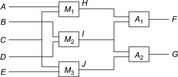
We distinguish two main stages in one iteration of a GDE. On one hand, we have to update the model according to a given probe, and on the other hand, we have to discriminate the candidates for the next probe. In the following we focus on the first issue. GDE is based on an architecture called assumption-based truth maintenance system (ATMS). Besides the dependency network structure, an ATMS maintains database entries  , with v being an assignment to a variable and
  being its justification. A justification is a set of devices that have been used to derive that variable V is assigned to v. Different justifications for a single variable value might exist. Starting with an empty database the learner instantiates variables one after the other. These variables are final, since we have full knowledge of their values. The consequences are drawn with respect to the functionality of the used devices and lead to an assumption on the valuation of the other variables in the network. If the assumption is not confirmed by the learner, we call a value a no-good.
In the example the assignments A to 1, B to 1, C to 1, and D to 1 forces F to equal 2 with justification  . The assignment F to 1 is a no-good. Unfortunately, the approach to propagate the values in the network with a simple depth-first search is not sufficient. We need some form of iteration. The new information has to be propagated in the network until no further changes can be achieved, and it has to be offered at every edge of each device node. The database at device node k with degree n for the operation
  is updated as follows: Take every combination of entries
  for the variables
  , calculate
  with justification
  , and insert the pair
  into the database. Especially in large models these efforts are tremendous, such that merging the inputs reveals the bottleneck of the overall propagation.
16.8.2. Symbolic Propagation
The set of possible propagations of variables in a discrete domain at a given device consists of instantiations to the incident variables  . As seen earlier, BDDs can be utilized to efficiently describe sets of states. In the case of a diagnosis problem a state is a pair consisting of a variable assignment and set of devices that causes the variable to have this particular value.
We have already seen that if we restrict the values to a finite domain, we can represent the Boolean operations Add and Mult with parameters a, b, and c in the form of a BDD. The key idea in using BDDs is that they do not only apply to a single element but to the whole set that is described at the inputs. For example, combining the BDD characterization of the set  with the BDD representation of
  and with the BDD for Mult directly leads to the description of the BDD representation for the set
  . Moreover, the relational description allows us to apply the BDDs in the reverse direction. For example, the Subtract and Div operators can be obtained by swapping the variable sets a and c in Add and Mult.
Let  and
and  be the BDD representations of the different value assignments of the input variables for a device that realizes a Boolean function
  . The relational product
  computes the desired output BDD. The other two propagation rules are obtained similarly. The justification of the result can be derived by merging the justifications of the inputs. We extend the result with the influence of the currently operating unit and we only allow to execute the operation if both inputs do not already rely on the unit. Therefore, we build the BDD Result based on the disjunct on all triples of justifications satisfying these additional constraints. As the number of units n and thus the number of bits to encode a justification are big and the power set is exponential in n, we might doubt that this BDD can be constructed, but we explicitly build the BDD for
  on every index i and build the conjunct for all
  .
.
Let  be the description of the first input and
  be the description of the second input. Then we have
The implementation of the proposed diagnosis system based on BDDs is simple. Any diagnostic variable consists of a marker final, a BDD bdd representing all possible value/justification pairs, and the variable sets for addressing value and just. Diagnostic variables are linked to at least two devices to inform the devices if a change to a BDD has been obtained. There are four cases to terminate the propagation:
• The output is final: We have full knowledge of the output values.
• One input BDD is the zero function: We prevent propagation.
• The output BDD is the zero function: Either the computation on the restricted domain is not possible or one boundary condition to the relation Result is met.
• The result implies the output BDD: The output value has already been calculated or no new information is available.
16.9. Automated Theorem Proving
Standard theorem proving procedures draw inferences on sets of clauses. For theorem proving in predicate logic SAT solver technology is frequently applied.
To illustrate how automated theorem proving can be casted a variant to state space search we recall the resolution rule for predicate logic. From sentences  and
and 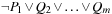 we derive resolvents
  , for example, from P and
  , we derive Q.
In first-order logic we are given sentences  and
and  , where each
  and
and  is a literal. If
  and
and  unify with substitution list
  , we can derive the resolvent sentence subst
  . For example, from clauses
  and
and 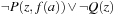 , we can derive the resolvent clause
 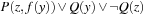 using
using  .
.
Unification itself is a pattern matching procedure, which takes two atomic sentences, called literals, as input, returns failure if no match is obtained, and a substitution list,  , if a match is found. The equation
  means
means  for two atomic sentences p and q, where
  is called the most general unifier (mgu), variables are implicitly universally quantified, and to make literals match, we replace variables by terms. Examples are
  ,
,  ,
,  ,
,  with mgu
  ,
,  ,
,  , and
, and 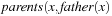 ,
,  ,
,  with unification failure.
The pseudo-code linear-time algorithm that returns the mgu is provided in Algorithm 16.1. Note that the mgu not unique, the variable can never be replaced by a term containing that variable, and it is important to check occurrences before making a recursive call.
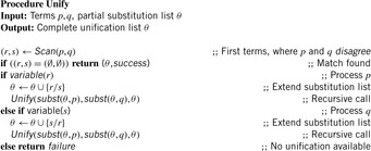

The resolution refutation procedure realizes proof-by-contradiction with an implementation displayed in Algorithm 16.2. Given a consistent set of axioms  and a goal sentence Q, we have to show that
  ; that is, every interpretation I that satisfies
  satisfies Q. Since interpretation I either satisfies Q or
  , we have
  if and only if
  .
.
Since the resolution rule is only applicable with sentences that are in the form  , the question remains, how to convert every sentence in first-order logic into this form. Fortunately, every sentence in first-order logic can be converted to a logically equivalent sentence that is in a normal form called clause form.
The nine steps to obtain a clause form are as follows. First, we eliminate all equivalences by replacing each instance of the form  with the equivalent expression
  . Then we eliminate all implications by replacing each instance of the form
  with
with  . Next, we reduce the scope of each negation symbol to a single predicate by applying equivalences such as converting
  to P;
to P;  to
to  ;
;  to
to  ;
;  to
to  ; and
; and  to
to  . Afterward, we standardize the variables and rename all variables so that each quantifier has its own unique variable name; convert
  to
to  if there is another place where variable x is already used. Next, we eliminate existential quantification by introducing Skolem functions; that is, convert
  to
to  , where c is a brand new constant symbol that is not used in any other sentence. Value c is called a Skolem constant. More generally, if the existential quantifier is within the scope of a universal quantified variable, then introduce a Skolem function that depends on the universally quantified variable. Function f is called a Skolem function, and must be a new name that does not occur in any other sentence in the entire KB. Subsequently, we remove universal quantification symbols by first moving them all to the left end and making the scope of each the entire sentence, and then just dropping the first part. Afterward, we distribute and over or to obtain a conjunction of disjunctions. Next, we split each conjunct into a separate clause. Finally, we standardize variables so that each clause contains unique variable names.
The resolution procedure can be thought of as the bottom-up construction of a search tree, where the leaves are the clauses produced by KB and the negation of the goal. When a pair of clauses generates a new resolvent clause, we add a new node to the tree with arcs directed from the resolvent to the two parent clauses. It succeeds when a node containing the false clause is produced, becoming the root node of the tree. This suggests a breadth-first exploration. Level 0 clauses are those from the original axioms and the negation of the goal. Level k clauses are the resolvents computed from two clauses, one of which must be from Level  and the other from any earlier level. Breadth-first exploration is complete, but very inefficient.
To control the resolution's search, different suggestions have been made. The set-of-support approach requires that at least one parent clause must be from the negation of the goal or one of the descendants of such a goal clause. The strategy is complete, when we assume that all possible set-of-support clauses are derived. In unit resolution, at least one parent clause must be a unit clause, one containing a single literal. This strategy is not complete in general, but complete for Horn clauses. For input resolution, at least one parent from the set of original clauses (from the axioms and the negation of the goal) strategy is not complete in general, but complete for Horn clauses.
16.9.1. Heuristics
A top-down proof creates a proof tree, where the node label of each interior node corresponds to the conclusion, and the node labels of its children correspond to the premises of an inference step. Leaves of the proof tree are either axioms or instances of settled theorems. A proof state represents the outer fragment of a proof tree: the top node represents the goal and all leaves representing the subgoals of the proof state. All proven leaves can be discharged, because they are not needed for further considerations. If all subgoals have been solved, the proof is successful.
One estimate for the remaining distance to the goal is the number of internal nodes of the current proof state. An illustrative competitor is the string length of a proof state representation. The number of trees with k internal nodes and the number of strings with length k are both finite, such that for this internal node heuristic and the string length heuristic the number of proof states with fixed heuristic value k are finite.
This is the basis for the design of guided search algorithms with guaranteed progress. At first glance, heuristic search according to the representation size of a theorem seems not to be a good choice, since it exploits very poor knowledge. But even these vague parts of information can speed up computation by magnitudes.
The third heuristic we suggest is the number of open subgoals in the current proof state. This heuristic is the only one that is admissible when we assume that one inference step can close at most one open subgoal at a time. This also proves that the open subgoal heuristic is consistent.
In contrast to the internal node heuristic and the string length heuristic by the limited range of information, the open subgoal heuristic can have infinite plateaus of states with the same estimate value. In this case, greedy best-first search frequently fails to terminate. On the other hand, in regular state spaces, even weaker heuristics may yield fast solutions in greedy search.
16.9.2. Functional A* Search
In a forward proof, axioms and already proven theorems are combined to generate new theorems. In a backward proof, we start with the theorem to prove, which is step-by-step reduced to new subgoals. With a tactic, basic inference steps are combined to larger case-sensitive and proof-searching rules using axioms, memorized theorems, or assumptions. For increasing performance in some basic object logics, tableau theorem provers have been integrated, but their inference is not generic for all object logics. The inference process is hidden in the auto tactic.
Greedy best-first search expands the states with minimal evaluation function value first. It is attracted by local optima not complete even for finite graphs. In contrast, DFS and BFS are complete since DFS uses global memory to store already proven subgoals, and BFS could omit the pruning of duplicate states.
In a functional implementation of A* (see Alg. 16.3), one input parameter is the heuristic function h(we have not expelled the input and output parameters since the input are all mappings and the function declaration itself is assigned to the output). Furthermore, the successor generation function  , goal predicate Goal, and the initial state s are passed to the algorithms as parameters, where the goal function helps filtering the successor states. The priority queue Open is represented by a list of triples
  , sorted by ascending f-values. For the sake of brevity we have omitted reopening of already expanded nodes on shorter generating paths. If the heuristic function h is consistent,
  for all
  , this is no restriction. In this case, on every path the priority f is monotone. All reweighted edges are positive, and the correctness argument of Dijkstra's algorithm applies. All extracted nodes will have correct f-values. The implementation of A* in Algorithm 16.3 uses simultaneous recursion. Keywords and function declarations are set in bold and variables and function calls are set in italics.
In contrast to the imperative setting, in functional A*, insert implements dictionary updates within the set of horizon nodes. If the state is already contained in the priority queue, no insertion takes place, thus avoiding duplicates within the queue. However, since the Closed list of already expanded states is not modeled, even on finite graphs the functional pure heuristic search derivate  is no longer complete.
Global expanded node maintenance in Closed is integrated in the pseudo codes of Algorithm 16.3 as follows: Set Closed is supplied as an additional parameter—in A* to the relax function, and in IDA* to the depth function. In A*, Closed is initialized to the empty list at the very beginning, while in IDA*, Closed is reinitialized in each iteration. Instead of (map f visited states are first eliminated by (map f
  . The dictionary for Closed can be implemented through lists, balanced trees, or low-level hash tables.

16.10. Bibliographic Notes
Approver by Hajek (1978) is probably the first tool for the automated verification of communication protocols. It has already applied guidances to search the state space. The tool was capable of dealing with a broader class of concurrent systems than the classic communication protocols, for instance, like mutual exclusion algorithms. The SpotLight system by Yang and Dill (1998) has applied A* to combat the state explosion problem. A general search strategy, called the target enlargement analysis, computed nodes around the goal by applying some preimages starting from the target description before starting the forward search. With this respect, this technique shares similarities with perimeter search (see Ch. 9). A first study of symbolic-guided model checking algorithm simulating the A* exploration has been provided by Reffel and Edelkamp (1999).
Heuristic search model checking for the analysis of communication protocols has been suggested by Edelkamp, Leue, and Lluch-Lafuente (2004b). The authors coined the term directed model checking and implemented a guided variant of the explicit-state model checker SPIN (Holzmann, 2004). For liveness properties the authors contribute an improved nested-DFS algorithm based on the classification of the automata representation of the property in strongly connected components. Later, trail-improvement and partial-order reduction has been included to the system (Edelkamp, Leue, and Lluch-Lafuente, 2004c). Jabbar and Edelkamp (2005) have provided the first external directed model checker to analyze models beyond main memory capacity. Jabbar and Edelkamp (2006) have parallelized the approach with almost linear speedup. Edelkamp and Jabbar (2006c) have extended the scenario to LTL properties based on the liveness as safety model checking approach as proposed by Schuppan and Biere (2004).
Counterexample-guided error refinement has been suggested by Clarke, Grumberg, Jha, Lu, and Veith (2001). Pattern/abstraction database heuristics have been introduced independently by Edelkamp and Lluch-Lafuente (2004) (for explicit-state model checking) and by Qian and Nymeyer (2004) (for symbolic model checking). An automated translation of communication protocol specifications from Promela to PDDL has been suggested by Edelkamp (2003b). With two scalable protocol designs, namely the deadlock solution to the Dining Philosophers problem and the Optical Telegraph protocol, the domain has served as a benchmark for the international planning competition (Hoffmann et al., 2006).
Directed model checking the machine code has been proposed by Mehler (2005) based on work of Leven, Mehler, and Edelkamp (2004). The architecture refers to model checking Java programs through extending its virtual machines by Visser, Havelund, Brat, and Park. (2000) and by model checking via steered debuggers as proposed by Mercer and Jones (2005). A related approach has been proposed by Robby, Dwyer, and Hatcliff (2003). Externalization and parallelization have been discussed by Edelkamp, Jabbar, and Sulewski (2008a).
Petri nets have been invented by Petri (1962) as a means of describing concurrency and synchronization in distributed systems. They have been used for action planning by Fabiani and Meiller (2000) and by Hickmott, Rintanen, Thiebaux, and White (2006). Heuristics for Petri nets are due to Bonet, Haslum, Hickmott, and Thiébaux (2008) as well as to Edelkamp and Jabbar (2006a). The transcriptions are automated, each predicate is represented by a place, and each action is realized as a transition.
Model checking with timed automata as invented by Alur and Dill (1994) is a decidable subfield of the analysis of hybrid automata (see Henzinger, Kopke, Puri, and Varaiya, 1995) with a number of industrial applications. Uppaal, as proposed by Larsen, Larsson, Petterson, and Yi (1997), is one very successful verification tool based on timed automata. It can be used for modeling, simulation, and validation of real-time systems. It deals with nondeterministic processes with finite control structure, channel or shared variable communication, and real-valued clocks. Uppaal Cora developed by Larsen et al. (2001) is the extension of Uppaal designed for efficient cost-optimal reachability analysis in priced timed automata. Uppaal Cora is also competitive in resource-optimal scheduling as shown by Rasmussen, Larsen, and Subramani (2004). Heuristics for Uppaal have been proposed by Kupferschmid, Hoffmann, Dierks, and Behrmann (2006). External branch-and-bound for real-time domains has been proposed by Edelkamp and Jabbar (2006b). A connection from mu-calculus parity games and symbolic planning has been drawn by Bakera, Edelkamp, Kissmann, and Renner (2008).
The graphical nature of designs appears explicitly in approaches like graph transformation systems (Rozenberg, 1997), and implicitly in other modeling formalisms like algebras for concurrent communicating processes (Milner, 1989). A formal definition of the Arrow Distributed Directory Protocol has been given by Demmer and Herlihy (1998). Edelkamp, Jabbar, and Lluch-Lafuente (2006) have integrated graph transition systems into an ordinary model checker (SPIN) and suggest many of the heuristics discussed in the text. Converting graph transition systems into inputs for planners has been suggested by Edelkamp and Jabbar (2005). The scenario tries to solve the optimization problems with respect to some cost algebra (Edelkamp, Jabbar, and Lluch-Lafuente, 2005).
The classification for different knowledge-based anomalies has been proposed by Preece and Shinghal (1994). Ginsberg (1988) and Rousset (1988) were the first to propose a rule-chain checking technique. BDD implementation for validating knowledge bases have been proposed by Torasso and Torta (2003) and Mues and Vanthienen (2004).
Single-fault analysis is equivalent to satisfiability of Boolean formulas, and thus NP-complete (Meriott and Stuckey, 1998). In the text we consider multiple faults and tackle a harder problem (Kleer and Williams, 1987). One LISP implementation can be found in the textbook by Forbus and de Kleer (1993).
Automated theorem proving for the verification of systems is of rising interest. As a trivial example, all bounded model checkers based on SMV by McMillan (1993) that perform SAT-based exploration apply theorem proving techniques. On the other hand, many theorem provers, like PVS by Owre, Rajan, Rushby, Shankar, and Srivas (1996), include model checking units. Directed automated theorem proving and the functional application of A* has been invented by Edelkamp and Leven (2002). A self-contained introduction to an interactive theorem prover developed at Cambridge University and TU Munich, has been provided by Nipkow, Paulson, and Wenzel (2002). Standard functional heap priority queue representation is described by Okasaki (1998). He used a priority queue representation based on linear lists and also omits the Closed list. There are different state-of-the art generic higher-order logic (HOL) theorem proving systems to which directed search appears applicable, like the HOL (Gordon, 1987) and COQ (Barras et al., 1997).
..................Content has been hidden....................
You can't read the all page of ebook, please click here login for view all page.