
Chapter 2. Basic Search Algorithms
This chapter establishes that besides breadth- and depth-first search the (single-source shortest paths) algorithm of Dijkstra is of particular interest, since the heuristic search algorithm A* is a generalization of it. For nonconsistent heuristics already explored nodes are reopened to preserve the optimality of the first solution.
Keywords: breadth-first search, depth-first search, single-source shortest paths search, A*, Dijkstra's algorithm, reopening, Bellman-Ford algorithm, policy iteration, value iteration, cost algebra, multi-objective search
Exploring state space problems often corresponds to a search for a shortest path in an underlying problem graph. Explicit graph search algorithms assume the entire graph structure to be accessible either in adjacency matrix or list representation. In case of implicit graph search, nodes are iteratively generated and expanded without access to the unexplored part of the graph. Of course, for problem spaces of acceptable size, implicit search can be implemented using an explicit graph representation, if that helps to improve the runtime behavior of the algorithm.
Throughout the book, we will be concerned mostly with the Single-Source Shortest Path problem; that is, the problem of finding a solution path such that the sum of the weights of its constituent edges is minimized. However, we also mention extensions to compute the All Pairs Shortest Paths problem, in which we have to find such paths for every two vertices. Obviously, the latter case is only feasible for a finite, not too large number of nodes, and since the solution involves storing a number of distances, it is quadratic to the number of nodes in the problem graph. The most important algorithms for solving shortest path problems are:
• Breadth-first search and depth-first search refer to different search orders; for depth-first search, instances can be found where their naive implementation does not find an optimal solution, or does not terminate.
• Dijkstra's algorithm solves the Single-Source Shortest Path problem if all edge weights are greater than or equal to zero. Without worsening the runtime complexity, this algorithm can in fact compute the shortest paths from a given start point s to all other nodes.
• The Bellman-Ford algorithm also solves the Single-Source Shortest Paths problem, but in contrast to Dijkstra's algorithm, edge weights may be negative.
• The Floyd-Warshall algorithm solves the All Pairs Shortest Paths problem.
• The A* algorithm solves the Single-Source Shortest Path problem for nonnegative edge costs.
The difference of A* from all preceding algorithms is that it performs a heuristic search. A heuristic can improve search efficiency by providing an estimate of the remaining, yet unexplored distance to a goal. Neither depth-first search, nor breadth-first, nor Dijkstra's algorithm take advantage of such an estimate, and are therefore also called uninformed search algorithms.
In this chapter, we prove correctness of the approaches and discuss the optimal efficiency of A* (with regard to other search algorithms). We show that the A* algorithm is a variant of the implicit variant of Dijkstra's Single-Source Shortest Path algorithm that traverses a reweighted problem graph, transformed according to the heuristic. With nonoptimal A* variants we seek for a trade-off between solution optimality and runtime efficiency. We then propose the application of heuristic search to problem graphs with a general or algebraic notion of costs. We solve the optimality problem within those cost structures by devising and analyzing cost-algebraic variants of Dijkstra's algorithm and A*. Generalizing cost structures for action execution accumulates in a multiobjective search, where edge costs become vectors.
2.1. Uninformed Graph Search Algorithms
In implicit graph search, no graph representation is available at the beginning; only while the search progresses, a partial picture of it evolves from those nodes that are actually explored. In each iteration, a node is expanded by generating all adjacent nodes that are reachable via edges of the implicit graph (the possible edges can be described for example by a set of transition rules). This means applying all allowed actions to the state. Nodes that have been generated earlier in the search can be kept track of; however, we have no access to nodes that have not been generated so far. All nodes have to be reached at least once on a path from the initial node through successor generation. Consequently, we can divide the set of reached nodes into the set of expanded nodes and the set of generated nodes that are not yet expanded. In AI literature the former set is often referred to as the Open list or the search frontier, and the latter set as the Closed list. The denotation as a list refers to the legacy of the first implementation, namely as a simple linked list. However, we will see later that realizing them using the right data structures is crucial for the search algorithm's characteristics and performance.
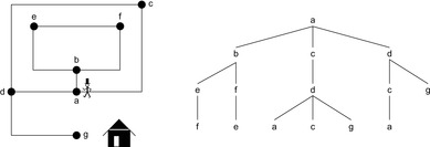
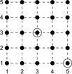
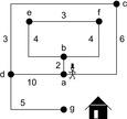
The set of all explicitly generated paths rooted at the start node and of which the leaves are the Open nodes constitutes the search tree of the underlying problem graph. Note that while the problem graph is defined solely by the problem domain description, the search tree characterizes the part explored by a search algorithm at some snapshot during its execution time. Figure 2.1 gives a visualization of a problem graph and a corresponding search tree.
 |
| Figure 2.1 |
In tree-structured problem spaces, each node can only be reached on a single path. However, it is easy to see that for finite acyclic graphs, the search tree can be exponentially larger than the original search space. This is due to the fact that a node can be reached multiple times, at different stages of the search via different paths. We call such a node a duplicate; for example, in Figure 2.1 all shown leaves at depth 3 are duplicates. Moreover, if the graph contains cycles, the search tree can be infinite, even if the graph itself is finite.
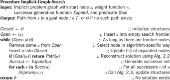
In Algorithm 2.1 we sketch a framework for a general node expansion search algorithm.
Definition 2.1
(Closed/Open Lists) The set of already expanded nodes is called Closed and the set of generated but yet unexpanded nodes is called Open. The latter is also denoted as the search frontier.
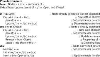
As long as no solution path has been established, a frontier node u in Open is selected and its successors are generated. The successors are then dealt with in the subroutine Improve, which updates Open and Closed accordingly (in the simplest case, it just inserts the child node into Open). At this point, we deliberately leave the details of how to Select and Improve a node unspecified; their subsequent refinement leads to different search algorithms.
Open and Closed were introduced as data structures for sets, offering the opportunities to insert and delete nodes. Particularly, an important role of Closed is duplicate detection. Therefore, it is often implemented as a hash table with fast lookup operations.
Duplicate identification is total, if in each iteration of the algorithm, each node in Open and Closed has one unique representation and generation path. In this chapter, we are concerned with algorithms with total duplicate detection. However, imperfect detection of already expanded nodes is quite frequent in state space search out of necessity, because very large state spaces are difficult to store with respect to given memory limitations. We will see many different solutions to this crucial problem in upcoming chapters.
Generation paths do not have to be fully represented for each individual node in the search tree. Rather, they can be conveniently stored by equipping each node u with a predecessor link  , which is a pointer to the parent in the search tree (or
  for the root s). More formally,
  if
if  . By tracing the links back in bottom-up direction until we arrive at the root s, we can reconstruct a solution path
  of length k as
  (see Alg. 2.2).
Algorithm 2.3 sketches an implementation of Improve with duplicate detection and predecessor link updates. 1 Note that this first, very crude implementation does not attempt to find a shortest path; it merely decides if a path exists at all from the start node to a goal node.
1In this chapter we explicitly state the calls to the underlying data structure, which are considered in detail Chapter 3. In later chapters of the book we prefer sets for Open and Closed.
To illustrate the behavior of the search algorithms, we take a simple example of searching a goal node at  from node
  in the Gridworld of Figure 2.2. Note that the potential set of paths of length i in a grid grows exponentially in i; for
  we have at most
  , for
, for  we have at most
  , and for
  we have at most
  paths.
2.1.1. Depth-First Search
For depth-first search (DFS), the Open list is implemented as a stack (a.k.a. a LIFO, or last-in first-out queue), so that Insert is in fact a push operation and Select corresponds to a pop operation. Operation push places an element and operation pop extracts an element at the top of this data structure. Successors are simply pushed onto the stack. Thus, each step greedily generates a successor of the last visited node, unless it has none, in which case it backtracks to the parent and explores another not yet explored sibling.
It is easy to see that in finite search spaces DFS is complete (i.e., will find a solution path if there is some), since each node is expanded exactly once. It is, however, not optimal. Depending on which successor is expanded first, any path is possible. Take, for example, the solution ((3,3), (3,2), (2,2), (2,3), (2,4), (2,5), (3,5), (3,4), (4,4), (4,3), (5,3), (5,4), (5,5)) in the Gridworld example. The path length, defined as the number of state transitions, is 12 and hence larger than the minimum.
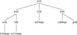
Table 2.1 and Figure 2.3 show the expansion steps and the search tree explored by DFS when run on the example of Figure 2.1. Without loss of generality, we assume that children are expanded in alphabetical order.
| Step | Selection | Open | Closed | Remarks |
|---|---|---|---|---|
| 1 | {} | {a} | {} | |
| 2 | a | {b,c,d} | {a} | |
| 3 | b | {e,f,c,d} | {a,b} | |
| 4 | e | {f,c,d} | {a,b,e} | f is duplicate |
| 5 | f | {c,d} | {a,b,e,f} | e is duplicate |
| 6 | c | {d} | {a,b,e,f,c} | d is duplicate |
| 7 | d | {g} | {a,b,e,f,c,d} | c is duplicate |
| 8 | g | {} | {a,b,e,f,c,d,g} | Goal reached |
 |
| Figure 2.3 DFS search tree for the example in Figure 2.1. The numbers in brackets denote the order of node generation. |
Without duplicate elimination, DFS can get trapped in cycles of the problem graph and loop forever without finding a solution at all.
2.1.2. Breadth-First Search
For breadth-first search (BFS), the set Open is realized as a first-in first-out queue (FIFO). The Insert operation is called Enqueue, and adds an element to the end of the list; the Dequeue operation selects and removes its first element. As a result, the neighbors of the source node are generated layer by layer (one edge apart, two edges apart, and so on).
As for DFS, Closed is implemented as a hash table, avoiding nodes to be expanded more than once. Since BFS also expands one new node at a time, it is complete in finite graphs. It is optimal in uniformly weighted graphs (i.e., the first solution path found is the shortest possible one), since the nodes are generated in level order with respect to the tree expansion of the problem graph.
One BFS search order in the Gridworld example is ((3,3), (3,2), (2,3), (4,3), (3,4), (2,2), (4,4), (4,2), (2,4), (3,5), (5,3), (1,3), (3,1), …, (5,5)). The returned solution path ((3,3), (4,3), (4,4), (4,5), (5,5)) is optimal.
| Step | Selection | Open | Closed | Remarks |
|---|---|---|---|---|
| 1 | {} | {a} | {} | |
| 2 | a | {b,c,d} | {a} | |
| 3 | b | {c,d,e,f} | {a,b} | |
| 4 | c | {d,e,f} | {a,b,c} | d is duplicate |
| 5 | d | {e,f,g} | {a,b,c,d} | c is duplicate |
| 6 | e | {f,g} | {a,b,c,d,e} | f is duplicate |
| 7 | f | {g} | {a,b,c,d,e,f} | e is duplicate |
| 8 | g | {} | {a,b,c,d,e,f,g} | Goal reached |
 |
| Figure 2.4 BFS search tree for the example in Figure 2.1. The numbers in brackets denote the order of node generation. |
A possible drawback for BFS in large problem graphs is its large memory consumption. Unlike DFS, which can find goals in large search depth, it stores all nodes with depth smaller than the shortest possible solution length.
2.1.3. Dijkstra's Algorithm
So far we have looked at uniformly weighted graphs only; that is, each edge counts the same. Now let us consider the generalization that edges are weighted with a weight function (a.k.a. cost function) w. In weighted graphs, BFS loses its optimality. Take, for example, weights on the DFS solution path p of 1/12, and weights of 1 for edges not on p. This path is of total weight 1, and the BFS solution path is of weight  .
.
To compute the shortest (cheapest) path in graphs with nonnegative weights, Dijkstra proposed a greedy search strategy based on the principle of optimality. It states that an optimal path has the property that whatever the initial conditions and control variables (choices) over some initial period, the control (or decision variables) chosen over the remaining period must be optimal for the remaining problem, with the node resulting from the early decisions taken to be the initial condition. Applying the principle developed by Richard Bellman to shortest path search results in In words, the minimum distance from s to v is equal to the minimum of the sum of the distance from s to a predecessor u of v, plus the edge weight between u and v. This equation implies that any subpath of an optimal path is itself optimal (otherwise it could be replaced to yield a shorter path).
The search algorithm maintains a tentative value of the shortest distance. More precisely, an upper bound  on
on  for each node u; initially set to
  ,
,  is successively decreased until it matches
  . From this point on, it remains constant throughout the rest of the algorithm.
A suitable data structure for maintaining Open is a priority queue, which associates each element with its f-value, and provides operations Insert and DeleteMin (accessing the element with the minimum f-value and simultaneously removing it from the priority queue). Additionally, the DecreaseKey operation can be thought of as deleting an arbitrary element and reinserting it with a lower associated f-value; executing these two steps together can be performed more efficiently in some implementations. Note that the signature of Insert requires now an additional parameter: the value used to store the node in the priority queue.
The algorithm initially inserts s into the priority queue with  set to zero. Then, in each iteration an Open node u with minimum f-value is selected, and all its children v reachable by outgoing edges are generated. The subroutine Improve of Algorithm 2.1 now updates the stored estimate
  for v if the newly found path via u is shorter than the best previous one. Basically, if for a path you can take a detour via another path to shorten the path, then it should be taken. Improve inserts v into Open, in turn. The pseudo code is listed in Algorithm 2.4. This update step is also called a node relaxation. An example is given in Figure 2.5.
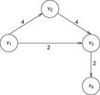
For illustration, we generalize our running example by assuming edge weights, as given in Figure 2.6. The execution of the algorithm is given in Table 2.3 and Figure 2.7.
 |
| Figure 2.6 Extended example in Figure 2.1 with edge weights. |
| Step | Selection | Open | Closed | Remarks |
|---|---|---|---|---|
| 1 | {} | {a(0)} | {} | |
| 2 | a | {b(2),c(6),d(10)} | {a} | |
| 3 | b | {e(6),f(6),c(6),d(10)} | {a,b} | Ties broken arbitrarily |
| 4 | e | {f(6),c(6),d(10)} | {a,b,e} | f is duplicate |
| 5 | f | {c(6),d(10)} | {a,b,e,f} | e is duplicate |
| 6 | c | {d(9)} | {a,b,e,f} | d reopened, parent changes to c |
| 7 | d | {g(14)} | {a,b,e,f,c,d} | a is duplicate |
| 8 | g | {} | {a,b,e,f,c,d,g} | Goal reached |
 |
| Figure 2.7 Single-Source Shortest Paths search tree for the example in Figure 2.6. The numbers in brackets denote the order of node generation/f-value. |
The correctness argument of the algorithm is based on the fact that for a node u with minimum f-value in Open, f is exact; that is,  .
.
Lemma 2.1
(Optimal Node Selection) Let  be a positively weighted graph and f be the approximation of
  in Dijkstra's algorithm. At the time u is selected in the algorithm, we have
  .
.
Proof
Assume the contrary and let u be the first selected node from Open with  ; that is,
  . Furthermore, let
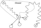
  be a shortest path for u with y being the first node on the path that is not expanded (see Fig. 2.8).
It is important to observe that Lemma 2.1 suits Dijkstra's exploration scheme to implicit enumeration, because at the first encountering of a goal node t we already have  .
.
Theorem 2.1
(Correctness Dijkstra's Algorithm) In weighted graphs with nonnegative weight function the algorithm of Dijkstra's algorithm is optimal; that is, at the first node  that is selected for expansion, we have
  .
.
Proof
With nonnegative edge weights, for each pair  with
with  we always have
  . Therefore, the values f for selected nodes are monotonically increasing. This proves that at the first selected node
  we have
  .
.
In infinite graphs we have to guarantee that a goal node will eventually be reached.
Theorem 2.2
(Dijkstra's Algorithm on Infinite Graphs) If the weight function w of a problem graph  is strictly positive and if the weight of every infinite path is infinite, then Dijkstra's algorithm terminates with an optimal solution.
Proof
The premises induce that if the cost of a path is finite, the path itself is finite. Therefore, there are only finitely many paths of cost smaller than  . We further observe that no path of cost
  can be a prefix of an optimal solution path. Therefore, Dijkstra's algorithm examines the problem graph only on a finite subset of all infinite paths. A goal node
  with
with  will eventually be reached, so that Dijkstra's algorithm terminates. The solution will be optimal by the correctness argument of Theorem 2.1.
Note that for all nodes u in Closed, an optimal path from s to u has been found. Thus, a slight modification of Dijkstra's algorithm that only stops when Open runs empty can not only find the shortest path between a single source s and a single target t, but also to all other nodes (provided, of course, that the number of nodes is finite).
2.1.4. Negatively Weighted Graphs
Unfortunately, the correctness and optimality argument in Lemma 2.1 is no longer true for graphs with negative edge weights. As a simple example, consider the graph consisting of three nodes  having edges
  with
with  ,
,  with
with  , and edge
  with
with  , for which the algorithm of Dijkstra computes
  instead of the correct value,
  .
.
An even worse observation is that negatively weighted graphs may contain negatively weighted cycles, so that the shortest path may be infinitely long and of value  . This has led to the Bellman-Ford algorithm to be described later. However, we can still handle graphs with negative weights using a modified Dijkstra algorithm if we impose a slightly less restrictive condition on the graph, namely that
  for all u. That is, the distance from each node to the goal is nonnegative. Figuratively speaking, we can have negative edges when far from the goal, but they get “eaten up” when coming closer. The condition implies that no negatively weighted cycles exist.
In the sequel, we will denote the extended version of Dijkstra's algorithm as algorithm A. As can be gleaned from the comparison between Algorithm 2.5 and Algorithm 2.4, with negative edges it can be necessary to reopen not only Open nodes, but also Closed ones.
Lemma 2.2
(Invariance for Algorithm A) Let  be a weighted graph,
  be a least-cost path from the start node s to a goal node
  , and f be the approximation in the algorithm A. At each selection of a node u from Open, we have the following invariance:
(I) Unless  is in Closed with
  , there is a node
  in Open such that
  , and no
  exists such that
  is in Closed with
  .
.
Proof
Without loss of generality let i be maximal among the nodes satisfying (I). We distinguish the following cases:
1. Node u is not on p or  . Then node
  remains in Open. Since no v in
  with
with  is changed and no other node is added to Closed, (I) is preserved.
2. Node u is on p and  . If
. If  , there is nothing to show.
First assume  . Then Improve will be called for
  ; for all other nodes in
  , the argument of case 1 holds. According to (I), if v is in Closed, then
  , and it will be reinserted into Open with
  . If v is neither in Open nor Closed, it is inserted into Open with this merit. Otherwise, the DecreaseKey operation will set it to
  . In either case, v guarantees the invariance (I).
Now suppose  . By the maximality assumption of i we have
  with
with  . If
. If  , no DecreaseKey operation can change it because
  already has optimal merit
  . Otherwise,
  remains in Open with an unchanged f-value and no other node besides u is inserted into Closed; thus,
  still preserves (I).
Theorem 2.3
(Correctness of Algorithm A) Let  be a weighted graph so that for all u in V we have
  . Algorithm A is optimal; that is, at the first extraction of a node t in T we have
  .
.
Proof
Assume that the algorithm does terminate at node  with
with  . According to
  there is a node u with
  in Open, which lies on an optimal solution path
  to t. We have
 in contradiction to the fact that
  is selected from Open.
In infinite graphs we can essentially apply the proof of Theorem 2.2.
Theorem 2.4
(A in Infinite Graphs) If the weight of every infinite path is infinite, then algorithm A terminates with an optimal solution.
Proof
Since  for all u, no path of cost
  can be a prefix of an optimal solution path.
2.1.5. Relaxed Node Selection
Dijkstra's algorithm is bound to always expand an Open node with minimum f-value. However, as we will see in later chapters, sometimes it can be more efficient to choose nodes based on other criteria. For example, in route finding in large maps we might want to explore neighboring streets in subregions together to optimize disk access.
In Algorithm 2.6 we give a pseudo-code implementation for a relaxed node selection scheme that gives us precisely this freedom. In contrast to Algorithm A and Dijkstra's algorithm, reaching the first goal node will no longer guarantee optimality of the established solution path. Hence, the algorithm has to continue until the Open list runs empty. A global current best solution path length U is maintained and updated; the algorithm improves the solution quality over time.
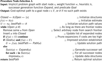
If we want the algorithm to be optimal we have to impose the same restriction on negatively weighted graphs as in the case of Algorithm A.
Theorem 2.5
(Optimality Node-Selection A, Conditioned) If we have  for all nodes
  , then node selection A terminates with an optimal solution.
Proof
Upon termination, each node inserted into Open must have been selected at least once. Suppose that invariance (I) is preserved in each loop; that is, that there is always a node v in the Open list on an optimal path with  . Thus, the algorithm cannot terminate without eventually selecting the goal node on this path, and since by definition it is not more expensive than any found solution path and best maintains the currently shortest path, an optimal solution will be returned. It remains to show that the invariance (I) holds in each iteration. If the extracted node u is not equal to v there is nothing to show. Otherwise,
  . The bound U denotes the currently best solution length. If
  , no pruning takes place. On the other hand,
  leads to a contradiction since
  (the latter inequality is justified by
  ).
).
If we do allow  to become negative, we can at least achieve the following optimality result.
Theorem 2.6
(Optimality Node-Selection A, Unconditioned) For 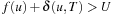 -as the pruning condition in the node selection A algorithm, it is optimal.
Proof
By analogy to the previous theorem, it remains to show that (I) holds in each iteration. If the extracted node u is not equal to v there is nothing to show. Otherwise,  . The bound U denotes the currently best solution length. If
 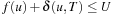 , no pruning takes place. On the other hand,
  leads to a contradiction since
  , which is impossible given that U denotes the cost of some solution path; that is,
  .
.
Unfortunately, we do not know the value of  , so the only thing that we can do is to approximate it; in other words, to devise a bound for it.
2.1.6. * Algorithm of Bellman-Ford
Bellman and Ford's algorithm is the standard alternative to Dijkstra's algorithm when searching graphs with negative edge weights. It can handle any such finite graphs (not just those with nonnegative goal distances), and will detect if negative cycles exist.
The basic idea of the algorithm is simple: relax all edges in each of  passes (n is the number of nodes in the problem graph), where node relaxation of edge
  is one update of the form
  . It satisfies the invariant that in pass i, all cheapest paths have been found that use at most
  edges. In a final pass, each edge is checked once again. If any edge can be further relaxed at this point, a negative cycle must exist; the algorithm reports this and terminates. The price we pay for the possibility of negative edges is a time complexity of
  , worse than Dijkstra's algorithm by a factor of
  .
.
Most of the time, the Bellman-Ford algorithm is described in terms of explicit graphs, and is used to compute shortest paths from a source to all other nodes. In the following, however, we develop an implicit version of the algorithm of Bellman and Ford that makes it comparable to the previously introduced algorithms. One advantage is that we can exploit the fact it is necessary to perform this relaxation in iteration i only if the f-value of u has changed in iteration  .
.
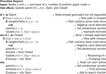
Note that the Bellman-Ford algorithm can be made to look almost identical to Dijkstra's algorithm by utilizing a queue instead of a priority queue: For all nodes u extracted from one end of the queue, relax every successor v of u, and insert v into the tail of the queue. The reasoning is as follows. For graphs with negative edge weights it is not possible to have perfect choice on the extracted element that is known to be contained in the Open list by invariance (I) (see page 58). As we have seen, considering already expanded nodes is necessary. Suppose that u is the extracted node. Before u is selected for next time the optimal node  with
with  has to be selected at least once, such that the solution path
  that is associated with
  is extended by at least one edge. To implement this objective for convenience we redisplay the Improve procedure that has been devised so far for the situation where the Open list is a queue. Algorithm 2.7 shows the pseudo code.
The implicit version of Bellman and Ford is listed in Algorithm 2.8. In the original algorithm, detection of negative cycles is accomplished by checking for optimal paths longer than the total number of nodes, after all edges have been relaxed  times. In our implicit algorithm, this can be done more efficiently. We can maintain the length of the path, and as soon as any one gets longer than n, we can exit with a failure notice. Also, more stringent checking for duplicates in a path can be implemented.
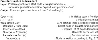
We omitted the termination condition at a goal node, but it can be implemented analogously as in the node selection A algorithm. That is, it is equivalent whether we keep track of the current best solution during the search or (as in the original formulation) scan all solutions after completion of the algorithm.
Theorem 2.7
(Optimality of Implicit Bellman-Ford) Implicit Bellman-Ford is correct and computes optimal cost solution paths.
Proof
Since the algorithm only changes the ordering of nodes that are selected, the arguments for the correctness and optimality of the implicit version of Bellman and Ford's and the node selection A algorithm are the same.
Theorem 2.8
(Complexity of Implicit Bellman-Ford) Implicit Bellman-Ford applies no more than O(ne) node generations.
Proof
Let  be the set Open (i.e., the content of the queue) when u is removed for the i th time from Open. Then, by applying the Invariant (I) (Lemma 2.2) we have that
  contains at least one element, say
  , with optimal cost. Since Open is organized as a queue,
  is deleted from Open before u is deleted for the
  -th time. Since
  is on the optimal path and will never be added again, we have the number of iterations i is smaller than the number of nodes in the expanded problem graph. This proves that each edge is selected at most n times, so that at most ne nodes are generated.
2.1.7. Dynamic Programming
The divide-and-conquer strategy in algorithm design suggests to solve a problem recursively by splitting it into smaller subproblems, solving each of them separately, and then combining the partial results into an overall solution. Dynamic programming was invented as a similarly general paradigm. It addresses the problem that a recursive evaluation can give rise to solving overlapping subproblems repeatedly, invoked for different main goals. It suggests to store subresults in a table so that they can be reused. Such a tabulation is most efficient if an additional node order is given that defines the possible subgoal relationships.
All Pair Shortest Paths
For example, consider the problem of finding the shortest distance for each pair of nodes in  . We could run either Single-Source Shortest Paths algorithms discussed so far—BFS or Dijkstra's algorithm—repeatedly, starting from each node i in turn, but this would traverse the whole graph several times. A better solution is to apply the All Pairs Shortest Paths Floyd-Warshall algorithm. Here, all distances are recorded in an n-by-n matrix D, where element
  indicates the shortest path costs from i to j. A sequence of matrices
  is computed, where
  contains only the edge weights (it is the adjacency matrix), and
  contains the shortest distances between nodes with the constraint that intermediate nodes have no index larger than k.
According to the principle of optimality it holds that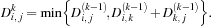 In particular, if no path between i and j passes through k, then
  . Algorithm 2.9 solves the All Pairs Shortest Paths problem in
  time and
  space.

Multiple Sequence Alignment
Dynamic programming is a very effective means in many domains. Here, we will give a Multiple Sequence Alignment example (see Sec. 1.7.6). Let w define the cost of substituting one character with another, and denote the distance between two strings  and
and  as
as  . Then, according to the principle of optimality, the following recurrence relation holds:
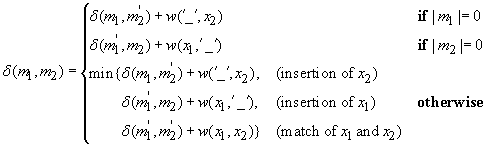
A pairwise alignment can be conveniently depicted as a path between two opposite corners in a two-dimensional grid: one sequence is placed on the horizontal axis from left to right, the other one on the vertical axis from top to bottom. If there is no gap in either string, the path moves diagonally down and right; a gap in the vertical (horizontal) string is represented as a horizontal (vertical) move right (down), since a letter is consumed in only one of the strings. The alignment graph is directed and acyclic, where a (nonborder) vertex has incoming edges from the left, top, and top-left adjacent vertices, and outgoing edges to the right, bottom, and bottom-right vertices.
The algorithm progressively builds up alignments of prefixes of m and  in a bottom-up fashion. The costs of partial alignments are stored in a matrix D, where
  contains the distance between
  and
and  . The exact order of the scan can vary (e.g., rowwise or columnwise), as long as it is compatible with a topological order of the graph; a topological order of a directed, acyclic graph is a sorting of the nodes
  , such that if
  is reachable from
  , then it must hold that
  . In particular,
  has no incoming edges, and if the number of nodes is some finite n, then
  has no outgoing edges. In general, many different topological orderings can be constructed for a given graph.
For instance, in the alignment of two sequences, a cell value depends on the values of the cells to the left, top, and diagonally top-left, and these have to be explored before it. Algorithm 2.10 shows the case of columnwise traversal. Another particular such ordering is that of antidiagonals, which are diagonals running from top-right to bottom-left. The antidiagonal number of a node is simply the sum of its coordinates.
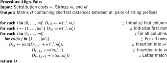
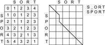
As an example, the completed matrix for the edit distance between the strings sport and sort is shown in Figure 2.9. After all matrix entries have been computed, the solution path has to be reconstructed to obtain the actual alignment. This can be done iteratively in a backward direction starting from the bottom-right corner up to the top-left corner, and selecting in every step a parent node that allows a transition with the given cost. Alternatively, we could store in each cell an additional pointer to the relevant predecessor.
It is straightforward to generalize pairwise sequence alignment to the case of aligning k sequences simultaneously, by considering higher-dimensional lattices. For example, an alignment of three sequences can be visualized as a path in a cube. Figure 2.10 illustrates an example for the alignment
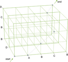
A B C _ B
_ B C D _
_ _ _ D B
If the sequence length is at most n, the generalization of Algorithm 2.10 requires  time and space to store the dynamic programming table. In Section 6.3.2, we will present a refined algorithm that reduces the space complexity by one order of magnitude. 2 An example of how successor costs are calculated, with the cost matrix of Figure 2.10 and a gap opening penalty of 4, is shown in Figure 2.11.
2As a technical side note, we remark that to deal with the biologically more realistic affine gap costs, we can no longer identify nodes in the search graph with lattice vertices; this is because the cost associated with an edge depends on the preceding edge in the path. Similarly, as in route planning with turn restrictions, in this case, it is more suitable to store lattice edges in the priority queue, and let the transition costs for  be the sum-of-pairs substitution costs for using one character from each sequence or a gap, plus the incurred gap penalties for
  followed by
  . Note that the state space in this representation grows by a factor of
  .
.
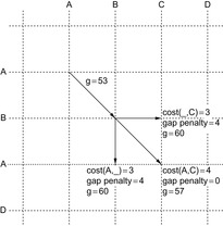 |
| Figure 2.11 Example of computing path costs with affine gap function; the substitution matrix of Figure 2.10 and a gap opening penalty of 4 is used. |
Markov Decision Process Problems
A common way of calculating an optimal policy is by means of dynamic programming using either policy iteration or value iteration.
Both policy iteration and value iteration are based on the Bellman optimality equation,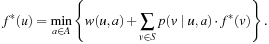
In some cases, we apply a discount  to handle infinite paths. Roughly speaking, we can define the value of a state as the total reward/cost an agent can expect to accumulate when traversing the graph according to its policy, starting from that state. The discount factor defines how much more we should value immediate costs/rewards, compared to costs/rewards that are only attainable after two or more steps. Formally, the corresponding equation according to the principle of optimality is
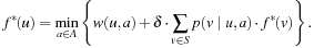 Policy iteration successively improves a policy
  by setting
 for each state u, where the evaluation of
  ,
,  , can be computed as a system of
  linear equations:
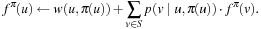 A pseudo-code implementation for policy iteration is shown in Algorithm 2.11.
Value iteration improves the estimated cost-to-go function f by successively performing the following operation for each state u: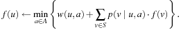 The algorithm exits if an error bound on the policy evaluation falls below a user-supplied threshold ϵ, or a maximum number of iterations have been executed. If the optimal cost
  is known for each state, the optimal policy can be easily extracted by choosing an operation according to a single application of the Bellman equation. Value iteration is shown in pseudo code in Algorithm 2.12. The procedure takes a heuristic h for initializing the value function as an additional parameter.
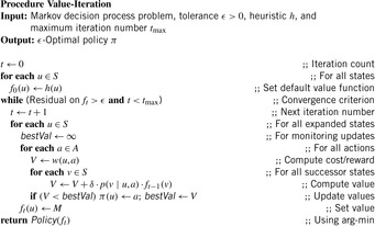
The error bound on the value function is also called the residual, and can, for example, be computed in form  . A residual of zero denotes that the process has converged. An advantage of policy iteration is that it converges to the exact optimum, whereas value iteration usually only reaches an approximation. On the other hand, the latter technique is usually more efficient on large state spaces.
For implicit search graphs the algorithms proceed in two phases. In the first phase, the whole state space is generated from the initial state s. In this process, an entry in a hash table (or vector) is allocated to store the f-value for each state u; this value is initialized to the cost of u if  , or to a given (not necessarily admissible) heuristic estimate (or zero if no estimate is available) if u is nonterminal. In the second phase, iterative scans of the state space are performed updating the values of nonterminal states u as
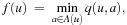 where
where  , which depends on the search model (see Sec. 1.8.4).
(2.1)
Value iteration converges to the solution optimal value function provided that its values are finite for all  . In the case of MDPs, which may have cyclic solutions, the number of iterations is not bounded and value iteration typically only converges in the limit. For this reason, for MDPs, value iteration is often terminated after a predefined bound of
  iterations are performed, or when the residual falls below a given ϵ > 0.
Monte Carlo policy evaluation estimates  , the value of a state under a given policy. Given a set of iterations, value
  is approximated by following
  . To estimate
  , we count the visits to a fixed state u. Value
  is computed by averaging the returns in a set of iterations. Monte Carlo policy evaluation converges to
  as the number of visits goes to infinity. The main argument is that by the law of large numbers the sequence of averages will converge to their expectation.
For convenience of terminology, in the sequel we will continue referring to nodes when dealing with the search algorithm.
2.2. Informed Optimal Search
We now introduce heuristic search algorithms; that is, algorithms that take advantage of an estimate of the remaining goal distance to prioritize node expansion. Domain-dependent knowledge captured in this way can greatly prune the search tree that has to be explored to find an optimal solution. Therefore, these algorithms are also subsumed under the category informed search.
2.2.1. A*
The most prominent heuristic search algorithm is A*. It updates estimates  (a.k.a. merits) defined as
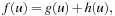 where
where  is the weight of the (current optimal) path from s to u, and
  is an estimate (lower bound) of the remaining costs from u to a goal, called the heuristic function. Hence, the combined value
  is an approximation for the cost of the entire solution path (see Fig. 2.12). For the sake of completeness, the entire algorithm is shown in Algorithm 2.13.
For illustration, we again generalize our previous example by assuming that we can obtain heuristic estimates from an unknown source, as shown in Figure 2.13. The execution of the A* algorithm is given in Table 2.4 and Figure 2.14, respectively. We see that compared to Dijkstra's algorithm, nodes  and f can be pruned from expansion since their f-value is larger than the cheapest solution path.
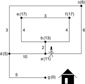 |
| Figure 2.13 Extended example of Figure 2.6 with heuristic estimates (in parentheses). |
| Step | Selection | Open | Closed | Remarks |
|---|---|---|---|---|
| 1 | {} | {a(0,11)} | {} | |
| 2 | a | {c(6,14),b(2,15),d(10,15)} | {a} | |
| 3 | c | {d(9,14),b(2,15)} | {a,c} | update d, change parent to c |
| 4 | d | {g(14,14),b(2,15)} | {a,c,d} | a is duplicate |
| 5 | g | {b(2,15)} | {a,c,d,g} | goal reached |
 |
| Figure 2.14 A* search tree for the example of Figure 2.13. The numbers in parentheses denote the order of node generation / h-value, f-value. |
The attentive reader might have noticed our slightly sloppy notation in Algorithm 2.13: We use the term  in the Improve procedure, however, we don't initialize these values. This is because in light of an efficient implementation, it is necessary to store either the g-value or the f-value of a node, but not both. If only the f-value is stored, we can derive the f-value of node v with parent u as
  .
.
By following this reasoning, it turns out that algorithm A* can be elegantly cast as Dijkstra's algorithm in a reweighted graph, where we incorporate the heuristic into the weight function as  An example of this reweighting transformation of the implicit search graph is shown in Figure 2.15. One motivation for this transformation is to inherit correctness proofs, especially for graphs. Furthermore, it bridges the world of traditional graphs with an AI search. As a by-product, the influence heuristics have is clarified. Let us formalize this idea.
Lemma 2.3
Let G be a weighted problem graph and  . Define the modified weight
  as
as  . Let
. Let  be the length of the shortest path from s to t in the original graph and
  be the corresponding value in the reweighted graph.
1. For a path p, we have  , if and only if
  .
.
2. Moreover, G has no negatively weighted cycles with respect to w if and only if it has none with respect to  .
.
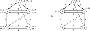
As an example, consider the two graphs in Figure 2.16. To the left the original problem graph with heuristic estimates attached to each node is shown. Each node u is additionally labeled by the value  . In the reweighted graph to the right the computed f-values after expanding node s are shown. The inconsistency on the original graph on edge
  generates a negative weight in the reweighted graph.
The usual approach to deal with inconsistent but admissible heuristics in the context of A* is called pathmax. It takes the maximum of the accumulated weights on the path to a node to enforce a monotone growth in the cost function. More formally for a node u with child v the pathmax equation sets  to
to  or, equivalently,
  to
to  , such that h does not overestimate the distance from the parent to the goal.
The approach is wrong if we apply its reasoning to a graph search as A*. In the example in Figure 2.16, after expanding nodes s and a we have  and
and  . Now a is reached once more via b by means
  , it is moved to Closed, and
  is compared to the closed list. We have that 12 is the pathmax on path
  . Wrongly we keep
  and all information contained in
  is lost forever.
The equation  is equivalent to
  . A consistent heuristic yields a first A* variant of Dijkstra's algorithm.
Theorem 2.9
(A* for Consistent Heuristics) Let h be consistent. If we set  for the initial node s and update
  with
with  instead of
  , at each time a node
  is selected, we have
  .
.
Proof
Since h is consistent, we have  . Therefore, the preconditions of Theorem 2.1 are fulfilled for weight function
  , so that
  , if u is selected from Open. According to Lemma 2.3, shortest paths remain invariant through reweighting. Hence, if
  is selected from Open we have
 Since
Since  , we have
  for all successors v of u. The f-values increase monotonically so that at the first extraction of
  we have
  .
.
In case of negative values for  , shorter paths to already expanded nodes may be found later in the search process. These nodes are reopened.
In the special case of unit edge cost and trivial heuristic (i.e.,  for all u), A* proceeds similarly to the breadth-first search algorithm. However, the two algorithms can have different stopping conditions. BFS stops as soon as it generates the goal. A* will not stop–it will insert the goal in the priority queue and it will finish level
  before it terminates (assuming the goal is at distance d from the start node). Therefore, the difference between the two algorithms can be as large as the number of nodes at level
  , which is usually a significant fraction (e.g., half) of the total number of nodes expanded. The reason BFS can do this and A* cannot is because the stopping condition for BFS is correct only when all the edge weights in the problem graph are the same. A* is general-purpose–it has to finish level
  because there might be an edge leading to the goal of which the edge has value 0, leading to a better solution. There is an easy solution to this. If node u is adjacent to a goal node then define
  . The new weight of an optimal edge is 0 so that it is searched first.
Lemma 2.4
Let G be a weighted problem graph, h be a heuristic, and  . If h is admissible, then
  .
.
Proof
Since  and since the shortest path costs remain invariant under reweighting of G by Lemma 2.3, we have
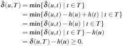
Theorem 2.10
(A* for Admissible Heuristics) For weighted graphs  and admissible heuristics h, algorithm A* is complete and optimal.
Proof
Immediate consequence of Lemma 2.4 together with applying Theorem 2.3.
A first remark concerning notation: According to the original formulation of the algorithm, the  in
in  ,
,  ,
,  , and so on was used to denote optimality. As we will see, many algorithms developed later were named conforming to this standard. Do not be surprised if you see many stars!
With respect to the search objective  , Figure 2.17 illustrates the effect of applying DFS, BFS, A*, and greedy best-first search, the A* derivate with
  .
.

2.2.2. On the Optimal Efficiency of A*
It is often said that A* does not only yield an optimal solution, but that it expands the minimal number of nodes (up to tie breaking). In other words, A* has optimal efficiency for any given heuristic function, or no other algorithm can be shown to expand fewer nodes than A*. The result, however, is only partially true. It does hold for consistent heuristics, but not necessarily for admissible heuristics. We first give a proof for the first case and a counterexample for the second one.
Consistent Heuristics
We remember that we can view a search with a consistent heuristic as a search in a reweighted problem graph with nonnegative costs.
Theorem 2.11
(Efficiency Lower Bound) Let G be a problem graph with nonnegative weight function, with initial node s and final node set T, and let  be the optimal solution cost. Any optimal algorithm has to visit all nodes
  with
with  .
.
Proof
We assume the contrary; that is, that an algorithm A finds an optimal solution  with
with  and leaves some u with
  unvisited. We will show that there might be another solution path q with
  that is not found. Let
  be the path with
  , let t be a supplementary special node in T and V, and let
  be a new edge with
  . Since u is not expanded, for A we do not know if
  exists. Let
  . Then
If the values  are pairwise different, then there is no tie, and the number of nodes that A expands will have to be larger than or equal to the number of nodes that A* expands.
Nonconsistent Heuristics
If we have admissibility but not consistency, A* will reopen nodes. Even worse, as we will indicate later, A* might reopen nodes exponentially many times, even if the heuristic is admissible. This leads to an exponential time consumption in the size of the graph. Fortunately, this strange behavior does not appear frequently in practice, as in most cases we deal with unit costs, limiting the number of possible improvements for a particular node to the depth of the search.
Based on the process of reweighting edges, we can better reflect what happens when we reopen nodes. If we consider nonconsistent heuristics, the reweighted problem graph may contain negative edges. If we consider  as the new edge costs, Figure 2.18 gives an example for a problem graph that leads to exponentially many reopenings. The second last node is reopened for every path with weight
  .
.
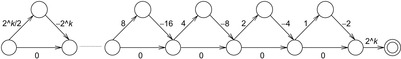
It is not difficult to restore a heuristic function with nonnegative edge costs. For the top-level nodes in the triangles we have  , …, 24, 12, 6, and 3, and for the bottom level node we have
  ,
,  , 8, 4, 2, 1, and 0. The weights for the in- and outgoing edges at the top-level nodes are zero, and the bottom-level edges are weighted
  , …, 8, 4, 2, 1, and
  .
.
Recourse to basic graph theory shows that there are algorithms that can do better. First of all, we notice that the problem graph structure is directed and acyclic so that a linear-time algorithm relaxes the nodes in topological order. General problem graphs with negative weights are dealt with by the algorithm of Bellman and Ford (see Alg. 2.8), which has a polynomial complexity. But even if we call the entire algorithm of Bellman and Ford for every expanded node, we have an accumulated complexity of  , which is large but not exponential as with A* and reopening. As a consequence, the efficiency of A* is not optimal. Nonetheless, in the domains that are used in problem solving practice, reopenings are rare, so that A*'s strategy is still a good choice. One reason is that for bounded weights, the worst-case number of reopenings is polynomial.
2.3. *General Weights
Next we consider generalizing the state space search by considering an abstract notion of costs. We will consider optimality with respect to a certain cost or weight associated to edges. We abstract costs by an algebraic formalism and adapt the heuristic search algorithms accordingly. We first define the cost algebra we are working on. Then we turn to a cost-algebraic search in graphs, in particular for solving the optimality problem. Cost-algebraic versions of Dijkstra's algorithm and A* with consistent and admissible estimates are discussed. Lastly we discuss extensions to a multiobjective search.
2.3.1. Cost Algebras
Cost-algebraic search methods generalize edge weights in a rather straightforward way to more general cost structures. Our formalism for cost is called cost algebra. We recall some required definitions of algebraic concepts.
Let A be a set and  be a binary action. A monoid is a tuple
  if
if  and for all
  ,
,
Intuitively, set A will represent the domain of the costs and × is the operation representing the cumulation of costs.
Let A be a set. A relation  is a total order whenever for all
  ,
,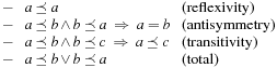
We write  if
if  and
and  . We say that a set A is isotone if
  implies both
  and
and  for all
  .
.
Definition 2.2
(Cost Algebra) A cost algebra is a 5-tuple  , such that
  ,
,  ,
,  , and
, and  .
.
The least and greatest operations are defined as follows:  such that
  for all
  , and
, and  such that
  for all
  .
.
Intuitively, A is the domain set of cost values, × is the operation used to cummulate values and  is the operation used to select the best (the least) among values. Consider, for example, the following cost algebras:
•  (optimization)
•  (max/min)
The only nontrivial property to be checked is isotonicity.
Not all algebras are isotone; for example, take  with
with  and
and  if
if  or
or  if
if  . We have
  but
but  . However, we may easily verify that the related cost structure implied by
  is isotone.
More specific cost structures no longer cover all the example domains. For example, the slightly more restricted property of strict isotonicity, where we have that  implies both
  and
and  for all
  ,
,  , is not sufficient. For the max/min cost structure we have
  , but
, but  .
.
Definition 2.3
(Multiple-Edge Graph) A multiple-edge graph G is a tuple  , where V is a set of nodes, E is a set of edges,
  are a source and target functions, and
  is a weight function.
The definition generalizes ordinary graphs as it includes a function that produces the source of an edge, and a target function that produces the destination of an edge, so that different edges can have the same source and target. An example is provided in Figure 2.19.
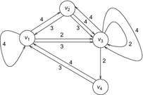
Why haven't we insisted on multiple-edge graphs right away? This is because with the simple cost notion we used in Chapter 1 we can remove multiple edges by keeping only the cheapest ones between the edges for each pair of nodes. The removed edges are superfluous because we are interested in shortest paths. In contrast, we need multiple edges to evidence the need of isotonicity in algebraic costs.
Therefore, the definition of in and out includes graphs with multiple edges on node pairs. Multiple-edge problem graphs have a distinguished start node s, which we denote with  , or just
  if G is clear from the context. For an alternating sequence of nodes and edges
  , such that for each
  we have
  ,
,  ,
,  , and
, and  , or, shortly
  .
.
An initial path is a path starting at s. Finite paths are required to end at nodes. The length of a finite path p is denoted by  . The concatenation of two paths p, q is denoted by pq, where we require p to be finite and end at the initial node of q. The cost of a path is given by the cumulative cost of its edges.
On general cost structures, not all subpaths of an optimal path are necessarily optimal. A path 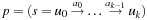 is prefix-optimal if all prefixes of this path
  with
with  form an optimal path. As an example consider the (max/min) cost structure of the problem graph in Fig. 2.20. Path
  and path
  are optimal with cost 2, but only
  is prefix-optimal.
Reachability and optimality problems can be solved with traditional search algorithms. For the reachability problem, for instance, we can use, among others, depth-first search. For the optimality problem, on the other hand, only Dijkstra's algorithm or A* are appropriate. They are traditionally defined over a simple instance of our cost algebra, namely the optimization cost algebra  . Thus, we need to generalize the results that ensure the optimality of the search algorithms; that is, the fact that they correctly solve the optimality problem.
The design of cost-algebraic algorithms depends on a different notion for the principle of optimality, which intuitively means that the optimality problem can be decomposed.
Definition 2.4
(Principle of Optimality) The principle of optimality requires 
 , where s is the start node in a given problem graph G.
Lemma 2.5
Any cost algebra  satisfies the principle of optimality.
Proof
We have The first step is by definition and the second step by the distributivity of ×. The third step is by isotonicity, since
  for all a implies
  , and the last step is by definition.
Next we adapt the notions of admissibility and consistency of heuristic functions.
Definition 2.5
(Cost-Algebraic Heuristics) A heuristic function h with  for each goal node
  is
is
• admissible, if for all  we have
  ;
;
• consistent, if for each  ,
,  with
with  we have
  .
.
We can generalize the fact that consistency implies admissibility.
Lemma 2.6
(Consistency Implies Admissibility) If h is consistent, then it is admissible.
Proof
We have  for some solution path
  ,
,  , and
, and 
We can extend the approach to more than one optimization criterion; for example, for the prioritized Cartesian product of two cost algebras  and
and 

 , which is defined by
  is a tuple
  , where
  ,
,  , and
, and  . Cartesian products that prioritize one criteria among the others have the problem to deliver nonisotone algebras in general (see Exercises).
Lemma 2.7
(Cartesian Product Cost Algebra) If  ,
,  are cost algebras and
  is strictly isotone then
  is a cost algebra.
Proof
The only nontrivial part is isotonicity. If we have  then there are two cases. First,
  , in which case (by strict isotonicity) we have
  and
and  , which clearly implies
  and
and  .
.
The second case is  and
and  . This trivially implies
  and
and  and, by isotonicity,
  and
and  . Clearly, we have
  and
and  .
.
Similarly, we can show that if  and
and  are strictly isotone then
  is strictly isotone (see Exercises).
2.3.2. Multiobjective Search
Many realistic optimization problems, particularly those in design, require the simultaneous optimization of more than one objective function. As an example for bridge construction, a good design is characterized by low total mass and high stiffness. A good aircraft design requires simultaneous optimization of fuel efficiency, payload, and weight. A good sunroof design in a car minimizes the noise the driver hears and maximizes the ventilation. With cost algebras we could preserve the work on certain cross-products of criteria. In the multiobjective case we have now arrived at vectors and partial orders.
A multiobjective search is an extension to traditional search algorithms, where edge costs are vectors. It generalizes a cost-algebraic search and is applicable in various domains where one has several conflicting objectives with solutions that are optimal for the one but not the others. More formally, multiobjective search can be stated as follows. We are given a weighted problem graph G with n nodes, e edges, and cost function  . We additionally have a start node s and a set of goal nodes T. The goal is to find the set of nondominated solution paths in G from s to T, where dominance is given in the form of the following partial order relation
  : For all
  we have
  if
if  for all
  . A vector
  is dominated in set
  if there is a
  in A with
  . The aim is to find solutions that are nondominated such that there exists no other feasible solution that will yield an improvement in one objective without causing a degradation in at least one other objective. Figure 2.21 provides a graph with six nodes and cost vector pairs associated with each edge.
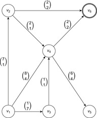
In difference to the cost-algebraic search, relation  is not a total order. Hence, it is not always possible to rank two elements in
  with respect to
  . For example, take
  and
and  . Heuristics
  estimate the accumulated cost vectors of paths to set T. Heuristic h is admissible if for all nondominated solution paths,
 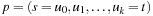 ,
,  , and for all prefix paths
  we have
  .
.
Since most approaches illustrated earlier do not easily translate into a multiobjective search, solving them remains being a challenge.
2.4. Summary
In this chapter, we discussed several search algorithms and their properties. Some search algorithms find a path from the given start state to any of the given goal states; others find paths from the given start state to all other states; and even others find paths from all states to all other states. Desirable properties of search algorithms include their correctness (they find a path if and only if one exists), optimality (they find a shortest path), a small runtime, and small memory consumption. In some cases, the correctness or optimality of a search algorithm is only guaranteed on special kinds of graphs, such as unit or nonnegative cost graphs, or where the goal distances of all states are nonnegative. We are often forced to make trade-offs between the different properties, for example, find suboptimal paths because the runtime or memory consumption would otherwise be too large.
We discussed that most search algorithms perform dynamic programming as an underlying technique. Dynamic programming is a general problem-solving technique that assembles the solutions of complex problems from solutions to simpler problems, which are calculated once and reused several times. Dynamic programming works over the entire state space as a whole, in contrast to heuristic search algorithms, which focus on finding only the optimal path for a single current state and prune everything else for efficiency.
On the other hand, most heuristic search algorithms apply dynamic programming updates and traverse the state space in the same way. They build a tree from the given start state to the goal state, maintaining an estimate of the start distances of all states in the search tree. The interior nodes are in the Closed list and the leaf nodes are in the Open list. They repeatedly pick a leaf of the search tree and expand it; that is, generate its successors in the state space and then add them as its children in the search tree. (They differ in which leaves they pick.) They can find a path from the start state to any of the given goal states if they stop when they are about to expand a goal state and return the only path from the root of the search tree to this goal state. They can find paths from the start state to all other states if they stop only when they have expanded all leaf nodes of the search tree. We distinguished uninformed and informed search algorithms. Uninformed search algorithms exploit no knowledge in addition to the graphs they search. We discussed depth-first search, breadth-first search, Dijkstra's algorithm, the Bellman-Ford algorithm, and the Floyd-Warshall algorithm in this context.
Informed (or synonymously, heuristic) search algorithms exploit estimates of the goal distances of the nodes (heuristic values) to be more efficient than uninformed search algorithms. We discussed A* in this context. We discussed the properties of A* in detail since we discuss many variants of it in later chapters. A* with consistent heuristics has many desirable properties:
• A* can find a shortest path even though it expands every state at most once. It does not need to reexpand states that it has expanded already.
• A* is at least as efficient as every other search algorithm in the sense that every search algorithm (that has the same heuristic values available as A*) needs to expand at least the states that A* expands (modulo tie-breaking; that is, possibly except for some states of which the f-values are equal to the length of the shortest path).
• A* with any given heuristic values cannot expand more states than A* with heuristic values that are dominated by the given heuristic values (again modulo tie-breaking).
Many of these properties followed from the properties of Dijkstra's algorithm, since A* for a given search problem and heuristic values behave identically to Dijkstra's algorithm on a search problem that can be derived from the given search problem by changing the edge costs to incorporate the heuristic values.
Table 2.5 summarizes the uninformed and informed search algorithms, namely how to implement their Open and Closed lists, whether they can exploit heuristic values, which values their edge costs can take on, whether they find shortest paths, and whether or not they can reexpand states that they have expanded already. (The figures that describe their pseudo code are given in parentheses.) Most search algorithms build either on depth-first search or on breadth-first search, where depth-first search trades off runtime and optimality for a small memory consumption and breadth-first search does the opposite. Many discussed algorithms relate to breadth-first search: Dijkstra's algorithm is a specialized version of A* in case no heuristic values are available. It is also a specialized and optimized version of the Bellman-Ford algorithm in case all edge costs are nonnegative. Breadth-first search, in turn, is a specialized and optimized version of Dijkstra's algorithm in case all edge costs are uniform. Finally, we discussed algebraic extension to the operator costs and generalizations for search problems of which the edge costs are vectors of numbers (e.g., the cost and time required for executing an action), explaining why dynamic programming often cannot solve them as efficiently as graphs of which the edge costs are numbers because they often need to maintain many paths from the start state to states in the search tree.
| Algorithm | Open | Closed | Heur | Weight | Optimal | Reopen |
|---|---|---|---|---|---|---|
| DFS (Algorithm 2.1 and Algorithm 2.3) | stack | set | – | unit | – | – |
| BFS (Algorithm 2.1 and Algorithm 2.3) | queue | set | – | unit | √ | – |
| Dijkstra (Algorithm 2.1 and Algorithm 2.4) | pq | set | – | √ | – | |
| Bellm.-Ford (Algorithm 2.7 and Algorithm 2.8) | queue | set | – | √ | √ | |
| A (Algorithm 2.1 and Algorithm 2.5) | pq | set | – | √ | √ | |
| Node-Sel. A (Algorithm 2.1 and Algorithm 2.6) | set | set | – | √ | √ | |
| Floyd-Warshall (2.9) | row | matrix | – | √ | – | |
| A*, cons. (Algorithm 2.1 and Algorithm 2.4) | pq | set | √ | √ | – | |
| A*, admis. (Algorithm 2.1 and Algorithm 2.5) | pq | set | √ | √ | √ | |
| Policy-Iteration (2.11) | set | set | – | prob. | √ | √ |
| Value-Iteration (2.12) | set | set | √ | prob. | ϵ | √ |
2.5. Exercises
2.1 The Missionary and Cannibals (or Hobbits and Orcs) problem is defined as follows (see Fig. 2.22). At one side of a river there are three missionaries and three cannibals. They have a boat that can transport at most two persons. The goal for all persons is to cross the river. At no time should the number of cannibals exceed the number of missionaries for obvious reasons.
1. Draw the problem graph and provide its adjacency list representation.
2. Solve the problem via DFS and BFS by annotating the graph with numbers.
3. Consider a heuristic function that counts the number of people on the other side of the river. Do you observe an inconsistency?
4. Consider a compressed problem graph with actions that correspond to two successive river crossings. Use the same heuristic function as before. Is it consistent?
1. A man, a fox, a goose, and some corn are together on one side of the river. The boat can carry the man and one other subject. The goal is to move them on the other side. Neither the goose and the corn, nor the fox and the goose can be left alone.
2. Four couples have to cross a river that has one island. The boat carries only two persons and because partners are jealous, no person can be left alone with another single of a different sex.
2.3 The Knight's Tour problem asks for a square disjoint on a  -size chess board; that is, for a path that covers the entire board and visits each square only once.
1. Show that there is no Knight's Tour on a  board.
2. A Knight's Tour on the  board is as follows:
| 1 | 18 | 13 | 22 | 7 |
| 12 | 23 | 8 | 19 | 14 |
| 17 | 2 | 21 | 6 | 9 |
| 24 | 11 | 4 | 15 | 20 |
| 3 | 16 | 25 | 10 | 5 |
Compute a Knight's Tour starting top-left and ending two squares right of the bottom-left corner for boards sized  ,
,  ,
,  , and
, and  .
.
3. A Knight's Tour on a square board of size  with a square of size
  omitted in the bottom-right corner, which starts top-right, and ends two squares right of the bottom-left corner looks as follows:
| 32 | 3 | 14 | 9 | 26 | 1 |
| 13 | 24 | 33 | 2 | 15 | 10 |
| 4 | 31 | 12 | 25 | 8 | 27 |
| 23 | 20 | 29 | 34 | 11 | 16 |
| 30 | 5 | 18 | 21 | 28 | 7 |
| 19 | 22 | 35 | 6 | 17 |
Construct similar tours for the boards  with a subsquare of size
  omitted,
  with a subsquare of size
  omitted, and
  with a subsquare of size
  omitted.
4. Use the previous results to devise a Knight's Tour strategy for covering any  board,
  , starting top-right. You will have to reflect some of the subtour patterns along the axes and diagonals.
2.4 Consider the Multiple Sequence Alignment problem between ACGTACGACGT and ATGTCGTACACGT. Take the same cost function as in Exercise 1.16.
1. Fill the dynamic programming table. How best to traverse it?
2. Display the extracted solution path, after the table has been filled.
2.5 Consider the graph in Figure 2.23. Denote the order of expanded nodes (and their f-values) as generated by DFS and BFS, as well as by A* and a greedy best-first search with the Euclidean distance estimate. To resolve ties, nodes should be inserted into the according data structures with respect to their alphabetic order.

2.6 Let graph  be a weighted graph, and T be a set of goal nodes. Suppose that for each node
  reachable from the source we have
  . Show that the graph contains no negative cycle that is reachable from the source.
2.7 Consider the algorithm of Bellman and Ford (on a connected graph).
1. Show that the number of reopenings of a node can be bounded by the length (number of edges) L of an optimal solution path, so that the complexity of the algorithm is  .
.
2. Assign an order  to the nodes of the input graph and partition E in
  and
and  , where
  and
and  .
.  is acyclic with topological order
  and
and  is acyclic with topological order
  . Now relax all edges in
  leaving
  for all
  in
in  and all edges in
  leaving
  for all
  in
in  . Show that
  passes suffice.
3. Another refinement is that if  ,
,  are the strongly connected components of G. (Recall that a and b are in the same strongly connected components if a can reach b and b can reach a.) Show that the algorithm now runs in time
  .
.
2.8 Knapsack has the following inputs: weights  , utilities
  , and weight limit W. Putting an item i into the knapsack increases the weight of the knapsack by
  and gives an additional utility of
  . The optimization problem is to maximize the utility in the set of all possible packings, while respecting the weight limit. The corresponding decision problem additionally takes a bound U for the utility as the input.
1. Show that Knapsack can be solved in time  by dynamic programming.
2. Extend the algorithm to compute the optimal packing.
2.9 The product C of two matrices A and B having respective sizes  and
and  is defined by
  , for
, for  and
and  . Devise a dynamic programming algorithm to compute the matrix product of
  (of sizes
  ,
,  ,
,  ,
,  ,
,  , and
, and  ) with a minimal number of multiplications.
1. Determine the number of multiplications needed to compute  and
and  .
.
2. Find an arrangement of brackets with the least number of multiplications.
3. How many options are there to place brackets?
2.10 Prove the correctness of cost-algebraic search variants.
1. Show that the cost-algebraic version of Dijkstra's algorithm solves the optimality problem on multiple-edge graphs.
2. simple Show that cost-algebraic A* for consistent estimates solves the optimality problem on multiple-edge graphs.
4. Infer that cost-algebraic A* with reopening solves the optimality problem for admissible estimates on multiple-edge graphs.
2.11 Prove that if  and
and  are both strictly isotone, then
  is strictly isotone.
2.13 Solve the following Wumpus World problem via value iteration and policy iteration: a  Gridworld with a hole at
  , and two goals at
  and
and  . The agent starts at
  ; the rewards are: 1, for arriving at
  , and −1, for arriving at
  . Transition probabilities for the four possible move directions are as follows. With probability
  the move is successful; with probability of
  (each) the move direction misplaced at right angles. If a wall is encountered, the agent stays at its position. As discount value
  take 24/25. For both cases restrict the number of iterations to 50.
1. Display the stochastic transition system, with states and transition probabilities.
2. Provide the reward cost table.
2.14 Show that the ϵ-greedy policies with respect to  are an improvement over every policy with
  .
.
2.6. Bibliographic Notes
Shortest path search is a classic topic in the field of combinatorial optimization. The algorithm of Dijkstra (1959) to find shortest paths in graphs with nonnegative edge weights is one of the most important algorithms in computer science. Sound introductions to shortest path search are given by Tarjan (1983) and Mehlhorn (1984). The linear-time shortest path algorithm for acyclic graphs can be found in Lawler (1976).
Using lower bound to prune search goes back to the late 1950s, where branch-and-bound search was proposed. The first use of distance goal estimates to guide state space search is probably due to Doran and Michie (1966) in a program called GraphTraverser. Original A* search as proposed by Hart, Nilsson, and Raphael (1968) refers to Dijkstra's algorithm, but in most AI textbooks the link to standard graph theory has vanished. The reweighting transformation is found in Cormen, Leiserson, and Rivest (1990) in the context of the All Pairs Shortest Paths problem of Johnson (1977). It makes it abundantly clear that heuristics do not change the branching factor of a space, but affect the relative depth of the goal, an issue stressed while predicting the search efforts of IDA*. The general problem of finding the shortest path in a graph containing cycles of negative length is NP-hard (Garey and Johnson, 1979).
Bellman (1958) and Ford and Fulkerson (1962) discovered the algorithm for shortest path search in negative graphs independently. A nondeterministic version is discussed by Ahuja, Magnanti, and Orlin (1989). Gabow and Tarjan (1989) showed that if C is the weight of the largest edge the algorithm of Bellman and Ford can been improved to  . To alleviate the problem of exponentially many node expansions in A*, Martelli (1977) suggested a variation of the Bellman-Ford algorithm, where the relaxation is performed for the entire set of expanded nodes each time a new node is considered. His algorithm has been slightly improved by Bagchi and Mahanti (1983). The heuristic search version of the Bellman-Ford algorithm were entitled C, ProbA, and ProbC (Bagchi and Mahanti, 1985). Mero (1984) has analyzed heuristic search with a modifiable estimate in an algorithm B′ that extends the B algorithm of Martelli (1977). A taxonomy of shortest path search has been given by Deo and Pang (1984) and a general framework that includes heuristic search has been presented by Pijls and Kolen (1992). Sturtevant, Zhang, Holte, and Schaeffer (2008) have analyzed inconsistent heuristics for A* search, and propose a new algorithm that introduces a delay list for a better trade-off.
The technique of dynamic programming has been introduced by Bellman (1958). One of the most important applications of this principle in computer science is probably the parsing of context-free languages (Hopcroft and Ullman, 1979; Younger, 1967). Computing edit-distances with dynamic programming is a result that goes back to mathematicians like Ulam and Knuth. In computational biology, the work of Needleman and Wunsch (1981) is considered as the first publication that applies dynamic programming to compute the similarity of two strings. A neat application also used for compiling this textbook is the optimal line break algorithm of Knuth and Plass (1981). A good introduction to the subject of dynamic programming is found in the textbook of Cormen et al. (1990). The lattice edge representation for multiple sequence alignment has been adopted in the program MSA by Gupta, Kececioglu, and Schaffer (1996).
The term best-first search appears in AI literature in two different meanings. Pearl (1985) uses this term to define a general search algorithm that includes A* as a special case. Others use it to describe an algorithm that always expands the node estimated closest to the goal. Russell and Norvig (2003) coined the term greedy best-first search to avoid confusion. In our notation an algorithm is optimal if it computes a shortest solution path. We chose an optimal instead of an admissible algorithm as done by Pearl (1985). Optimality in our notation does not mean optimal efficiency. The optimality efficiency argument on the number of node expansions in A* with consistent heuristics has been given by Dechter and Pearl (1983). Common misconceptions of heuristic search have been highlighted by Holte (2009).
The cost formalism extends the one of Sobrinho (2002) with an additional set, to where the heuristic function is mapped. The problem of Cartesian products and power constructions as defined for semirings by Bistarelli, Montanari, and Rossi (1997) is that they provide partial orders. Observations on multiobjective A* have been provided by Mandow and de-la Cruz (2010a,b). Multiobjective IDA* has been considered by Coego, Mandow, and de-la Cruz (2009). Speed-up techniques for a Dijkstra-like search have been studied by Berger, Grimmer, and Müller-Hannemann (2010). Advances in multiobjective search also include work on minimum spanning trees by Galand, Perny, and Spanjaard (2010) as well as Knapsack problems by Delort and Spanjaard (2010).
..................Content has been hidden....................
You can't read the all page of ebook, please click here login for view all page.