
Chapter 13. Constraint Search
This chapter gives a general introduction to constraint satisfaction. It discusses traditional constraint satisfaction problems, temporal constraint networks, and critical path scheduling, and turns to different NP-hard optimization problems. It also discusses recent results on searching backbones and backdoors as well as path and soft constraints
Keywords: consistency, arc consistency, bounds consistency, path consistency, backtracking, backjumping, backmarking, Boolean satisfiability, number partition, bin packing, rectangle packing, vertex cover, independent set, clique, graph partition, temporal constraint network, simple temporal network, PERT scheduling, formula progression, automata encoding, soft constraints, preference constraints, path constraints.
Constraint technology has evolved into one of the most effective search options, which is understandable because its declarative formulation makes it easy to use. The technology is open and extensible, because it differentiates among branching, propagation, and search. Constraint search has been integrated (e.g., in the form of a library) to many existing programming languages and is effective in many practical applications, especially in time tabling, logistics, and scheduling domains.
A search constraint is a restriction on the set of possible solutions to a search problem. For goal constraints (the standard setting in state space search), we specify goal states, and these incorporate constraints on the goal. In this case, constraints refer to the end of solution paths, denoting the restriction on the set of possible terminal states. For path constraints, constraints refer to the path as a whole. They are expressed in temporal logic, a common formalism for the specification of desired properties of software systems. Examples are conditions that have to be satisfied always, or achieved at least sometimes during the execution of a solution path.
In constraint modeling we have to decide about variables, their domains, and constraints. There are many different options to encode the same problem, and a good encoding may be essential for an efficient solution process.
Constraints can be of very different kinds; special cases are binary and Boolean constraints. The former ones include at most two constraint variables in each constraint to feature efficient propagation rules, and the latter ones refer to exactly two possible assignments (true and false) to the constraint variables and are known as satisfiability problems.
We further distinguish between hard constraints that have to be satisfied, and soft constraints, the satisfaction of which is preferred but not mandatory. The computational challenge with soft constraints is that they can be contradicting. In such cases, we say that the problem is oversubscribed. We consider soft constraints to be evaluated in a linear objective function with coefficients measuring their desirability.
Constraints express incomplete information such as properties and relations over unknown state variables. Search is needed to restrict the set of possible value assignments. The search process that assigns values to variables is called labeling. Any assignment corresponds to imposing a constraint on the chosen variable. Alternatively, general branching rules that introduce additional constraints may be used to split the search space.
The process to tighten and extend the constraint set is called constraint propagation. In constraint search, labeling and constraint propagation are interleaved. As the most important propagation techniques we exploit arc consistency and path consistency. Specialized consistency rules further enhance the propagation effectiveness. As an example, we explain insights to the inference based on the all-different constraint that requires all variable assignments to be mutually different.
Search heuristics determine an order on how to traverse the search tree. They can be used either to enhance pruning or to improve success rates, for example, by selecting the more promising nodes for a feasible solution. Different from the observation in previous chapters, for constraint search, diverse search paths turn out to be essential. Consequently, as one heuristic search option, we control the search by the number of discrepancies to the standard successor generation module.
Most of the text is devoted to strategies for solving constraint satisfaction problems, asking for satisfying assignments to a set of finite-domain variables. We also address the more general setting of solving constraint optimization problems, which asks for an optimal value assignment with respect to an additionally given objective function. For example, problems with soft constraints are modeled as a constraint optimization problem by introducing additional state variables that fine the violation of preference constraints. We will see how search heuristics in the form of lower bounds can be included into the constraint optimization, and how more general search heuristics apply.
In later parts of the chapter, we subject the search to solving some well-known NP-hard problems with specialized constraint solvers. We will consider instances of SAT, Number Partition, Bin Packing, and Rectangle Packing, as well as graph problems like Graph Partition and Vertex Cover. We present heuristic estimates and further search refinements to enhance the search for (optimal) solutions.
Temporal constraints are ones that restrict the set of possible time points; for example, to wake up between 7 a.m and 8 a.m. For this case variable domains are infinite. We introduce two algorithmic approaches that can deal with temporal constraints.
13.1. Constraint Satisfaction
Constraint satisfaction is a technology for modeling and solving combinatorial problems. Its main parts are domain filtering and local consistency rules together with refined search techniques to traverse the resulting state space. Constraint satisfaction relies on a declarative problem description that consists of a set of variables together with their respective domains. Each domain itself is composed of a set of possible values. Constraints restrict the set of possible combinations of the variables.
Constraints are often expressed in the form of arithmetic (in)equalities over a set of unknown variables; for example, the unary integer constraints X ≥ 0 and X ≤ 9 denote that the value X consists of one digit. Combining a set of constraints can exploit information and yield a set of new constraints. Arithmetic linear constraints, such as X + Y = 7 and X − Y = 5, can be simplified to the constraints: X = 6 and Y = 1. In constraint solving practice, elementary calculus is often not sufficient to determine the set of feasible solutions. In fact, most constraint satisfaction domains we consider are NP-hard.
Definition 13.1
(CSP, Constraint, Solution) A constraint satisfaction problem (CSP) consists of a finite set of variables  of finite domains
  , and a finite set of constraints, where a constraint is a(n arbitrary) relation over the set of variables. Constraints can be extensional in the form of a set of compatible tuples or intentional in the form of a formula. A solution to a CSP is a complete assignment of values to variables satisfying all the constraints.
For the sake of simplicity this definition rules out continuous variables. Examples for extending this class are considered later in this chapter in the form of temporal constraints.
A binary constraint is a constraint involving only two variables. A binary CSP is a CSP with only binary constraints. Unary constraints can be compiled into binary ones, for example, by adding constraint variables with only assignment 0.
Any CSP is convertible to a binary CSP via its dual encoding, where the roles of variables and constraints are exchanged. The constraint variables are encapsulated, meaning one has assigned a domain that is a Cartesian product of the domains of individual variables. The valuation of original variables can to be extracted from the valuation of encapsulated variables. As an example, take the original (non-binary) CSP: X + Y = Z, X < Y, with  ,
,  , and
, and  . The equivalent binary CSP consists of the two encapsulated variables
  and
and  together with their domains
  and
and  . The binary constraints between V and W require that the components that refer to the same original variables match; for example, the first component in V (namely X) is equal to the first component in W and the second component in V(namely Y) is equal to the second component in W.
One example is the Eight Queens problem (see Fig. 13.1). The task is to place eight queens on a chess board, but with at most one queen in the same row, column, or diagonal. If variable Vi denotes the column of the queen in row i,  , we have that
  . An assignment to one variable will restrict the set of possible assignments to other ones. The constraints that induce no conflict are Vi ≠ Vj (vertical threat) and
  (diagonal threat) for all 1 ≤ i ≠ j ≤ 8. (Horizontal threats are already taken care of in the constraint model.)

Such a problem formulation calls for an efficient search algorithm to find a feasible variable assignment representing valid placements of the queens on the board. A naive strategy considers all 88 possible assignments, which can easily be reduced to 8!. A refined approach maintains a vector for a partial assignment in a vector, which grows with increasing depth and shrinks with each backtrack. To limit the branching during the search, we additionally maintain a global data structure to mark all places that are in conflict with the current assignment.
A Sudoku (see Fig. 13.2) is a puzzle with rising popularity in the United States, but with a longer tradition in Asia and Europe. The rules are simple: fill all empty squares with numbers from  such that in each column, in each row, and in each 3 × 3 block, all numbers from 1 to 9 are selected exactly once. If variable Vi,j with
  denotes the number assigned to cell (i, j), where
  , as constraints we have
•  for all
  ,
,  (vertical constraints)
•  for all
  ,
,  (horizontal constraints)
•  for all
  ,
,  and
and  (subsquare constraints)
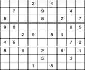 |
| Figure 13.2 |
As another typical CSP example, we consider a Cryptarithm (a.k.a crypto-arithmetic puzzle or alphametic), in which we have to assign numbers to each individual variable, so that the equation SEND + MORE = MONEY becomes true. The set of variables is {S, E, N, D, M, O, R, Y}. Each variable is an integer from 0 to 9, and leading characters and S and M cannot be assigned 0. The problem is to assign pairwise different values to the variables. It is not difficult to check that the (unique) solution to the problem is given by the assignments [S, E, N, D, M, O, R, Y] = [9, 5, 6, 7, 1, 0, 8, 2] (vector notation).
Since we only consider problems with decimal digits, there are at most 10! different assignments of the digits to variables. So a Cryptarithm is a finite-state space problem, but generalizations to bases other than decimals are provably hard (NP-complete).
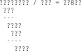
Another famous CSP problem is the Lonely Eight problem. The task is to determine all wild cards in the division that is shown in Figure 13.3. For a human using basic calculus and exclusions it is not difficult to obtain the only solution  . However, since no specialized constraints can be used, CSP solvers are often confronted with considerable work.
13.2. Consistency
Consistency is an inference mechanism to rule out certain variable assignments, which in turn enhances the search. The simplest consistency check tests a current assignment against the set of constraints. Such a simple consistency algorithm for a set of assigned variables and a set of constraints is provided in Algorithm 13.1. We use Variables(c) to denote the set of variables that are mentioned in the constraint c, and Satisfied(c, L) to denote if the constraint c is satisfied by the current label set L(assignment of values to variables).
In the following we introduce more powerful inference methods like arc consistency and path consistency, and discuss specialized consistency techniques like the all-different constraint.
13.2.1. Arc Consistency
Arc consistency is one of the most powerful propagation techniques for binary constraints. For every value of a variable in the constraint we search for a supporting value to be assigned to the other variable. If there is none, the value can safely be eliminated. Otherwise, the constraint is arc consistent.
Definition 13.2
(Arc Consistency) The pair (X, Y) of constraint variables is arc consistent if for each value  there exists a value
  such that the assignments X = x and Y = y satisfy all binary constraints between X and Y. A CSP is arc consistent if all variable pairs are arc consistent.
Consider a simple CSP with the variables A and B subject to their respective domains  and
and  , as well as the binary constraint A < B. We see that value 1 can be safely removed from DB based on constraint and the restriction we have on A.

In general, constraints are used actively to remove inconsistencies from the problem. An inconsistency arises if we arrive at a value that cannot be contained in any solution. To abstract from different inference mechanisms we assume a procedure Revise, to be attached to each constraint, which governs the propagation of the domain restrictions.
AC-3 and AC-8
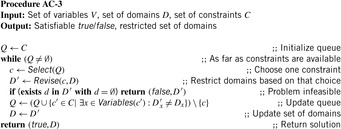
Algorithm AC-3 is one option to organize and perform constraint reasoning for arc consistency. The input of the algorithm are the set of variables V, the set of domains D, and the set of constraints C.
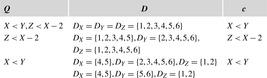
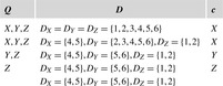
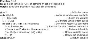
In the algorithm, a queue of constraints is frequently revised. Each time, when the domain of a variable changes, all constraints over this variable are enqueued. The pseudo code of the approach is shown in Algorithm 13.2. As a simple example, take the following CSP with the three variables  , subject to the binary constraints X < Y and Z < X − 2. As X < Y, we have
  ,
,  , and
, and  . Since Z < X − 2, we infer that
  ,
,  , and
, and  . Now we take constraint X < Y again to find the arc consistent set
  ,
,  , and
, and  . Snapshots of the algorithms after selecting variable c are provided in Figure 13.4.
 |
| Figure 13.4 |
An alternative to AC-3 is to use a queue of variables instead of a queue of constraints. The modified algorithm is referred to as AC-8. It assumes that a user will specify, for each constraint, when constraint revision should be executed. The pseudo code of the approach is shown in Algorithm 13.3 and a step-by-step example is given in Figure 13.5.
13.2.2. Bounds Consistency
Arc consistency works well in binary CSPs. However, if we are confronted with constraints that involve more than two variables (e.g., X = Y + Z), the application of arc consistency is limited. Unfortunately, hyperarc consistency techniques are involved, and similar to the complexity of Set Covering and Graph Coloring-NP-hard for n ≥ 3. The problem is that we must determine which values of the variables are legitimate and which is a nontrivial problem.
The trick is to use an approximation of the set of possible assignments in the form of an interval. A domain range  denotes the set of integers
  with minD = a and maxD = b.
For bounds consistency we only look at arithmetic CSPs that range over finite-domain variables for which all constraints are arithmetic expressions. A primitive constraint is bounds consistent if for each variable X that is in the constraint there is an assignment for all other variables (in their domain range) that is compatible with setting X to minD and X to maxD. An arithmetic CSP is bounds consistent if each primitive constraint is bounds consistent.
Consider the constraint X = Y + Z and rewrite it as X = Y + Z, Y = X − Z, and Z = X − Y. Reasoning about minimum and maximum values on the right side, we establish the following six necessary conditions:  ,
,  ,
,  ,
,  ,
,  , and
, and  . For example, the domains
  ,
,  , and
, and  are refined to
  ,
,  , and
, and  without missing any solution.
13.2.3. *Path Consistency
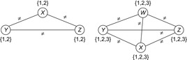
The good news about arc consistency is that it is fast in practice. The bad news is that arc consistency does not detect all inconsistencies. As a simple example consider the CSP shown in Figure 13.6 (left) with the three variables X, Y, Z with  subject to X ≠ Y, Y ≠ Z, and X ≠ Z. The CSP is arc consistent but not solvable. Therefore, we introduce a stronger form of consistency.
 |
| Figure 13.6 |
Definition 13.3
(Path Consistency) A path  is path consistent if, for all x in the domain of V0, and for all y in the domain of Vm satisfying all binary constraints on V0 and Vm, there exists an assignment to
  , s.t. all binary constraints between Vi and Vi+1 for
  are satisfied.
A CSP is path consistent, if every path is consistent.
This definition is long but not difficult to decipher. On top of binary constraints between two variables, path consistency certifies binary consistency between the variables on a path. It is not difficult to see that path consistency implies arc consistency. An example to show that path consistency is still incomplete is provided in Figure 13.6 (right).
For restricting the computational efforts, it is sufficient to explore paths of length two only (see Exercises). To come up with a path consistency algorithm, we consider the following example, consisting of the three variables A, B, C with DA = DB = DC = {1, 2, 3}, subject to B > 1, A < C, A = B, and B > C − 2. Each constraint can be expressed in a (Boolean) matrix, denoting whether a variable combination is possible or not: Let Ri,j be the matrix entry for the constraint between variable i and j; Rk,k models the domain of k. Then consistency on the path (i, k, j) can be recursively determined by applying the equation
 The concatenations correspond to Boolean matrix multiplications, such as the scalar product of the rows and columns in the matrix. The final conjunction is element-by-element.
For the example  , we establish the following equation:
 We observe that path consistency restricts the set of possible instantiations in the constraint.
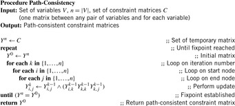
For a path-consistent CSP, we have to repeat the earlier revisions of paths. The pseudo code is shown in Algorithm 13.4. It is a straightforward extension to the All-Pairs Shortest Paths algorithm of Floyd and Warshall (see Ch. 2). Mathematically spoken, it is the same algorithm applied to a different semiring, where minimization is substituted by conjunction and addition is substituted by multiplication.
13.2.4. Specialized Consistency
As path consistency is comparably slow with respect to arc consistency, it is not always the best solution for overall CSP solving. In some cases specialized constraints (together with effective propagation rules) are often more effective.
One important specialized constraint is the all-different constraint (AD) that we already came across in the Sudoku and Cryptarithm domains at the beginning of this chapter.
Definition 13.4
(All-Different Constraint) The all-different constraint covers a set of binary inequality constraints among all variables X1 ≠ X2, X1 ≠ X3, …, Xk−1 ≠ Xk:
Propagating the all-different constraint, we achieve strong pruning. Its efficient implementation is based on matching bipartite graphs, where the set of nodes V is partitioned into two disjoint sets V′ and V′′: for each edge its source and target nodes are contained in a different set, and a matching is a node-disjoint selection of edges.
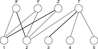
The assignment graph for the all-different constraint consists of two sets. On one hand, we have the variables, and, on the other hand, we have the values that are in the domain of at least one of the variables. Any assignment to the variables that satisfies the all-different constraint is a maximum matching. The running time for solving bipartite matching problems in graph G = (V, E) is  (using maximum flow algorithms). An example for the propagation of the all-different constraint is provided in Figure 13.7.
13.3. Search Strategies
As with path consistency, even strong propagation techniques are often incomplete. Search is needed for resolving the set of remaining uncertainties for the current variable assignments.
The most important way to span a search tree is labeling, which assigns different values to variables. In a more general view, the search for solving constraint satisfaction problems resolves disjunctions. For example, an assignment not only assigns variables on one branch but also denotes that this value is no longer available on other branches of the search tree.
This observation leads to very different branching rules to generate a CSP search tree. They define the shape of the search tree. As an example, we can produce a binary search tree, by setting  for one particular value x and branch on only these two constraints. Another important branching rule is domain splitting, which also generates a binary search tree. An example is to split the search tree according to the disjunction
  . The next option is disjunctions on the variable ordering, such as
  .
.
Walking along this line, we see that each search tree node can be viewed as a set of constraints, indicating which knowledge on the set of variables is currently known for solving the problem. For example, assigning a value x to a variable X for generating a current search tree node u adds the constraint X = x to the constraint set of the predecessor node parent(u).
In the following we concentrate on labeling and on the selection of the variable to be labeled next. One often applied search heuristic is first-fail. It prefers the variable, the instantiation of which will lead to a failure with the highest probability. The intuition behind the strategy is to work on the simpler problems first. A consequent rule for this policy is to test variables with the smallest domain first. Alternatively, we may select most constrained variables first.
For value selection, the succeed-first principle has shown good performance. It prefers the values that might belong to the solution with the highest probability. Value selection criteria define the order of branches to be explored and are often problem-dependent.
13.3.1. Backtracking
The labeling process is combined with consistency techniques that prune the search space. For each search tree node we propagate constraints to make the problem locally consistent, which in turn reduces the options for labeling. The labeling procedure will backtrack upon failure, and continue with a search tree node that has not yet resolved completely.
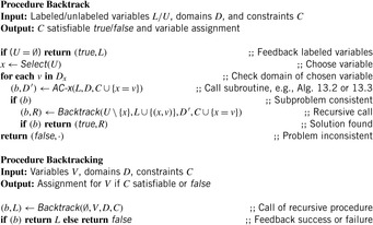
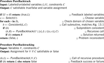
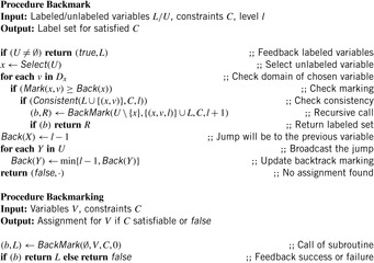
The pseudo code for such a backtracking approach is shown in Algorithm 13.5. In the initial call of the recursive subprocedure Backtrack, the variable assignment set V is divided into the set of already labeled variables L and the set of yet unlabeled variables U. If all variables are successfully assigned the problem is solved and the assignment can be returned. As with the consistency algorithm an additional flag is attached to the return value to distinguish between success and failure.
There is a trade-off between the time spent for search and the time spent for propagation. The consistency call matches the parameters of the arc consistency algorithms AC-3 and AC-8. It is not difficult to include more powerful consistency methods like path consistency. On the other hand, more aggressive consistency mechanisms only check if the current assignment leads to no contradiction with the current set of constraints. Such a pure backtracking algorithm is shown in Algorithm 13.6. Other consistency techniques remove incompatible values only from connected but currently unlabeled variables. This technique is called forward checking. Forward checking is cheap. It does not increase the time complexity of pure backtracking, as the checks are only drawn earlier in the search process.
13.3.2. Backjumping
One weakness of the backtrack procedure is that it throws away the reason for the conflict. Suppose that we are given constraint variables A, B, C, D with  and a constraint A > D. Backtracking starts with labeling A = 1, and then tries all the assignments for B and C before finding that A has to be larger than 1. A better option is to jump back to A at the first time D is labeled, since this is the source of the conflict.
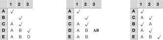
We explain the working of the backjumping algorithm for the example with variables A, B, C, D, E, all of domain {1, 2, 3}, and constraints A ≠ C, A ≠ D, A ≠ E, B ≠ D, E ≠ B, and E ≠ D. The according constraint graph is shown in Figure 13.8. Some snapshots of the backjumping algorithm for this example are provided in Figure 13.9, where the variables are plotted against their possible value assignments following the order of labeling.

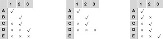 |
| Figure 13.9 Conflict matrix evolution for backjumping in the example of Figure 13.8; matrix entries denote impossible assignment, and check denotes current assignment. Value assignment until first backtrack at E (left). After backtracking from E to the previous level, there is no possible variable assignment (middle). Backjumping to variable B, since this is the source of the conflict, eventually finds a satisfying assignment (right). |
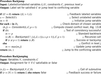
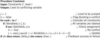
The pseudo code for the backjumping procedure is shown in Algorithm 13.7. The additional parameter for the algorithm is the previous level from which the procedure is invoked. The return value includes the jump level instead of simply denoting success or failure. The values  are the otherwise impossible jump values chosen for success. The implementation is tricky. It invokes a variant of the (simple) consistency check, for which the closest conflicting level is computed, in addition to the test of satisfaction of the constraints. The pseudo code is shown in Algorithm 13.8. Its parameters are the currently label set L, the constraint set C, and the backjump level l. The implementation of Algorithm 13.8 is not much different from Algorithm 13.1 in the sense that it returns a Boolean value, denoting if the consistency check was successful and the level j on which the conflict has been detected. The update of j takes the current label set L into account, which now consists of triples with the third component being the level to which a variable is assigned. This value j then determines the return value in Algorithm 13.7 and the level m for the next backjump.
The reassignment of variable C that is in between B and D is actually not needed. This brings us to the next search strategy.
13.3.3. Dynamic Backtracking
A refinement to backjumping is dynamic backtracking. It handles the problem of losing the in-between assignments when jumping back. Dynamic backtracking remembers the source of the conflict, monitors the source of the conflict, and changes the order of variables.
Consider again the example of Figure 13.8. The iterations shown in Figure 13.10 illustrate how the sources of conflicts are maintained together with the assignments to the variables and how this information eventually allows the change of variable ordering. if we assign A to 1 and B to 2 we need no conflict information. When assigning C to 2 we store variable A at C as the source of a conflict of choosing 1. Setting D to 3 leads to the memorization of conflict with A(value 1) and B(value 2). Now E has no further assignment (left) so that we jump back to D but carry the conflict source AB from variable E to D(middle). This leads to another jump from D to C and a change of order of the variable B and C(right). A final assignment is A to 1, C to 2 (with conflict source A), B to 1 (with conflict source A), D to 2 (with conflict source A), and E to 3 (with conflict sources A and B). In difference to backjumping, vertex C is not reassigned.
 |
| Figure 13.10 Conflict matrix evolution for dynamic backtracking in the example of Figure 13.8; matrix entries denote source of conflict for chosen assignments, check denotes current assignment, bold variables are transposed. |
13.3.4. Backmarking
Another problem for backtracking is redundant work for which unnecessary constraint checks are repeated. For example, consider A, B, C, D with  with the constraints A + 8 < C, B = 5D. Consider the search tree generated by labeling A, B, C, D (in this order). There is much redundant computation in different subtrees when labeling variable C (after setting B = 1, B = 2, …, B = 10). The reason is that the change in B does not influence variable C at all. Therefore, we aim at removing redundant constraint checks.
The proposed solution is to remember previous (either good or no-good) assignments. This so-called backmarking algorithm removes redundant constraint checks by memorizing negative and positive tests. It maintains the values
• Mark(x,v), for the farthest (instantiated) variable x in conflict with the current assignment v (conflict marking).
• Back(x), for the farthest variable to which we backtracked since the last attempt to instantiate x (backtrack marking).
Constraint checks can be omitted for the case Mark(x,v) < Back(x). An illustration is given in Figure 13.11. We detect that the assignment from X to 1 on the left branch on the tree is inconsistent with the assignment of Y to 1, but consistent with all other variables above X. The assignment from X to 1 on the right branch on the tree is still inconsistent with the assignment of Y to 1 and does not need to be checked again.

The pseudo-code implementation is provided in Algorithm 13.9 as an extension to the pure backtracking algorithm. We see that checking if the conflict marking is larger than or equal to the backtrack marking is performed before every consistency check. The algorithm also illustrates how the value Back is updated. The conflict marking is assumed to be stored together with each assignment. Note that as with backjumping (see Alg. 13.8), the consistency procedure is assumed to compute the conflict level together with each call.
The backmarking algorithm is illustrated for the Eight Queens problem of Figure 13.1 in Figure 13.12. The farthest conflict queen (the conflict marking) is denoted on the board, and the backtrack marking is written to the right of the board. The sixth queen cannot be allocated, despite the assignment to the fifth queen, such that all further assignments to the fifth queen are discarded. It is not difficult to observe that backmarking can be combined with backjumping.
 |
| Figure 13.12 |
13.3.5. Search Strategies
In practical application of constraint satisfaction for real-life problems we frequently encounter that search spaces are so huge that they cannot be fully explored.
This immediately suggests heuristics to guide the search process into the direction of an assignment that satisfies the constraints and optimizes the objective function. In constraint satisfaction search heuristics are often encoded to recommend a value for an assignment in a labeling algorithm. This approach often leads to a fairly good solution on the early trials.
Backtracking mainly takes care of the bottom part of the search tree. It repairs later assignments rather than earliest ones. Consequently, backtracking search relies on the fact that search heuristics guide well in the top part of the search tree. As a drawback, backtracking is less reliable in the earlier parts of the search tree. This is due to the fact that, as the search process proceeds, more and more information is available and the number of violations to a search heuristic is small in practice.
Limited Discrepancy Search
Errors in the heuristic values have also been examined in the context of limited discrepancy search (LDS). It can be seen as a modification of depth-first search. On hard combinatorial problems like Number Partition (see later) it outperforms traditional depth-first search.
Given a heuristic estimate, it would be most beneficial to order successors of a node according to their h-value, and then to choose the left one for expansion first. A search discrepancy means to stray from this heuristic preference at some node, and instead examine some other node that was not suggested by the heuristic estimate.
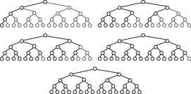
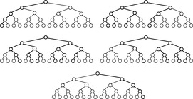
For ease of exposition, we assume binary search trees (i.e., two successors per node expansion). In fact, binary search trees are the only case that has been considered in literature and extensions to multi-ary trees are not obvious. A discrepancy corresponds to a right branch in an ordered tree. LDS performs a series of depth-first searches up to a maximum depth d. In the first iteration, it first looks at the path with no discrepancies, the left-most path, then at all paths that take one right branch, then with two right branches, and so forth. In Figure 13.13 paths with zero (first path), one (next three paths), two (next three paths), and three discrepancies (last path) in a binary tree are shown.
To measure the time complexity of LDS, we count the number of explored leaves.
Theorem 13.1
(Complexity LDS) The number of leaves generated in limited discrepancy search in a complete binary tree of depth d is (d + 2)2d − 1.
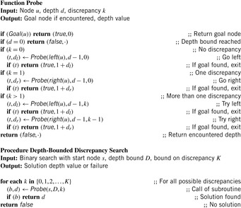
The pseudo code for LDS is provided in Algorithm 13.10. Figure 13.14 visualizes the branches selected (bold lines) in different iterations of linear discrepancy search.
 |
| Figure 13.14 |
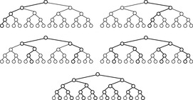
An obvious drawback of this basic scheme is that the i th iteration generates all paths with i discrepancies or less, hence it replicates the work of the previous iteration. In particular, to explore the right-most path in the last iteration, LDS regenerates the entire tree. LDS has been improved later using an upper bound on the maximum depth of the tree. In the i th iteration, it visits the leaf at the depth limit with exactly i discrepancies. The modified pseudo code for improved LDS is shown in Algorithm 13.11. An example is provided in Figure 13.15. This modification saves a factor of (d + 2)/2.
Theorem 13.2
(Complexity-Improved LDS) The number of leaves generated in improved limited discrepancy search in a complete binary tree of depth d is 2d.
Proof
Since each iteration of improved LDS generates those paths with exactly k discrepancies, each leaf is generated exactly once for a total of 2d leaf nodes.
A slightly different strategy, called depth-bounded discrepancy search, biases the search toward discrepancies high up in the search tree by means of an iteratively increasing depth bound. In the i th iteration, depth-bounded discrepancy explores those branches on which discrepancies occur at depth i or less. Algorithm 13.12 shows the pseudo code of depth-bounded discrepancy search. For the sake of simplicity, again we consider the traversal in binary search trees only.
Compared to improved LDS, depth-bounded LDS explores more discrepancies at the top of the search tree (see Fig. 13.16). While improved discrepancy search on a binary tree of depth d explores in its first iteration branches with at most one discrepancy, depth-bounded discrepancy search explores some branches with up to lgd discrepancies.
13.4. NP-Hard Problem Solving
For an NP-complete problem L we require
NP-containment a nondeterministic Turing machine M that recognizes L in polynomial time, and
NP-hardness a polynomial-time transformation f, one for each problem L′ in NP, such that  if and only if
  .
.
The running time of M is defined as the length of the shortest path to a final state. A deterministic Turing machine may simulate all possible computations of M in exponential time. Therefore, NP problems are state space problems with a state space of configurations of M, operators are transitions to successor configurations, the initial state is the start configuration of M, and the goal is defined by its final configuration(s).
NP-completeness makes scaling successful approaches difficult. Nonetheless, hard problems are frequent for search practice and for hundreds of thousands of problem instances that have been classified.
13.4.1. Boolean Satisfiability
Boolean CSPs are CSPs in which all variable domains are Boolean. Hence, the only two assignments that are allowed are true and false. If we are looking at variables of finite domains only, any CSP is convertible to a Boolean CSP, via an encoding of the variable domains. In such an encoding we impose an assignment of the form X = x for each variable X and each value  .
.
Let a literal be a positive or negated Boolean variable, and a clause be a disjunction of literals. We use the truth values true/false and their numerical equivalent 0/1 interchangeably.
Definition 13.5
(Satisfiability Problem) In Satisfiability (SAT) we are given a formula f as a conjunction of clauses over the literals  . The task is to search for an assignment
  for
for  , so that f(a) = true.
By setting x3 to false the example function  is satisfiable.
Theorem 13.3
(Complexity SAT) SAT is NP-complete.
Proof
We only give the proof idea. The containment of SAT in NP is trivial since we can test a nondeterministically chosen assignment in linear time. To show that for all L ∈ NP we have polynomial reduction to SAT, the computation of a nondeterministic Turing machine for L is simulated with (polynomially many) clauses.
Definition 13.6
(k-Satisfiability) In k-SAT the SAT instances consist of clauses of the form
Dealing with clauses of length smaller than k is immediate. For example, by adding the redundant literal  to the second clause, f is converted to 3-SAT notation. Even if k-SAT instances are simpler than general SAT problems, for k ≥ 3 the k-SAT problem is still intractable.
Theorem 13.4
(Complexity k-SAT) k-SAT is NP-hard for k ≥ 3.
Proof
The proof applies a simple local replacement strategy. For each clause C in the original formula,  extra variables are introduced for linking shorter clauses together. For example, satisfiability of
  is equivalent to satisfiability of the 3-SAT formula
  .
.
It is known that 2-SAT is in P. Since  is equivalent to
  and
and  , respectively, we construct a graph Gf with nodes
  and edges that correspond to the induced implications. It is not difficult to see that f is not satisfiable, if and only if Gf has a cycle that contains the same variable, once positive and once negative.
David-Putnam Logmann-Loveland Algorithm
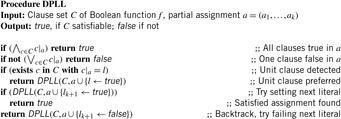
The most popular methods to solve Boolean satisfiability problems are refinements to the Davis-Putnam Logmann-Loveland algorithm (DPLL). DPLL (as shown in Alg. 13.13) is a depth-first variable labeling strategy with unit (clause) propagation. Unit propagation detects literals l in clauses c that have a forced assignment, since all other literals in the clause are false. For a given assignment a we write  for this case. The DPLL algorithm incrementally constructs an assignment and backtracks if this partial assignment already implies that the formula is not satisfiable. Refined implementations of the DPLL algorithm simplify the clauses parallel to the elimination of variables, that proved to be not satisfiable. Moreover, if a clause with only one literal is generated, the literal is preferred and its satisfaction can be propagated through the formula, which can lead to an early backtracking.
There are so many refinements to the basic algorithms that we can only discuss a few. First, we can preprocess the input to allow the algorithms to operate without branching as far as possible. Moreover, preprocessing can help to learn conflicts during the search.
DPLL is sensitive to the selection of the next variable. Many search heuristics have been applied that aim at a compromise between the efficiency to compute the heuristic and the informedness to guide the search process. As a thumb rule, it is preferable not to change the strategy too often during the search and to choose variables that appear often in the formula. For unit propagation we have to know how many literals are not false already. The update of these numbers can be time consuming. Instead, two literals in each clause are marked as observed literals. For each variable x, a list of clauses in which x is true and a list of clauses in which x is false are maintained. If x is assigned to a value, all clauses in its list are verified and another variable in each of these clauses is observed. The main advantage of the approach is that the lists of observables are not updated during backtracking.
Conflicts can be analyzed to determine when and to which depth to backtrack. Such a backjump is a nonchronological backtrack that forgets about the variable assignments that are not in the current conflict set, and has shown consistent performance gains.
As said, the running times of DPLL algorithms depend on the choice/ordering of branching variables in the top level of the search tree. A restart is a reinvocation of the algorithm after spending some fixed time without finding a solution. For each restart, a different set of branching variables can be chosen, leading to a completely different search tree. Often only a good choice of a few variable assignments are needed to show satisfiability or unsatisfiability. This is the reason why rapid restarts are often more effective than continuing the search.
An alternative for solving large satisfiability problems is GSAT, an algorithm that performs a randomized local search. The algorithm throws a coin and performs some variable flips to improve the number of satisfied clauses. If different variables are equally good one is chosen by random. Such and more advanced random strategies are considered in Chapter 14.
Phase Transition
One observation is that many randomly generated formulas are either trivially satisfiable or trivially nonsatisfiable. This reflects a fundamental problem to the complexity analysis of NP-hard problems. Even if the worst case may be hard, many instances can be very simple. As this observation is encountered in several other NP-hard problems, researchers have started to analyze the average case complexity with results much closer to practical problem solving. Another option is to separate problem instances into those that are hard and those that are trivial, and study problem parameters at which (randomly chosen) instances turn from simple to hard or from hard to simple. The change is also known as phase transition. In other words, these instances can be viewed as witnesses for the problem's (NP) hardness. Often it is the case that the phase transition is empirically studied. In some domains, however, theoretical results in the form of upper and lower bounds for the parameters are available.
For Satisfiability, a phase transition effect has been analyzed by looking at the ratio of the number of clauses m and the number of variables n.
The generation of m = αn random formulas in 3-SAT is simple, for example, by a
• random choice of variables, followed by a
• random choice of their signs (positive or negated).
In such random 3-SAT samples, empirically the hard problems have been detected at  . Moreover, the complexity peak (measured in medium computational costs) appeared to be independent to the algorithms chosen. Problems with a ratio smaller than α are underconstrained and easy to satisfy, and problems with a ratio larger than 4.3 are overconstrained and easily shown to be nonsatisfiable.
A simple bound for unsatisfiability is derived as follows. A random clause with three (different) literals according to a fixed assignment a is satisfied with probability 7/8 (only one assignment fails the formula). Therefore, for a fixed assignment a, the entire formula is satisfied with probability  . Given that 2n is the number of different assignments, this implies that the formula is satisfiable with probability
  and unsatisfiable with probability
  . Subsequently, if
  , then the probability for unsatisfiability is larger than 50%. Similar observations have been made for many other problems.
Backbones and Backdoors
The backbone of an SAT problem is the set of literals that are true in every satisfying truth assignment. If a problem has a large backbone, then there are many options to choose an incorrect assignment to the critical variables. Search cost correlates with the backbone size. If the wrong value is assigned to such a critical backbone variable early during the search, the correction of this mistake is very costly. Backbone variables are hard to find.
Theorem 13.5
(Hardness of Finding Backbones) If P ≠ NP, no algorithm can return a backbone literal of a (nonempty) SAT backbone in polynomial time for all formulas.
Proof
Suppose there is such an algorithm. It returns a backbone literal, if the backbone is nonempty. We set this literal to true and simplify the formula. We then call the procedure and repeat. This procedure will find a satisfying assignment if one exists in polynomial time, contradicting the assumption that SAT is NP-hard.
A backdoor into an SAT instance is a set of variables that eases solving the instance. It is weak if the set of variables defines a polynomially satisfiable formula, given a satisfiable instance. It is strong if it gives a polynomially tractable formula for a satisfiable or unsatisfiable problem. For example, there are strong 2-SAT or Horn backdoors. In general, backdoors depend on the algorithm applied, but might be strengthened to the condition that unit propagation will directly solve the remaining problem.
It is not hard to see that that backbones and backdoors are not strongly correlated. There are problems, in which the backbone and backdoor variables are disjoint. However, statistical connections seem to exist. Hard combinatorial SAT problems appear to have large strong backdoors and backbones. Spoken otherwise, the sizes of strong backdoors and backbones are good predictors for the hardness of the problem.
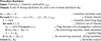
A simple algorithm to calculate backdoors simply tests every combination of literals up to a fixed cardinality. Algorithm 13.14 has the advantage that for small problems, every weak and strong backdoor up to the given size is generated. However, this procedure can only be used for small problems.
13.4.2. Number Partition
The problem of dividing a set of numbers into two parts of equal sums is defined as follows.
Definition 13.7
Let  be a set of numbers, and
  . In Number Partition we search for an index set
  , so that
  .
.
As an example take a = (4, 5, 6, 7, 8). A possible index set is I = {1, 2, 3} since 4 + 5 + 6 = 7 + 8. The problem is solvable only if  is even. The problem is NP-complete, so that we cannot expect a polynomial time algorithm for solving it.
Theorem 13.6
(Complexity Number Partition) Number Partition is NP-hard.
Proof
Number Partition can be reduced from the following (specialized) knapsack problem: Given  and an integer A, decide whether there is a set
  for a
for a  . (Knapsack itself can be shown to be NP-hard by a reduction from SAT.) Given
  as an input for knapsack an instance of Number Partition can be derived as
  . If I is a solution to knapsack then
  is a solution of Number Partition, since
  .
.
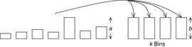
To improve the trivial 2n algorithm for enumerating all possible partitions, we arbitrarily divide the original set of n elements into two of size  and
and  . Then, all subset sums of these smaller sets are computed and sorted. Finally, the two lists are combined in a parallel scan to find value
  .
.
For the example, we generate the lists (4, 6, 8) and (5, 7). The sorted subset sums are (0, 4, 6, 8, 10, 12, 14, 18) and (0, 5, 7, 12) with target value 15. The algorithm takes two pointers i and j; the first one starts at the beginning of the first list and is monotonic increasing, while the second one starts at the end of the second list and is monotonic decreasing. For i = 1 and j = 4 we have 0 + 12 = 12 < 15. Increasing i yields 4 + 12 = 16 > 15, which is slightly too large. Now we decrease j for 4 + 7 = 11 < 15, and increase i twice in turn for 6 + 7 = 13 < 15 and 8 + 7 = 15, yielding the solution to the problem.
Generating all subset sums can be done in time  by full enumeration of all subsets. They can be sorted in time
  using any efficient sorting algorithm (see Ch. 3). Scanning the two lists can be performed in linear time, for the overall time complexity of
  . The running time can be improved to time
  by applying a refined sorting strategy (see Exercises).
Heuristics
We introduce two heuristics for this problem: Greedy and Karmakar-Karp. The first heuristic sorts the numbers in a in decreasing order, and successively places the largest number in the smaller subset. For the example we get the subset sums (8, 0), (8, 7), (8, 13), (13, 13), and (13, 17) for a final difference of 4. The algorithm takes  to sort and O(n) to assign them for a total of
  .
.
The Karmakar-Karp heuristic also sorts the numbers in a in decreasing order. It successively takes the two largest numbers and computes their difference, which is reinserted into the sorted order of the remaining list of numbers. In the example, the sorted list is (8, 7, 6, 5, 4) and 8 and 7 are taken. Their difference is 1, which is reinserted for the remaining list (6, 5, 4, 1). Now 6 and 5 are selected yielding (4, 1, 1). The next step gives (3, 1) and the final difference 2.
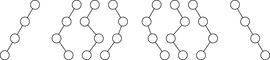
To compute the actual partition, the algorithm builds a tree with one node for each original number. Each operation adds an edge between these nodes. The larger of the nodes represents the difference, so it remains active for subsequent computation. In the example, we have  , with 8 representing difference 1;
  , with 6 representing difference value 1;
  , with 4 representing the difference; and
  with 3 representing the difference. The edges inserted are (8, 7), (6, 5), (4, 8), and (6, 4). The resulting graph is a (spanning) tree on the set of nodes. This tree is to be two-colored to determine the actual partition. Using a simple DFS a two-coloring is available in O(n) time. Therefore, due to the sorting requirement the total time for the Karmakar-Karp heuristic is
  as in the previous case.
Complete Algorithms
The complete greedy algorithm (CGA) generates a binary search tree as follows. The left branch assigns the next number to one subset and the right one assigns it to the other one. If the difference of the two sides of the equation  at a leaf is zero, a solution has been established. The algorithm produces the greedy solution first and continuous to search for better solutions. At any node, where the difference between the current subset sums is greater than or equal to the sum of all remaining unassigned numbers, the remaining numbers are placed into the smaller subset. An optimization is that whenever the two subset sums are equal we only assign a number to one of the lists.
The complete Karmakar-Karp algorithm (CKKA) builds a binary tree from left to right, where at each node we replace the two largest of the remaining numbers. The left branch replaces them by their difference, the right branch replaces them by their sum. The difference is added to the list, as seen before, and the sum is added to the head of the list. Consequently, the first solution corresponds to the Karmakar-Karp heuristic, and the algorithm continues to find better partitions until a solution is found and verified. Similar pruning rules apply as in CGA. If the largest number at a node is greater than the subset sum of the others, it can be safely pruned.
If there is no solution, both algorithms have to traverse the entire tree, such that the algorithms perform equally bad in the worst case. However, CKKA produces better heuristic values and better partitions. Moreover, the pruning rule in CKKA is more effective. For example, in CKKA (4, 1, 1) and (11, 4, 1) are the successors of (6, 5, 4, 1), and the largest number is greater than the sum of the others, so that both branches are pruned. In CGA, the two children of the subtrees with difference 5 and difference 7 have to be expanded.
13.4.3. *Bin Packing
Definition 13.8
(Bin Packing) Given n objects of size  the task in Bin Packing is to distribute them among the bins of size b in such a way that a minimal number of bins is used. The corresponding decision problem is to find a mapping
  for a given k such that for each j the sum of all objects ai with
  is not larger than b.
Here we see that optimization problems are identified with corresponding decision problems, thresholding the objective to be optimized to some fixed value.
Theorem 13.7
(Complexity of Bin Packing) The decision problem for Bin Packing is NP-hard.
Proof
NP-hardness can be shown using a polynomial reduction from Number Partition. Let  be the input of Number Partition. The input for Bin Packing is n objects of size
  and
and  . If
. If  is odd, then Number Partition is not solvable. If
  is even and the original problem is solvable, then the objects have a perfect fit into the two bins of size A.
There are polynomial-time approximation algorithms for Bin Packing like first fit (best fit and worst fit), which incrementally searches for the first (best, worst) placement of an object in the bins (the quality of the fit is measured in terms of the remaining space). First fit and best fit are known to have an asymptotic worst-case approximation ratio of 1.7, by means that they cannot generally produce solutions that are better than 1.7 times the optimum in the limit for large optimization values.
The modifications first fit decreasing and best fit decreasing presort the objects according to their size. The rationale is that starting with the larger objects first will be better than having them be placed at the end. Postponing the smaller ones, we can expect a better fit. Indeed using a decreasing order of object sizes together with either strategy first fit or best fit can be shown to guarantee solutions that are at most a factor of 11/9 off from the optimal one. Both algorithms run in  time.
time.
Bin Completion
The algorithm for optimal Bin Packing is based on depth-first branch-and-bound (see Ch. 5). The objects are first sorted in decreasing order. The algorithm then computes an approximate solution as initial upper bound, using the best solution among first fit, best fit, and worst fit decreasing. The algorithm next branches on the different bins in which an object can be placed.
The bin completion strategy is based on feasible sets of objects with a sum that fits with respect to the bin capacity. Rather than assigning objects one at a time to bins, it branches on the different feasible sets that can be used to complete each bin. Each node of the search tree, except the root node, represents a complete assignment of objects to a particular bin. The children of the root represent different ways of completing the bin containing the largest object. The nodes at the next level represent different feasible sets that include the largest remaining object. The depth of any branch of the tree is the number of bins in the corresponding solution.
The key property that makes bin completion more efficient is a dominance condition on the feasible completions of a bin. For example, let A = {20, 30, 40} and B = {5, 10, 10, 15, 15, 25} be two feasible sets. Now partition B into the subsets {5, 10}, {25}, and {10, 15, 15}. Since 5 + 10 ≤ 20, 25 ≤ 30, and 10 + 15 + 15 ≤ 40, set A dominates set B.
To generate the nondominated feasible sets efficiently we use a recursive strategy illustrated in Algorithm 13.15. The algorithm generates feasible sets and immediately tests them for dominance, so it never stores multiple dominated sets. The inputs are sets of included, excluded, and remaining objects that are adjusted in the different recursive calls. In the initial call (not shown) the set of remaining elements is the set of all objects, while the other two sets are both empty. The cases are as follows. If all elements have been selected or rejected or we have a perfect fit, we continue with testing for dominance, otherwise we select the largest remaining object. If it is oversized with respect to remaining space we reject it. If it has a perfect fit we immediately include it (the best fit for the bin has been obtained) and continue with the rest; in the other cases we check for both inclusion and exclusion. Procedure Test checks dominance by comparing subset sums of included elements to excluded elements rather than comparing pairs of sets for dominance. The worst-case running time of procedure Feasible is exponential, since by reducing set R we obtain the recurrence relation  .
.
Improvements
To improve the algorithm there are different options. The first idea is forced placements that reduce the branching. If only one more object can be added to a bin, which is easy to be checked by scanning through the set of remaining elements, then we only add the largest of such objects to it, and if only two more objects can be added, we generate all undominated two-element completions in linear time.
For pruning the search space, we consider the following strategy: Given a node with more than one child, when searching the subtree of any child but the first, we do not need to consider bin assignments that assign to the same bin all the objects used to complete the current bin in a previously explored child node. One implementation of this rule propagates a list of no-good sets along the tree. After generating the undominated completions for a given bin, we check each one to see if it contains any current no-good sets as a subset. If it does, we ignore that bin completion. The list of no-goods is pruned as follows. Whenever there is a no-good set, but the no-good set is not a subset of the bin completion, we remove that no-good set from the list that is passed down to the children of that bin completion. The reason is that by including at least one but not all the objects in the no-good set, we guarantee that it cannot be a subset of any bin completion below that node in the search tree.
13.4.4. *Rectangle Packing
Rectangle Packing considers packing a set of rectangles into an enclosing rectangle. It is not difficult to devise a binary CSP for the problem. There is a variable for each rectangle, the legal values of which are the positions it could occupy without exceeding the boundaries of the enclosing rectangle. Additionally, we have a binary constraint between each pair of rectangles that they cannot overlap.
Definition 13.9
(Rectangle Packing) In the decision variant of the Rectangle Packing problem we are given a set of rectangles ri of width wi and height hi,  and an enclosing rectangle of width W and height H. The task is to find an assignment to all the left upper corner coordinates
  of all rectangles ri such that
• each rectangle is entirely contained in the enclosing rectangle; that is, for all  we have
  ,
,  ,
,  , and
, and  .
.
• no two rectangles ri and rj with  overlap; that is,
The optimization variant of the rectangle problem asks the smallest enclosing rectangle for which an assignment to the variable is possible.
When placing unoriented rectangles, both orientations are to be considered.
Rectangle Packing is important for VLSI and scheduling applications. Consider n jobs, where each job i requires a number of machines mi and a specific processing time di,  . Finding a minimal-cost schedule is equivalent to Rectangle Packing with
  and
and  for
for  .
.
Theorem 13.8
(Complexity Rectangle Packing) The decision problem for Rectangle Packing is NP-hard.
Proof
Rectangle Packing can be polynomially reduced from Number Partition as follows. Assume we have an instance of number partition . Now we create an instance for Rectangle Packing as follows. First we choose an enclosing rectangle with width W and height
  . If
. If  is odd then there is no possible solution to Number Partition. (W is chosen small enough to disallow changing orientation of the rectangle.) The rectangles to be placed have width W ∕ 2 and height ai. Since the entire space of
  cells has to be covered, any solution to the Rectangle Packing problem immediately provides a solution to the Number Partition. If we do not find a solution to the rectangle packing problem it is clear that there is no partitioning of a into two sets of equal sum.
In the following we concentrate on rectangles of integer size. As an example, Figure 13.18 shows the smallest enclosing rectangle for 1 × 1 to 25 × 25. This suggests an alternative CSP encoding based on cells. Each cell cij with  and
and  corresponds to a finite-domain variable
  , which denotes if the cell cij is free (0) or the index of the rectangle that is placed on it. To check for overlapping rectangles, a two-dimensional array representing the actual layout of cells is used. When placing a new rectangle we only need to check if all cells on the boundary of the new rectangle are occupied.
Wasted Space Computation
As rectangles are placed, the remaining empty space gets chopped up into smaller irregular regions. Many of these regions cannot accommodate any of the remaining rectangles and must remain empty. The challenge is to efficiently bound the amount in a partial solution.
A first option for computing wasted space is to perform horizontal and vertical slices of the empty space. Consider the example of Figure 13.19. Suppose that we have to pack one (1 × 1) and two (2 × 2) rectangles into the empty area. Looking on the vertical strips we find that there are five squares that can only accommodate the squares (1 × 1), such that 5 − 1 = 4 squares have to remain empty. On the other hand, 11 − 4 = 7 squares are not sufficient to accommodate the three rectangles of total size 9.

The key idea to improve the wasted space calculation is to consider the vertical and horizontal dimensions together rather than performing separate calculations in the two dimensions and taking the maximum. When packing oriented rectangles we have at least different choices for computing wasted space. One is to use our new lower bound that integrates both dimensions but using the minimum dimension of each rectangle to determine where it can fit. Another option is to use the new bound but use both the height and width of each empty rectangle.
For each empty cell, we store the width of the empty row and the height of the empty column it occupies. In an area of free cells, empty cells are grouped together if both values match. We refer to these values as the maximum width and height of the group of empty cells. A rectangle cannot occupy any of a group of empty cells if its width or height is greater than the maximum width or height of the group, respectively. This results in a Bin Packing problem (see Fig. 13.20). There is one bin for each group of empty cells with the same maximum height and width. The capacity of each bin is the number of empty cells in the group. There is one element for each rectangle to be placed, the size of which is the area of the rectangle. There is a bipartite relation between the bins and the elements, specifying which elements can be placed in which bins, based on their heights and widths. These additional constraints simplify the Bin Packing problem. For example, if any rectangle can only be placed in one bin, and the capacity of that bin is smaller than the area of the rectangle, then the problem is unsolvable. If any rectangle can only be placed in one bin, and the capacity of the bin is sufficient to accommodate it, then the rectangle is placed in the bin, eliminated from the problem, and the capacity of the bin is decreased by the area of the rectangle. If any bin can only contain a single rectangle, and its capacity is greater than or equal to the area of the rectangle, the rectangle is eliminated from the problem, and the capacity of the bin is reduced by the area of the rectangle. If any bin can only contain a single rectangle, and its capacity is less than the area of the rectangle, then the bin is eliminated from the problem, and the remaining area of the rectangle is reduced by the capacity of the bin.
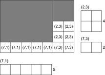
Considering again the example of packing one (1 × 1) and two (2 × 2) rectangles, we immediately see that the first block can accommodate one (2 × 2) rectangle, but the second (2 × 2) rectangle has no fit.
Applying any of these simplifying rules may lead to further simplifications. When the remaining problem cannot be simplified further, we compute a lower bound on the wasted space. We identify a bin for which the total area of the rectangles it could contain is less than the capacity of the bin. The excess capacity is wasted space. The bin and the rectangles involved are eliminated from the problem. We then look for another bin with this property. Note that the order of bins can affect the total amount of wasted space computed.
Dominance Conditions
The largest rectangle is placed first in the top-left corner of the enclosing rectangle. Its next position will be one unit down. This leaves an empty strip one unit high above the rectangle. While this strip may be counted as wasted space, if the area of the enclosing rectangle is large relative to that of the rectangles to be packed, this partial solution may not be pruned based on wasted space. Partial solutions that leave empty strips to the left, of or above rectangle placements are often dominated by solutions that do not leave such strips, and hence can be pruned from considerations (see Fig. 13.21).

A simple dominance condition applies whenever there is a perfect rectangle of empty space of the same width immediately above a placed rectangle, with solid boundaries above, to the left, and to the right. The boundaries may consist of other rectangles or the boundary of the enclosing rectangle. Similarly, it also applies to a perfect rectangle of empty space of the same height immediately to the left of a placed rectangle.
13.4.5. *Vertex Cover, Independent Set, Clique
For the next set of NP-hard problems we are given an undirected graph  . The problems Vertex Cover, Clique, and Independent Set are closely related.
Definition 13.10
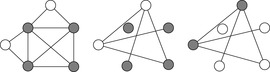
(Vertex Cover, Clique, Independent Set) In Vertex Cover we are asked to find a node subset V′ such that for all edges in E at least one of the end nodes is contained in V′. Given G and k, Clique decides, whether or not there is a subset  such that for all
  we have
  . Clique is the dual to the Independent Set problem, which searches for a set of k nodes that contains no edge connecting any two of them.
An illustration for the three problems is provided in Figure 13.22.
 |
| Figure 13.22 |
Theorem 13.9
(Complexity Vertex, Cover, Clique, Independent Set) Vertex Cover, Clique, and Independent Set are NP-hard.
Proof
For Clique and Independent Set, we simply have to invert edges to convert the problem instances. To reduce Independent Set to Vertex Cover, we take an instance  and k to Independent Set and let the Vertex Cover algorithm run on the same graph with bound n − k. An independent set with k nodes implies that all other n − k nodes supervise all edges. Otherwise, if n − k nodes cover the edge set, then all other k nodes build an independent set.
Therefore, we only have to show that one of the three graph problems is NP-hard. This can best be done using a reduction of 3-SAT to Clique. Given a 3-SAT formula C consisting of the m clauses  , the input for Clique is defined as follows: V contains 3m nodes labeled by the pair
  . Nodes represent the variables in the clauses. Set E contains an edge between
  and
and  if
if  and the literal corresponding to
  is not negated at
  . Value k is set to m. It is easy to see that we have a satisfying assignment for C if and only if the selected nodes form a clique of size k.
Given these equivalences, from now on, we discuss only Vertex Cover.
Enumeration
For search algorithms on graphs it is important to clarify terms. We distinguish between nodes in the search tree and vertices in the graph. A brute-force approach enumerates all 2n different subsets and finds the smallest one that is a vertex cover. A search tree is built with internal nodes corresponding to partial assignments that branch on whether vertices are in V′ or not, and the leaves corresponding to a complete assignment. Spanning a binary search tree of included and excluded vertices, the check of a vertex performed incrementally by traversing the tree, yields an  algorithm. For a partial assignment we have three sets: the set of included, the set of the excluded, and the set of free vertices.
A first improvement is to eliminate vertices u of degree one, while moving adjacent vertices v of u to the vertex cover. A more general observation is that if a node is not included in the vertex cover then all of its neighbors have to be included in the vertex cover. This will lead to forced assignments. The opposite idea is to eliminate all edges of a node that is selected, since they are already covered. During the search process this may lead to isolated free vertices that have to be included into the cover, or ones of degree one that are excluded with its neighbors included. Another improvement is to order the nodes in the search tree with respect to decreasing node degree. Nodes with many neighbors will be found high up in the search tree, while nodes with only a small number of neighbors are found to its bottom.
Lower Bounds
When looking at individual vertices in the free graph (the remaining graph that is induced by the not yet assigned nodes) there is not much to infer. But by looking at pairs of vertices we can devise a nontrivial heuristic as follows. For each pair of nodes  from the free graph we define the admissible pairwise cost 1, if
  , and 0 otherwise. This yields a bipartite graph. Since we look for edges with both endpoints that are not in the vertex cover, we are computing a maximum matching of the free graph, which can be computed in polynomial time.
13.4.6. *Graph Partition
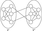
Definition 13.11
(Graph Partition Problem) In Graph Partition a graph G has to be divided into two equal-size sets of vertices  with
with  and
and  such that the number of edges
  that go from one set to the other is minimized. The decision variant (a.k.a. minimum-cut problem) takes an additional parameter k, and asks whether or not
  .
.
The problem is very relevant in practice. Probably the most important application is parallel processing in a computer network. Given n tasks and p processors (here p = 2), there are many ways to assign n tasks to p processors, some of which have a low and some of which have a high communication overhead.
Theorem 13.10
(Complexity Graph Partition) Graph Partition is NP-hard.
Proof
We show that Graph Partition can be reduced from Simple Max Cut. This problem is known to be NP-hard by a polynomial reduction from 3-SAT (see Exercises) and defined as follows. Given a graph and an integer k the question is if there is a set N such that  .
.
For an input  of Simple Max Cut we construct an input
  for Graph Partition as follows:
  , with
  ,
,  , and
, and  . Suppose there is a partition
  such that
  . Since k > 0 we have
  and
and  . Let
. Let  ,
,  , and
, and  , then
  is a partition of
  with
with  ,
,  ,
,  , and
, and Now suppose that there is a partition W′ and W′′ with
  ,
,  , and
, and  such that
  . Then
  where
where  and
and  is a partition of
  such that
 Therefore, G has a cut of size greater than or equal to k if and only if G∗ has a partition into equal-size subsets with less than k∗ edges.
If no restriction to the size of the subsets is made, the problem can be solved in polynomial time (this is the famous max-cut or min-flow problem). However, other variants of Graph Partition are also NP-hard. The problem of dividing the vertices into an arbitrary number of sets with at most M vertices per set is NP-hard even when M = 3. If M = 2, it is not hard to see that the problem is equivalent to maximum matching.
In some variants of Graph Partition edge weights are introduced. An application for such extended domain is VLSI design, where the vertices are logical units on the chip, and the edges are wires connecting them. The goal is to place the units on the chip so as to minimize the numbers and lengths of the wires connecting them. In Gaussian elimination, graph partition can be used to reorder the rows and columns of the matrix to decrease the number of nonzero entries created during elimination.
Nodes in the search tree correspond to partial graph partitions of some of the vertices. At each such node, the left branch corresponds to an assignment of a vertex to V′ and on the right branch we assign the same vertex to V′′. It is obvious that the search tree is binary and has depth n − 1. We are only interested in leaves that partition the vertices into equal-size subsets. When pruning nodes with either  or
or  we have
  leaves remaining in the search tree.
Heuristics
Vertices not being assigned are called free vertices. Heuristic function proposes different completion strategies. Therefore, we distinguish between the assignment of vertices in V′ (group A), the assignment of vertices in V′′ (group B), the proposed completion to V′(group A′), and the proposed completion to V′′ (group B′).
We can divide the edges in the graph into four types:
1. Edges within A and A′ or within B and B′ do not cross the partition and will not be counted by any heuristic.
2. Edges from A to B are already crossing the partition.
3. Edges from A′ to B or from B′ to A connect free to assigned vertices.
4. Edges from A′ to B′ connect free vertices (see Fig. 13.24).
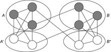
The number of direct edges that connect a free vertex x to A (or B) is denoted by  (or
(or  ). In the following we present two different heuristic functions for the Graph Partition problem.
For each free vertex let  . For a search node u we define
  as the sum of
  for all free vertices in u. We observe that up to the tie-breaking function
  implicitly selects an appropriate set for each free variable x.
Let x and y be a pair of free vertices connected by an edge; then we define  ,
,  . It is a lower bound on the number of edges that must cross the partition. To compute
  for a search node u we have to combine the values
  for the free variables. This is done as follows. All pairwise distances are included into a pair graph, where an edge between x and y is weighted with
  . Once more, a maximal matching is used to avoid that the influence of a free variable is counted more than once. To improve the running time from cubic to quadratic, during the search process the maximal matching can be computed incrementally. Unfortunately, this heuristic turns out to be too complicated in practice. It is, however, effective to improve the heuristics by drawing inferences on the free graph that connects free vertices in A′ and in B′(see Exercises).
Search Enhancements
The first option to enhance the search process that is similar to a strategy in Bin Packing is to sort the vertices of the graph in decreasing order of degree and add new vertices to that order rather than taking a random order. The reason is that if we handle nodes with large branching factors at the top of the search tree then we have more flexibility for selecting sets in larger depth. This extension improves both IDA* and depth-first branch-and-bound.
Most of the nodes generated at the bottom of the search tree get pruned, and some of the heuristics are more complicated than others. Therefore, it is often effective first to check computationally simpler heuristics to detect failure, instead of selecting only the involved ones. For the graph partition problem this reduces the average time per node by more than 20% in practice.
13.5. Temporal Constraint Networks
A temporal constraint network consists of a set of variables  that denotes time points. It is a special case for CSP s with real-valued variables. Each constraint can be interpreted as a set of (closed) intervals
  .
.
A unary constraint C(i) bounds the range of variables xi to the disjunction of  , …,
, …,  , and a binary constraints
  bounds the range of the difference
  to the disjunction of
  , …,
, …,  . We implicitly assume that conditions are on pairwise different intervals.
A binary constraint network consists only of unary and binary constraints. It is interpreted as a constraint graph  , where V denotes the set of variables and E is defined by the constraints. Edges are annotated with the intervals that are in the corresponding constraints. A solution of a temporal CSP is an assignment to variables that satisfies all constraints.
A minimal constraint network is a constraint network where all intervals are minimal. It turns out that the decisions, if a network obeys a solution, and the task to determine possible assignment to xi are NP-hard. Consequently, we have to work on polynomial subclasses. In the following we will see how to restrict the network to perform a consistency check and to compute the minimal network in  time.
time.
The restriction we apply is to use at most one time interval for each pair of variables. This way, we disallow disjunctive conditions. Solving this simple temporal network subproblem also gives an algorithm for the overall problem via the application of branch-and-bound, where branching is obtained by selecting or neglecting one interval for a given edge. Let l be the number of edges in the constraint graph, and k be the maximal number of disjuncts at one edge. Having  time to solve one simple temporal network, we subsequently require
  time to obtain a solution for the disjunctive temporal constraint network (for each edge there are k options to choose from, so that k determines the branching factor in a search tree of depth l spanned by the constraints).
13.5.1. Simple Temporal Network
In a simple (temporal) constraint network all constraints are either of the form  or
or  . The first form refers to a binary constraint and the second form corresponds to a unary constraint. Unary constraints can be eliminated by introducing an additional partner variable forced to be zero. Therefore, we arrive at a linear program with a simple structure. Referring to variables as time points, the set of constraints in a simple temporal network denote time intervals. As an example consider the following set of constraints:
  ,
,  ,
,  ,
,  ,
,  ,
,  ,
,  ,
,  ,
,  , and
, and  .
.
In a weighted distance graph we associate weights to the edges of a graph, where each node represents a variable. The value  represents the inequality
  . The weighted distance graph for the example constraint set is shown in Figure 13.25. Consequently, for each path
  to
to  via nodes
  we have
 Since there are several paths from i to j we have
  , where
  is the minimum over
  . Each negative cycle
  corresponds to unsatisfiable inequality
  .
.
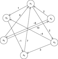
Theorem 13.11
(Consistency Simple Temporal Network) A simple temporal constraint network is consistent if the distance graph contains no cycles.
Proof
We start with a distance graph with no negative cycles. Henceforth, there exists a shortest path between every two connected nodes. For shortest path costs δ we have  or
or  . Hence, the assignment
  to the variables
  is a solution to the temporal network.
Moreover, we have that  is a solution and corresponds to the latest and earliest point in time. The minimal temporal constraint network is defined by constraints
  . The set of possible assignments to xi is defined by
  . The constraint network is inconsistent if we have
  for one index i.
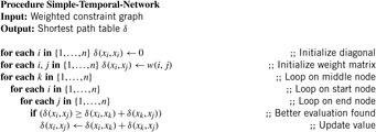
By the posterior calculations, the consistency problem is solved in  with a variant of the All-Pairs Shortest Path problem of Floyd and Warshall. Although the algorithm does not differ much from the presentation in Chapter 2, we have included the pseudo code of Algorithm 13.16.
13.5.2. *PERT Scheduling
The project evaluation and review technique (PERT) is a method to determine critical paths in project scheduling. We are given a set of operators O together with a precedence relationship among them. A simple example is provided in Figure 13.26. Let  be the earliest end time of oi and
  be the duration of oi; then the earliest starting time is
  .
.

The critical path is a sequence of operators, such that their total running time is greater than or equal to all other operator path costs. Any delay on the critical path enforces a delay within the project. The heart of the PERT scheduling problem is a network of operators, together with the precedence relationship  , where
  means that the end time of oi is less than or equal to the start time of oj.
Algorithmically, PERT scheduling can be seen as a shortest path algorithm for acyclic graphs. It is well known that an acyclic graph can be topologically sorted in linear time. This induces that a node is processed only if all its predecessors have been processed. Viewed from a different angle, PERT scheduling can be interpreted as a specialized instance of a simple temporal constraint network, since we can model start and end times of each operator as time intervals using two constraint variables and the precedence relation as a binary constraint. The main advantage is that precedence scheduling problems can be solved roughly in quadratic time, whereas simple temporal network analysis requires cubic time. The pseudo code is shown in Algorithm 13.17.
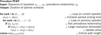
Theorem 13.12
(Optimality and Time Complexity PERT Scheduling) The schedule  defined by the PERT algorithm is optimal and can be computed in time
  , where l is the number of preferences induced by
  .
.
Proof
The induction hypothesis is that after iteration i, the value of  is correct. For the base case, this is true, since
  . For the step case, we assume the hypothesis to be true for
  . There are two cases.
1. There exists  with
with  . Hence,
  . The value of
  is optimal, since oi cannot start earlier as
  given that all
  are the smallest possible.
2. There is no  with
with  . Therefore,
  as in the base case.
To summarize, the value  is the duration of an optimal schedule.
To compute  we determine the earliest start times by setting set
  ,
,  . The time complexity of the algorithm is
  , which can be reduced to
  using adjacency lists.
13.6. *Path Constraints
Path constraints provide an important step toward the description of temporally extended goals and have also been used to prune the search in the form of additionally extended control knowledge. In short, path constraints assert conditions that must be satisfied during the execution of the sequence of states visited during the execution of a solution path. Path constraints are often expressed through temporal modal operators. Basic modal operators are always, sometime, at-most-once, and at end (for goal constraints). The set is extended with within, which can be used to express deadlines. In addition, conditions like sometime-before and sometime-after indicate the option of operator nesting. For a solution path  , such constraints are interpreted as illustrated in Figure 13.27, where ⊧ is chosen as the derivation symbol.

All these conditions can be combined with Boolean operators ∧, ∨, ¬ to generate more complex expressions. In a more general setting, path constraints are expressed in linear temporal logic (LTL). LTL is a propositional logic over Boolean operators and includes arbitrary nesting of the temporal modalities.
LTL is defined on the notion of infinite paths in model M, which is a sequence of states  . Moreover, let πi for i > 0 denote the suffix of π starting at ui.
Definition 13.12
(Syntax and Semantics of LTL) LTL formulas have the form always f, Af for short, where f is a path formula. If p is an atomic proposition then p is a path formula. If f and g are path formulas then  are path formulas.
For the next-time operator X we have  . For the until operator g U f we have
  . For the eventually operator we have
  . For the globally operator we have
  .
.
We give the following three examples (see Fig. 13.28).

1. The LTL formula A(G p) means along every path, p will hold forever.
2. The LTL formula A(F p) means along every path, there is some state in which p will hold.
3. The LTL formula A(FG p) means along every path, there is some state from which p will hold forever.
For performing heuristic search on the extended plan conditions, we have to be able to evaluate the truth of the constraints on-the-fly for each encountered state. There have been two suggestions being made to associate the formula with the currently expanded state.
13.6.1. Formula Progression
One option to use LTL formulas for constraint search is formula progression. Depending on the structure of an LTL formula f a procedure Progress (see Alg. 13.18) propagates the satisfaction of f from a state to its successor.
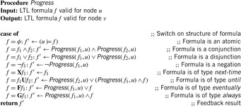
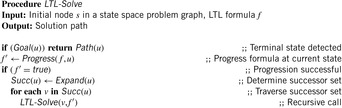
As a running example we take Blocksworld. Suppose we want to propagate G (on a b) in a node for which we know that (on a b) is satisfied. We obtain a formula true ∧ G (on a b), which further simplifies to G (on a b). If (on a b) is not satisfied, we obtain false ∧ G (on a b), also false.
We briefly discuss a forward-chaining search algorithm that takes LTL control rules to prune the search tree. With each node in the search tree we associate a formula. When expanding a node u the associated formula fu is progressed to the successor v. The pseudo code is shown in Algorithm 13.19. For the sake of simplicity we have chosen a depth-first search traversal, but the algorithm extends to any kind of search algorithm (see Exercises).
It is not difficult to see that if the algorithm LTL-Solve terminates at a node u with associated  , no successor will ever fulfill the imposed constraint (see Exercises).
Integrating a search heuristic to the LTL-Solver is not immediate. However, if we are able to determine a measurement on how far a temporal formula is from its satisfaction, we could order the states along this measurement to prefer the ones that are closer to it.
13.6.2. Automata Translation
LTL formulas are often translated into an equivalent automata that runs concurrently to the transitions taken in the overall search process and that accept when the constraint is satisfied. As LTL formulas have been designed to express properties of infinite paths the automaton models are Büchi automata. Syntactically, Büchi automata are the same as finite-state automata, but designed for the acceptance of infinite words. They generalize the finite case by having a slightly different acceptance condition. Let ρ be an infinite path and  be the set of states reached infinitely often in ρ; then a Büchi automaton accepts, if the intersection between
  and the set of final states F is not empty. Because the paths are finite, we can view the Büchi automaton as an ordinary nondeterministic finite-state automaton, which accepts a word if it terminates in a final state. The labels of the automaton are conditions on the set of variables in a given state. For a more detailed treatment of searching with Büchi-Automata we refer the reader to Chapter 16.
Every LTL formula can be transformed into an equivalent Büchi automaton. (The contrary is not always possible, since Büchi automata are clearly more expressive than LTL expressions.) The application of automata in the search is that they run concurrent to the ordinary state exploration (each operator in the original state space induces a transition in the automaton). If the automaton accepts the LTL formula ϕ from which the automaton has been built, ϕ is fulfilled. As there are many elaborated tools for the nontrivial transformation of LTL expressions into automata representation, we do not dwell on how to derive the automaton construction automatically. Instead, we provide some examples.
For (sometimeϕ) with respect to some constraint ϕ, an automaton for the LTL formula Fϕ is built. Let S be the original state space and AFϕ be the constructed automaton for formula AFϕ and ⊗ denote the interleaved (synchronous) cross-product between the state space and the automaton, then the combined state space is S ⊗ AFϕ with extended goal T ⊗ {accepting(AFϕ)}. The initial state s of the search problem is extended by the initial state of the automaton, which in this case is not accepting.
As an example consider the Blocksworld assertion that on every solution path two blocks a and b should be put down on the table at least once. This requirement corresponds to the LTL formula  with a Büchi automaton shown in Figure 13.29 (left, && corresponds to ∧). The statement in some state visited by the plan both blocks a and b are on the table is expressed in LTL formula as
  with a Büchi automata shown in Figure 13.29 (right).
For formulas like  we construct the cross-product
  For nested expressions like
  the temporal formula is more complicated, but the reasoning remains the same. We set
 and adapt the goal and the initial state accordingly.
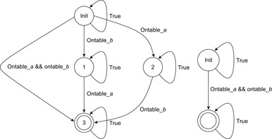 |
| Figure 13.29 |
For (at-most-once ϕ) we explore the combined state space  and for (within t ϕ) we first build the cross-product
  as for sometime. Additionally, we enforce
  to be fulfilled already in step t.
Constructing the Büchi automaton prior to the search can be a time-consuming task. However, the savings during the search are considerable, as for each state in the search space it only has to store and progress the state in the automaton instead of the formula description as a whole.
Concerning heuristics for the extended state spaces, it is not difficult to extend a distance heuristic for the original state space without the constraints with distance to an accepting state in the Büchi automaton. In other words, the minimum distance to an accepting state in the automaton is another admissible heuristic for finding a valid solution to the original problem. The state-to-accepting-state distances can be computed by invoking All-Pairs Shortest Paths in the automaton or by chaining backward from the goal (as in pattern databases).
13.7. *Soft and Preference Constraints
Annotating goal conditions and temporal path constraints with preferences models soft constraints. A soft constraint is a condition on the trajectory generated by a solution that the user would prefer to see satisfied rather than not satisfied, but is prepared to accept not satisfying it because of the cost of satisfying it, or because of conflicts with other constraints or goals. In case a user has multiple soft constraints, there is a need to determine which of the various constraints should take priority if there is a conflict between them or if it should prove costly to satisfy them.
For example, in Blocksworld we might prefer block a to reside on the table if a goal is reached. In a more complex transportation task we might want that whenever a ship is ready at a port to load the containers it has to transport, and all such containers should be ready at that port. Moreover, at the end we would prefer all trucks to be clean and to be present at their source location. Additionally, we would like no truck to visit any destination more than once.
Such preference constraints are included into the cost or objective function. This function calls for searching cost-optimal plans.
Goal preferences refer to constraints that are added to the goal condition. For example, if we prefer block a to reside on the table during the plan execution, we may impose preference p (on-table a) with a indicator variable isviolatedp (denoting the violation of p) to be included in an objective function. Such indicators are interpreted as natural numbers that can be scaled and combined with other variable assignments in the objective function. More precisely, if we have a soft constraint of type  , we construct the indicator function
  and include isviolatedp as a variable into
  , which has to be minimized.
Preferences for plan constraints can, in principle, be dealt with automata theory. Instead of requiring to reach an accepting state we prefer to be there, by means that not arriving at an accepting state incurs costs to the evaluation of the objective function.
There is, however, a subtle problem. Because trajectory constraints may prune the search, a preference violation can also be due to a failed transition in the automata. For example, the constraints like  prunes the search on each operator in which the only transition is not satisfied. The solution to this problem is to introduce extra transitions (one for each automata) that allow the enforced synchronization to be bypassed. Applying this transition is assigned to the corresponding costs and forces the automata to move into a dead(-end) state, from which there is no way back to any other automata state.
13.8. *Constraint Optimization
The option for constraint optimization on top of constraint satisfaction is realized via a function that has to be minimized or maximized. Because we can negate the objective function, we can restrict constrained optimization to the minimization of an objective function subject to constraints on the possible values for the constraint variables. Constraints can be either equality constraints or inequality constraints.
The typical constrained optimization problem is to minimize some cost function f(x) subject to constraints of the form  or
or  . Function f is called the (scalar-valued) objective function and g and h are the vector-valued constraint functions. Strict convexity of the objective function is not sufficient to guarantee a unique minimum. In addition, each component of the constraint must be strictly convex to guarantee that the problem has a unique solution. In fact, solutions to the constrained problem are often not stationary points. Consequently, ad hoc techniques of searching for all stationary points that also satisfy the constraint do not work.
If we restrict the class of constraint and objective functions we can do much better. If we take linear constraints, depending on the domain of x this corresponds to either a linear program (LP) or integer linear program (ILP). While LP is polynomial time solvable, IP is NP-complete also for the case if the input variables x are either 0 or 1. Here we restrict integer programming concerning the satisfiability of a conjunction of linear constraints on integer variables. Constraint optimization problems on more general formalisms are considered in Chapter 14.
The efficiency of constraint processing is dependent on the representation of the constraint. A recent trend is to use BDDs (see Ch. 7) for bounded arithmetic constraints and linear expressions.
To compute a BDD F(x) for a linear arithmetic function  , we first compute the minimal and maximal value that f can take. This defines the range that has to be encoded in binary.
For the ease of presentation, we consider  . This restriction is sufficient to deal with goal preferences as introduced earlier.
Theorem 13.13
(Time and Space Complexity Linear Arithmetic Constraint BDDs) The BDD for representing f has at most  nodes and can be constructed with matching time performance.
Proof
For the construction, the BDD is interpreted as a serial processor that processes the integer variables  in this order. In the end the processor verifies whether or not
  or
or  . If at any time the computation fails the BDD immediately evaluates to zero. Otherwise it continues. The processing starts with an initial value of
  and then gradually adds
  for increasing
  . How many BDD nodes are needed in each level? The number can be bound by the range of the partial sum of all coefficients considered so far. This implies that the total number of nodes in the BDD is at most
  as stated.
The approach extends to integer variables xi,  with
with  and to the conjunction/ disjunction of several linear arithmetic formulas (see Exercises). This implies that integer programming on the satisfiability of a conjunction of m linear constraints can be solved in time
  . The algorithm is polynomial in n and b but exponential in m, the number of constraints. If n can be fixed then a pseudo-polynomial algorithm exists.
13.9. Summary
A (hard) constraint is a restriction on the solution of a search problem. Generic constraint satisfaction problems (CSPs) consist of a set of variables that need to get assigned a value each from their discrete domains, say one of the values red, green, or blue. The constraints impose restrictions on the possible assignments, for example, that variable X cannot be assigned red if variable Y is assigned green. An example of a CSP is map coloring, where we need to pick a color for every state from among three available colors so that neighboring states receive different colors. We showed how constraints that involve three or more variables can be transformed to constraints that involve only one variable (unary constraints) or two variables (binary constraints). We then discussed different search methods for the resulting CSPs.
The idea behind constraint propagation is to rule out certain assignments to make the subsequent search more efficient. Arc consistency rules out a value x for a variable X if the variable is involved in at least one binary constraint that cannot be satisfied if variable X is assigned value x. (If the values are integers, arc consistency can maintain intervals of values rather than sets of values and is then also referred to as bounds consistency.) Path consistency is more powerful than arc consistency by checking paths of constraints at the same time instead of only individual constraints; for example, a binary constraint between variables X and Y and a binary constraint between variables Y and Z. It is sufficient to check paths of length two. There are also specialized consistency methods, such as the constraint that all variables need to be assigned pairwise different values.
Constraint propagation methods rarely result in only one possible value for each variable. Thus, they do not eliminate the need for search. The simplest possible systematic search method is backtracking; that is, depth-first search. (We will discuss randomized search in Chapter 14.) Backtracking assigns values to the variables one after the other in a fixed order and backtracks immediately if a partial assignment violates some constraint. There are several ways of making backtracking more efficient. Backjumping improves on backtracking by backtracking to the variable that is responsible for the constraint violation instead of the previous variable. Dynamic backtracking improves on backjumping by not forgetting the assignments to the variables between the current one and the one to which it backtracks. Backmarking improves on dynamic backtracking by removing additional constraint checks.
Various heuristics have been studied to decide in which order the various backtracking methods should consider the variables and in which order they should consider the values of the variables (i.e., variable and value ordering). However, it can be inefficient to consider the values of the variables in a fixed order since, after some backtracks, the assignments of values to variables can differ substantially from the ones recommended by the heuristic. It is called a discrepancy to not assign a variable the value recommended by the heuristic. Limited discrepancy search uses the backtracking methods to generate complete assignments of values to variables to increase the number of discrepancies. The simplest version of limited discrepancy search generates in its i th iteration all complete assignments of values to variables with at most i − 1 discrepancies and thus replicates the effort of its (i − 1)th iteration. Improved limited discrepancy search improves on limited discrepancy search by using a user-provided depth limit to generate in its i th iteration all complete assignments of values to variables with exactly i − 1 discrepancies. Often, the heuristic is less reliable toward the top of the search tree, when only a few variables have been assigned values. Depth-bounded discrepancy search improves on limited discrepancy search by using an iteratively increasing depth bound to generate in its i th iteration all complete assignments of values to variables with discrepancies among the first i − 1 variables only.
We then discussed important classes of CSPs, some of which deviate from the generic CSPs discussed earlier, but all of which are NP-hard, as well as problem-specific heuristics (e.g., variable or value ordering), pruning rules (often in the form of lower bounds on the cost of completing a solution), and systematic solution techniques that utilize the structure of specific CSPs to find solutions faster. Many of these CSPs exhibit so-called phase transitions. Underconstrained CSPs (i.e., ones with few constraints) are easy to solve because many complete assignments of values to variables are solutions. Similarly, overconstrained CSPs are easy to solve or prove unsolvable because many partial assignments of values to variables already violate the constraints and can thus be dismissed early during the search. However, CSPs between these extremes can be difficult to solve. For some classes of CSPs, it is known when they are are easy or difficult to solve.
A Satisfiability (SAT) problem consists of a propositional formula with Boolean variables that need to get assigned truth values to make the propositional formula true. Propositional formulas can be given in conjunctive normal form, as a conjunction of clauses. Clauses are disjunctions that consist of literals; that is, variables and their negations. A k-SAT problem consists of a propositional formula in conjunctive normal form of which the clauses contain at most k literals. k-SAT problems are NP-hard for k ≥ 3 but can be solved in polynomial time for k < 3. k-SAT problems for k ≥ 3 are often solved with variants of the Davis-Putnam Logmann-Loveland algorithm, a specialized version of the backtracking methods, but can also make use of structure in the form of backbones and backdoors.
A Number Partition problem consists of a set of integers that need to be split into two sets so that the integers in each set sum up to the same value. Number Partition problems are NP-hard. They are often solved with specialized versions of the backtracking methods in conjunction with problem-specific heuristics, such as the greedy or KK heuristics.
A Bin Packing problem consists of a bin capacity and a set of integers that need to be partitioned into as few sets as possible so that the sum of the integers in each set are no larger than the bin capacity. Bin Packing problems are NP-hard. They are often solved with specialized polynomial-time approximation algorithms or specialized versions of depth-first branch-and-bound methods.
A Rectangle Packing problem consists of a set of rectangles and an enclosing rectangle into which the other rectangles have to be placed without overlap, depending on the problem either in any orientation or with given orientations. Rectangle Packing problems are NP-hard. They are often solved with specialized versions of the backtracking methods in conjunction with rectangle placements that dominate other rectangle placements and problem-specific lower bounds that estimate the amount of unusable space in the enclosing rectangle given a partial placement of rectangles.
A Vertex Cover problem consists of an undirected graph for which we need to find the smallest set of vertices so that at least one end vertex of every edge is in the set. A Clique problem consists of an undirected graph for which we need to find the largest set of vertices so that all vertices in the set are pairwise connected via single edges. An Independent Set problem consists of an undirected graph for which we need to find the largest set of vertices so that no two vertices in the set are connected via a single edge. These problems are closely related and all NP-hard. They are often solved with specialized versions of the backtracking methods in conjunction with problem-specific heuristics.
A Graph Partition problem consists of an undirected graph of which the vertices have to be divided into two sets with equal cardinality so that the number of edges of which the two end vertices are in different sets is minimal. Graph Partition problems are NP-hard. They are often solved with specialized versions of the backtracking methods in conjunction with problem-specific heuristics.
Table 13.2 displays the NP problems and the heuristic estimates that have been mentioned in the text. We give rough complexities, where n, m are the input parameters (n: number of items to be packed/number of nodes in the graph; m: number of clauses).
A temporal constraint network problem consists of a number of variables that need to get assigned a real value (interpreted as a time point) each. The constraints impose restrictions on the possible assignments. They consist of a set of intervals each. Unary constraints specify that the value of a given variable is in one of the intervals. Binary constraints specify that the difference of the values of two given variables is in one of the intervals. Temporal constraint network problems are NP-hard. However, they can be solved in polynomial time with a version of the Floyd and Warshall algorithm if the constraints consist of single intervals each, resulting in simple temporal constraint networks. They can also be solved in polynomial time with a version of Dijkstra's algorithm if they are acyclic and the constraints consist of single intervals of which the upper bounds are infinity, resulting in PERT networks.
So far, the constraints imposed restrictions on the possible solutions, the nodes of a search tree. However, the constraints can also impose restrictions on the paths from the root to leaves of a search tree (i.e., path constraints). In this case, backtracking methods can backtrack immediately when the path from the root to the current node violates a constraint because all of its completions then violate the constraint as well. Path constraints are often expressed in linear temporal logic (a common formalism for the specification of desired properties of software systems) and can then be checked incrementally in two ways. First, they can be checked by splitting the logic formula into a part that applies to the current node and is checked immediately, and a part that applies to the remainder of the path and is propagated to the children of the current node. Second, they can be checked by compiling the logic formula into a Büchi automaton and then using it in parallel to the traversal of the original search space.
We also discussed very briefly a relaxation of CSPs to the case where not all constraints need to be satisfied (soft constraints). For example, each constraint can have an associated cost and we want to minimize the cost of the violated constraints (or, more generally, some objective function that takes into account which constraints are satisfied and which ones are violated), resulting in constraint optimization problems.
Overall, constraint satisfaction and optimization techniques are widely used and available as libraries for many programming languages for several reasons. First, CSPs are important for applications, such as time tabling, logistics, and scheduling. Second, CSPs can be stated easily, namely in a purely declarative form. Third, CSPs can be solved with general solution techniques or specialized solution techniques that utilize the structure of specific CSPs to find solutions faster. The solution techniques are often modular, with several choices for constraint propagation methods and several choices for the subsequent search.
Table 13.2 classifies the different constraint search approaches in this chapter.
13.10. Exercises
 |
1. Model the problems as CSPs.
2. Solve the CSPs with a constraint system using bounds consistency.
3. Solve the CSPs with a constraint solver using the all-different constraint.
13.2 Show that path consistency is sufficient to explore paths of length two only.
13.3 We have to assemble a meal containing all vitamins A, B1, B2, B3, B6, B12, C, D, and E with a selection of three fruits. The set of fruits can be assembled from fruit 1 containing B3, B12, C, and E; fruit 2 containing A, B1, B2, and E; fruit 3 containing A, B12, and D; fruit 4 containing A, B1, B3, and B6; fruit 5 containing B1, B2, C, and D; fruit 6 containing B1, B3, and D; and fruit 7 containing B2, B6, and E. Is this possible?
1. Use constraint satisfaction to solve the problem.
2. Model the problem as an SAT instance.
3. Model the problem as a binary CSP.
13.4 Find a path through the following street network with no crossing used more than once and that satisfies the constraints on the number of adjacent road fragments to a block. Start in the top-left corner and exit in the bottom-right corner
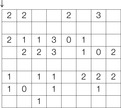 |
1. Model the problem as a satisfiability problem.
2. Solve the problem using an SAT solver.
13.5
1. Solve the problems in Figure 13.2 by using a CSP solver.
2. Generate Sudokus automatically. One frequently used method is to first start with a filled Sudoku, then transpose some rows and columns, and then remove numbers without affecting the uniqueness of the solution.
3. Illustrate how to use CSP technology to provide hints for a human to solve Sudokus.
13.6
1. Formalize the Bipartite Matching problem between a set of n males and f females as a CSP.
2. Suppose we have m male and f females (of  persons) to be grouped together and set up a basket experiment, with names on the balls. Now we draw two balls, one after the other, without putting one back. Determine m and f dependent on n so that the probability that the sexes for the first and second ball are different is 1/2. For example n = 4, we have m = 1 and f = 3, since the probability
  of drawing first a male then a female and equal to the probability
  of drawing first a female then a male. You may assume n to be a square number and f > m.
13.7 The k-Graph Coloring asks for a mapping from the set of nodes to the set of k colors, so that no two adjacent nodes share the same color.
1. Show that deciding 2-Graph Coloringing can be decided in polynomial time.
2. Show that 3-Graph Coloringing is NP-hard.
3. Formalize the 3-coloring problem as a CSP.
4. Show that the graph with edges (1,2), (1,3), (2,3), (2,4), (3,4), (4,5), (5,6), (3,5), (3,6) can be 3-colored by providing mapping to the color set {1,2,3}.
13.8 The n-Queens problem aims at placing n nonconflicting queens on a chess board of size  . Write a recursive backtracking search program to generate a feasible solution. To ease the search, use an array representing the queen positions in each row. How big can you raise n until CPU time exceeds one hour?
Show that for the n-Queens problem, there is no need to search at all. Take the board to be enumerated from 1 to n along both coordinate axes. We define a knight pattern S at  to be the set of squares a knight can reach using an up-right jump:
 .
.
1. Show that for all even n in  the pattern
  is a solution to n-Queens. For n = 6 we have:
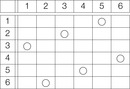 |
2. Show that for an uneven n in  we can derive an almost identical solution. An example for n = 7 is as follows:
 |
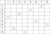
4. Prove that the pattern for odd n in  can be found by an extension of
  followed by an enlargement of
  at column
  . An example for
  is as follows:
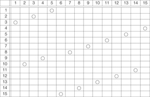 |
1. Show that the constraint is not bounds consistent with D.
2. Find domains for X, Y, and Z that are bounds consistent.
13.11 Determine the propagation rules for the constraint  .
.
1. Rewrite the expression into three forms, one for each variable.
2. Obtain inequalities based on minD and maxD.
3. Test the rules with the initial domain  .
.
13.12 A Knapsack has limited weight capacity of 9 units. Product 1 has weight 4, product 2 has weight 3, and product 3 has weight 2. The profits for products are 15 units, 10 units, and 7 units, respectively. Determine the selection of products for the Knapsack to obtain a profit of 20 units or more.
1. Specify the CSP corresponding to the problem.
2. Apply bounds consistency to the initial domains  .
.
3. For the labeling choose branch X = 0 first and apply bounds consistency once more.
4. Now choose branch Y = 1 and apply bounds consistency to obtain a solution to the problem. What is the value of Z?
5. Determine all alternative solutions to the problem.
13.13 Display the selection of the first three paths in a complete binary tree of height 5 with
1. Linear discrepancy search.
2. Improved LDS.
3. Depth-bounded LDS.
13.14 Show that original LDS generates a total of 19 different paths for a depth-three binary tree, only eight of which are unique.
13.15 To compute the time efficiency of LDS we have to count all internal nodes that are generated. We assume a complete b-ary search tree to a uniform depth d.
1. Show that the total number of nodes generated by improved LDS is the same as the number of nodes generated by depth-first iterative-deepening search.
2. Use your result to prove that the total number of nodes generated by improved LDS is approximated by  .
.
13.16 Consider the following sequential schedule:
 |
The action is prefixed by its starting time while the duration of the action is shown in brackets. The precedence relation includes conflicts between flying (zooming) and boarding (debarking, refueling). Refueling, boarding, and debarking actions can be carried out concurrently, while flying and zooming can obviously not.
1. Use PERT scheduling to compute an optimal parallel plan. When do the actions start and end in the schedule?
2. Model and solve the problem using simple temporal networks.
13.17 Partition the numbers 2, 4, 5, 9, 10, 12, 13, and 16 into two sets.
1. Compute the greedy heuristic for it.
2. Compute the KK heuristic for it.
3. Apply CKKA to find a solution to the problem; that is, draw the search tree.
13.18 Show that the running time for Number Partition with the DAC strategy of Horowitz and Sahni can be improved to time  by a refined sorting strategy.
13.19 For a problem L and a polynomial p let Lp be the subproblem in which only inputs with  are allowed, where
  is the largest value in the input w. A problem L is NP-complete in the strong sense, if Lp is NP-complete. Show
1. Number Partition is not complete in the strong sense.
2. TSP is NP-complete in the strong sense.
13.20 With the refined methods for Rectangle Packing it is possible to pack the 1 × 1, …,  squares into a
  square. Verify that the minimum area that must be left is 49 units.
13.21 A related problem attributed to Golumb is the task to find the Smallest Enclosing Square: For each set of squares from 1 × 1 to  , what is the smallest square that can contain them all? By the search based on wasted space validate the following table. How far can you scale?
13.22 Show that Simple Max Cut can be reduced from 3-SAT.
1. Show that MAX-2-SAT can be reduced from 3-SAT.
2. Show that Simple Max Cut can be reduced from MAX-2-SAT.
13.23 Improve heuristic h1 in Graph Partition by drawing inferences on the free graph that connects free vertices in A′ and in B′.
1. Provide a number N(x) of allowed edges for x i.e., Type 3 edges that will be added to h1 if we move x from one component to another.
2. Take as many edges as possible from the free graph and form a subgraph such that no node x will be connected to more than N(x) neighbors. Solve the induced generalized matching problem using network flow efficiently.
3. The computed flow F finally yields the heuristic  . Show that the heuristic is admissible.
13.24 The research in Satisfiability has influenced the interest in more flexible formula specifications. The problem Quantified Boolean Formula (QBF-SAT) asks if formulas of the form  with
with  are satisfiable.
1. Show that 2-QBF-SAT is in P by extending the algorithm for 2-SAT.
2. Show that QBF-SAT is PSPACE-complete.
1. For showing QBF-SAT in DTAPE , use that
  and
and  can be merged to the overall evaluation
  on constant space.
2. Show that for all L in PSPACE,  can be polynomially reduced to L. If ML is a deterministic Turing machine, bounded to p(n) space and
  time, for input x, construct a QBF formula Qx of size
  , which is satisfied if and only if ML accepts x. Avoid recursion in both subformulas.
13.25
1. Show that if LTL-Solve terminates at a node u with  , no successor of u will ever fulfill the imposed path constraint.
2. Extend the pseudo code to add formula progression to A*.
13.26 Generalize the result of bounded arithmetic constraints  to b-bit variables
  .
.
1. Explain the working of Algorithm 13.20 by constructing the BDD for  for 4-bit values. The algorithm is initially invoked by calling Node
  .
.
2. Consider the conjunction/disjunction of several linear arithmetic formulas of the form  . Show that the satisfiability of a conjunction of m linear constraints can be solved in time
  .
.
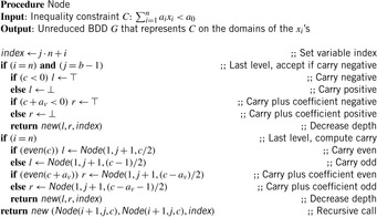
13.11. Bibliographic Notes
There are many introductory books to CSP solving and programming, like the ones by Mariott and Stuckey (1998), Hentenryck (1989), Tsang (1993), or Rossi et al. (2006). Most of the problems are very well related to other discussions in the book (e.g., automated planning) and include search heuristics. A surveying online guide to constraint programming is maintained by Roman Bartàk.
The complexity of cryptarithms has been discussed by Eppstein (1987). Sudoku (Su translates to number, doku translates to single(ton)) most likely was introduced in the 1970s. Under the name Kaji Maki it appeared in the journal Monthly Nikolist in 1984.
AC-3 is due to Mackworth (1977). There have been several improvements that have been proposed to enhance the traversal in AC-3/AC-8. For example, AC-4 by Mohr and Henderson (1986) computes the sets of supporting values in optimal worst-case time, and AC-5 by Hentenryck et al. (1992) covers both AC-4 and AC-3. The algorithm AC-6 by Bessiere (1994) further improves AC-4 by remembering just one supporting value for a variable, and AC-7 by Bessiere et al. (1999) improves AC-6 by exploiting symmetries that are constraints. AC-2000 by Bessiere and Regin (2001) is an adaptive version of AC-3 that either looks for support or propagates deletions; AC-2001 by Bessiere and Regin (2001) and AC-3.1 by Zhang and Yap (2001) are recent improvements of AC-3 to achieve optimality.
The path consistency algorithm presented in the text is also due to Mackworth (1977). He revised it to PC-2 to revise only a subset of relevant paths. Mohr and Henderson (1986) have extended PC-2 to PC-3 based on AC-4, but the extension was unsound, and could delete a consistent value. A correct version of PC-3, denoted as PC-4, has been proposed by Han and Lee (1988). The version PC-5 by Singh (1995) is based on principles of AC-6. The all-different constraint based on matching theory has been presented by Regin (1994).
As search refinements to chronological backtracking that upon failure backtrack to the penultimate variable, backjumping by Gaschnig (1979c) jumps back to a conflicting one. Dynamic backtracking by Ginsberg (1993) upon failure unassigns only the conflicting variable and backmarking by Haralick and Elliot (1980) remembers no-goods and uses them in subsequent searches.
Not all algorithms that have been tested are complete; for example, bounded backtrack search by Harvey (1995) restricts the number of backtracks and depth-bounded backtrack search by Cheadle et al. (2003) restricts the depth where alternatives are explored. In iterative broadening by Ginsberg and Harvey (1992) we have a restricted number of successors (breadth) in each node. Credit search by Cheadle et al. (2003) is a more recent technique that computes limited credit for exploring alternatives and splits among the alternatives.
The linear discrepancy search scheme has been invented by Harvey and Ginsberg (1995) and later was improved by Korf (1996). Depth-bounded discrepancy search is due to Walsh (1997). A related strategy, called interleaved depth-first search, has been contributed by Meseguer (1997). It searches depth-first several so-called active subtrees in parallel, and assumes a single processor on which it interleaves DFS on active subtrees.
The book by Dechter (2004) includes an introduction to temporal networks and their application. The theorem on the minimal temporal networks is due to Shostak (1981) and to Leiserson and Saxe (1983). The application of PERT to scheduling of partial or completed temporal plans for a heuristic search solver has been proposed by Edelkamp (2003c). A related approach based on simple temporal networks is due to Coles et al. (2009).
The theory of NP-completeness was initiated by the theorem of Cook (1971), who has shown that the satisfiability problem SAT is NP-complete by devising a polynomial encoding of the computations of a nondeterministic Turing machine with SAT clauses. Garey and Johnson (1979) have enlarged the theory of NP-completeness to a wide range of problems. Some results refer to joint work by Garey et al. (1974).
The problem of phase transition goes back to early work of Erdös and Renyi of analyzing thresholds in random graphs. The research of phase transition in AI was initiated by Cheeseman et al. (2001). For the phase transition parameter (for the ratio between the number of clauses and the number of variables) in 3-SAT, lower bounds of  , and upper bounds of
  have been shown. Backbones are studied by Slaney and Walsh (2001). In Zhang (2004b) the connection of backbones and phase transition in 3-SAT problems is discussed. Their effect on local search algorithms has been considered by Zhang (2004a). The hardness of backbones have been addressed Beacham (2000). Backdoors have been reported in Ruan et al. (2004). The algorithms to compute strong and weak backdoors have been provided by Kilby et al. (2005).
Aspvall et al. (1979) showed that 2-SAT and 2-QBF-SAT are in P. Many good SAT solvers in practice refer to Chaff by Moskewicz et al. (2001). Some of the refinements discussed for the DPLL algorithm refer to this implementation. Branch-and-bound has been applied to MAX-SAT by Hsu and McIlraith (2010) and hill-climbing search with gradients to MAX-k-SAT by Sutton et al. (2010).
Karmarkar and Karp (1982) have devised the polynomial-time approximation algorithm for Number Partition. Later, the conjecture that the value of the final difference in the KK heuristic is of order  for some constant c was confirmed. Horowitz and Sahni (1974) have shown how to reduce the trivial 2n algorithm. Schroeppel and Shamir (1981) have improved the algorithm by reducing the space complexity from
  to
to  , without increasing the runtime complexity. In the Shroepel and Shamir algorithm, the subsets are generated on demand maintaining subset sums on four equal-sized subsets. Korf (1998) has extended this approximation to the complete (anytime) algorithm. The extension of the 2- to k-Number Partitioning problem (Multiway Number Partition) has been studied by Korf (2009), with an approach that has been corrected in Korf (2010). The importance of this problem for scheduling where numbers are the time it takes for k-equal processors to process a job and the goal is to minimize the makespan, is obvious.
Optimal Bin Packing has been considered by Korf (2002) in the bin completion algorithm with lower bounds for the bin packing problem that has been proposed by Martello and Toth (1990). An improved algorithm based on a faster algorithm to generate all undominated completions of a bin and a better pruning has been presented by Korf (2003b).
Most work on Rectangle Packing deals with approximate rather than optimal solutions. However, in resource constraint scheduling problems and in the design of VLSI chips, where rectangle packing is applied, deriving optimal solutions is of practical interest. Initial results on optimal Rectangle Packing have been given by Korf (2003c), with new results provided in the work by Korf (2004b). The work refers to an article of Gardner (1966). Comparable good results have been achieved by Moffitt and Pollack (2006) who avoid discretization of the rectangles. According to Gardner (1966) smallest enclosing square problem has been solved by Golumb, Conway, and Reid for n up to 17.
Solving Clique problems with state space search methods has been considered by Stern et al. (2010a). Surprisingly good approximate results to vertex cover have been presented by Richter et al. (2007). There is increasing interest in the Canadian Traveler's Problem with promising results, for example, the ones given by Eyerich et al. (2010) and by Bnaya et al. (2009).
Another challenge for heuristic search in constraint processing is the computation of the tree width for the bucket elimination algorithm of Dechter (1999). It is determined by the maximum degree in any elimination order of variables. States are too large in main memory, and reconstruction schemes apply Dow and Korf (2007). Zhou and Hansen (2008) have proposed a combination of depth-first and breadth-first search.
Applying temporal logics to constrain the search is a widespread field. There are two concurrent approaches: formula progression as applied, for example, by Bacchus and Kabanza (2000); and automata as applied in model checking, for example, by Wolper (1983). Which one turns out to be the more efficient overall approach is yet unresolved, but there is some initial data by Kerjean et al. (2005) on comparing the two approaches in the context of analyzing plan synthesis problems.
Path constraints provide an important step toward the description of temporal control knowledge by Bacchus and Kabanza (2000) and temporally extended goals by DeGiacomo and Vardi (1999). To take care of both extended goals and control knowledge, Kabanza and Thiebaux (2005) have applied a hybrid algorithm, formula progression for the control knowledge, and Büchi automata for analyzing the temporally extended goal. The methods are applied concurrently for an extended state vector that includes currently progressed formula and the current state in the Büchi automaton.
Many planners support search control knowledge like TALPlan Kvarnström et al. (2000) or TLPlan by Bacchus and Kabanza (2000), while planners for temporally extended goals like MBP (see Lago et al. (2002); Pistore and Traverso (2001)) often do not incorporate heuristic search. Progress on heuristic search model checking for temporally extended goals has been documented by Baier and McIlraith (2006) and Edelkamp (2006). The first one uses derived predicates to compile the properties into, and the second approach applies automata theory to compile the temporally extended goals away, as illustrated here. Rintanen (2000) has compared formula progression as in TLPlan with a direct translation into plan operators. His translation applies all changes to the operators so that produced plans remain unchanged. Instead of PDDL input, he has considered a set of clauses with next-time and until. Fox et al. (2004) have considered the transformation of maintenance and deadline goals in the context of PDDL2 planning. The setting is slightly different as they consider formulas of the type Up c (and Fp c), where p is the condition until which (or from which) condition c must hold.
Although soft constraints have been extensively studied in the CSP literature, only recently has the search community started to investigate them; see, for example, Brafman and Chernyavsky (2005), Smith (2004) and Briel et al. (2004). More recently, plan and preference constraints have been integrated into PDDL, the description language for problems in action planning Gerevini and Long (2005). Baier (2009) has tackled planning with soft constraints on temporally extended goals. A set of new heuristics and another search algorithm have been proposed to guide the planner toward preferred plans.
The work of Bartzis and Bultan (2006) has been studied to the efficiency of BDD for bounded arithmetic constraints. The authors have also illustrated how to handle multiplication, overflows, and multiple bounds. The experimental results were impressive, since the approach could solve appropriate model checking problems orders of magnitudes faster than previous state-of-the-art approaches.
..................Content has been hidden....................
You can't read the all page of ebook, please click here login for view all page.