
Chapter 8. External Search
This chapter studies the integration of disk space into the search, trying to minimize the number of block accesses. It introduces the theory of external memory algorithms and studies disk-based search with the delayed detection of duplicates and its variants.
Keywords: virtual memory, external scanning, external sorting, external priority queue, external explicit graph depth-first search, external explicit graph breadth-first search, delayed duplicate detection, external breadth-first branch-and-bound, external enforced hill-climbing, external A*, hash-based duplicate detection, structured duplicate detection, pipelining, external iterative-deepening search, external pattern databases, external value iteration, flash-memory search
Often search spaces are so large that even in compressed form they fail to fit into the main memory. During the execution of a search algorithm, only a part of the graph can be processed in the main memory at a time; the remainder is stored on a disk.
It has been observed that the law of Intel cofounder Gordon Moore moves toward external devices. His prediction, popularly known as Moore's Law, states that the number of transistors on a chip doubles about every two years. The costs for large amounts of disk space have decreased considerably. But hard disk operations are about  to
to  times slower than main memory accesses and technological progress yields annual rates of about 40% increase in processor speeds, while disk transfers improve only by about 10%. This growing disparity has led to a growing attention to the design of I/O-efficient algorithms in recent years.
Most modern operating systems hide secondary memory accesses from the programmer, but offer one consistent address space of virtual memory that can be larger than internal memory. When the program is executed, virtual addresses are translated into physical addresses. Only those portions of the program currently needed for the execution are copied into main memory. Caching and prefetching heuristics have been developed to reduce the number of page faults (the referenced page does not reside in the cache and has to be loaded from a higher memory level). By their nature, however, these methods cannot always take full advantage of the locality inherent in algorithms. Algorithms that explicitly manage the memory hierarchy can lead to substantial speedups, since they are more informed to predict and adjust future memory access.
We first give an introduction to the more general topic of I/O-efficient algorithms. We introduce the most widely used computation model, which counts inputs/outputs (I/Os) in terms of block transfers of fixed-size records to and from secondary memory. As external memory algorithms often run for weeks and months, a fault-tolerant hardware architecture is needed and discussed in the text. We describe some basic external memory algorithms like scanning and sorting, and introduce data structures relevant to graph search.
Then we turn to the subject of external memory graph search. In this part we are mostly concerned with breadth-first and Single-Source Shortest Path search algorithms that deal with graphs stored on disk, but we also provide insights on external (memory) depth-first search. The complexity for the general case is improved by exploiting properties of certain graph classes.
For state space search, we adapt external breadth-first search to implicit graphs. As the use of early duplicate pruning in a hash table is limited, in external memory search the pruning concept has been coined to the term delayed duplicate detection for frontier search. The fact that no external access to the adjacency list is needed reduces the I/O complexity to the minimum possible.
External breadth-first branch-and-bound conducts a cost-bounded traversal of the state space for more general cost functions. Another impact of external breadth-first search is that it serves as a subroutine in external enforced hill-climbing. Next, we show how external breadth-first search can be extended to feature A*. As external A* operates on sets of states, it shares similarities with the symbolic implementation of A*, introduced in Chapter 7.
We discuss different sorts of implementation refinements; for example, we improve the I/O complexity for regular graphs and create external pattern databases to compute better search heuristics. Lastly, we turn to the external memory algorithm for nondeterministic and probabilistic search spaces. With external value iteration we provide a general solution for solving Markov decision process problems on disk.
8.1. Virtual Memory Management
Modern operating systems provide a general-purpose mechanism for processing data larger than available main memory called virtual memory. Transparent to the program, swapping moves parts of the data back and forth from disk as needed. Usually, the virtual address space is divided into units calledpages; the corresponding equal-size units in physical memory are called page frames. A page table maps the virtual addresses on the page frames and keeps track of their status (loaded/absent). When a page fault occurs (i.e., a program tries to use an unmapped page), the CPU is interrupted; the operating system picks a rarely picked page frame and writes its contents back to the disk. It then fetches the referenced page into the page frame just freed, changes the map, and restarts the trapped instruction. In modern computers memory management is implemented on hardware with a page size commonly fixed at 4,096 bytes.
Various paging strategies have been explored that aim at minimizing page faults. Belady has shown that an optimal offline page exchange strategy deletes the page that will not be used for a long time. Unfortunately, the system, unlike possibly the application program itself, cannot know this in advance. Several different online algorithms for the paging problem have been proposed, such as last-in-first-out (LIFO), first-in-first-out (FIFO), least-recently-used (LRU), and least-frequently-used (LFU). Despite that Sleator and Tarjan proved that LRU is the best general online algorithm for the problem, we reduce the number of page faults by designing data structures that exhibit memory locality, such that successive operations tend to access nearby memory cells.
Sometimes it is even desirable to have explicit control of secondary memory manipulations. For example, fetching data structures larger than the system page size may require multiple disk operations. A file buffer can be regarded as a kind of software paging that mimics swapping on a coarser level of granularity. Generally, an application can outperform the operating system's memory management because it is well informed to predict future memory access.
Particularly for search algorithms, system paging often becomes the major bottleneck. This problem has been experienced when applying A* to the domain of route planning. Moreover, A* does not respect memory locality at all; it explores nodes in the strict order of f-values, regardless of their neighborhood, and hence jumps back and forth in a spatially unrelated way.
8.2. Fault Tolerance
External algorithms often run for a long time and have to be robust with respect to the reliability of existing hardware. Unrecoverable error rates on hard disks happen at a level of about 1 in  bits. If such an error occurs in critical system areas, the entire file system is corrupted. In conventional usage, such errors happen every 10 years. However, in extensive usage with file I/O in the order of terabytes per second, such a worst-case scenario may happen every week. As one solution to the problem, a redundant array of inexpensive disks (RAID) 1 is appropriate. Some of its levels are: 0 (striping: efficiency improvement for the exploration due to multiple disk access without introducing redundancy); 1 (mirroring: reliability improvement for the search due to option of recovering data); and 5 (performance and parity: reliability and efficiency improvement for the search, automatically recovers from one-bit disk failures).
Another problem with long-term experiments are environmental faults that lead to switched-down power supply. Even if data is stored on disk, it is not certain that all data remains accessible in case of a failure. As hard disks may have individual reading and writing buffers, disk access is probably not under full control by the application program or the operating system. Therefore, it can happen that a file is deleted when the file reading buffer is still unprocessed. One solution to this problem is uninteruptable power supplies (UPSs) that assist in writing volatile data to disk. In many cases like external breadth-first search it continues the search from some certified flush like the last layer fully expanded.
8.3. Model of Computation
Recent developments of hardware significantly deviate from the von Neumann architecture; for example, the next generation of processors has multicore processors and several processor cache levels (see Fig. 8.1). Consequences like cache anomalies are well known; for example, recursive programs like Quicksort perform unexpectedly well in practice when compared to other theoretically stronger sorting algorithms.

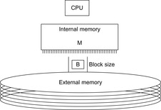
The commonly used model for comparing the performances of external algorithms consists of a single processor, small internal memory that can hold up to M data items, and unlimited secondary memory. The size of the input problem (in terms of the number of records) is abbreviated by N. Moreover, the block size B governs the bandwidth of memory transfers. It is often convenient to refer to these parameters in terms of blocks, so we define  and
and  . It is usually assumed that at the beginning of the algorithm, the input data is stored in contiguous blocks on external memory, and the same must hold for the output. Only the number of block read and writes are counted, and computations in internal memory do not incur any cost (see Fig. 8.2). An extension of the model considers D disks that can be accessed simultaneously. When using disks in parallel, the technique of disk striping can be employed to essentially increase the block size by a factor of D. Successive blocks are distributed across different disks. Formally, this means that if we enumerate the records from zero, the i th block of the j th disk contains record number
  through
  . Usually, it is assumed that
  and
and  .
.
We distinguish two general approaches of external memory algorithms: either we can devise algorithms to solve specific computational problems while explicitly controlling secondary memory access, or we can develop general-purpose external memory data structures, such as stacks, queues, search trees, priority queues, and so on, and then use them in algorithms that are similar to their internal memory counterparts.
8.4. Basic Primitives
It is often convenient to express the complexity of external memory algorithms using two frequently occurring primitive operations. These primitives, together with their complexities, are summarized in Table 8.1. The simplest operation is external scanning, which means reading a stream of records stored consecutively on secondary memory. In this case, it is trivial to exploit disk and block parallelism. The number of I/Os is  .
.
Sorting is a fundamental problem that arises in almost all areas of computer science. For the heuristic search exploration, sorting is essential to arrange similar states together, for example, to find duplicates. For this purpose, sorting is useful to eliminate I/O accesses. The proposed external sorting algorithms fall into two categories: those based on the merging paradigm, and those based on the distribution paradigm.
| Operation | Complexity | Optimality Achieved By |
|---|---|---|
| Trivial sequential access | ||
| merge or distribution sort |
External Mergesort converts the input into a number of elementary sorted sequences of length M using internal memory sorting. Subsequently, a merging step is applied repeatedly until only one run remains. A set of k sequences  can be merged into one run with
  I/O operations by reading each sequence in a blockwise manner. In internal memory, k cursors
  are maintained for each of the sequences; moreover, it contains one buffer block for each run, and one output buffer. Among the elements pointed to by the
  , the one with the smallest key, say
  , is selected; the element is copied to the output buffer, and
  is incremented. Whenever the output buffer reaches the block size B, it is written to disk and emptied; similarly, whenever a cached block for an input sequence has been fully read, it is replaced with the next block of the run in external memory. When using one internal buffer block per sequence and one output buffer, each merging phase uses
  operations. The best result is achieved when k is chosen as big as possible,
  . Then sorting can be accomplished in
  phases, resulting in the overall optimal complexity.
On the other hand, External Quicksort partitions the input data into disjoint sets  ,
,  , such that the key of each element in
  is smaller than that of any element in
  , if
, if  . To produce this partition, a set of splitters
  is chosen, and
  is defined to be the subset of elements
  with
with  . The splitting can be done I/O-efficiently by streaming the input data through an input buffer, and using an output buffer. Then each subset
  is recursively processed, unless its size allows sorting in internal memory. The final output is produced by concatenating all the elementary sorted subsequences. Optimality can be achieved by a good choice of splitters, such that
  . It has been proposed to calculate the splitters in linear time based on the classic internal memory selection algorithm to find the k-smallest element. We note that although we will be concerned only with the case of a single disk (
 ), it is possible to make optimal use of multiple disks with
 I/Os. Simple disk striping, however, does not lead to optimal external sorting. It has to be ensured that each read operation brings in
  blocks, and each write operation must store
  blocks on disk. For External Quicksort, the buckets have to be hashed to the disks almost uniformly. This can be achieved using a randomized scheme.
8.5. External Explicit Graph Search
External explicit graphs are problem graphs that are stored on disk. Examples are large maps for route planning systems. Under external explicit graph search, we understand search algorithms that operate in explicitly specified directed or undirected graphs that are too large to fit in main memory. We distinguish between assigning BFS or DFS numbers to nodes, assigning BFS levels to nodes, or computing the BFS or DFS tree edges. However, for BFS in undirected graphs it can be shown that all these formulations are reducible to each other in  I/Os, where V and E are the sets of nodes and edges of the input graph (see Exercises).
The input graph consists of two arrays, one that contains all edges sorted by the start node, and one array of size  that stores, for each vertex, its out-degree and offset into the first array.
8.5.1. *External Priority Queues
External priority queues for general weights are involved. An I/O-efficient algorithm for the Single-Source Shortest Paths problem simulates Dijkstra's algorithm by replacing the priority queue with the Tournament Tree data structure. It is a priority queue data structure that was developed with the application to graph search algorithms in mind; it is similar to an external heap, but it holds additional information. The tree stores pairs  , where
  identifies the element, and y is called the key. The Tournament Tree is a complete binary tree, except for possibly some right-most leaves missing. It has
  leaves. There is a fixed mapping of elements to the leaves, namely, IDs in the range from
  through the
  map to the i th leaf. Each element occurs exactly once in the tree. Each node has an associated list of
  to M elements, which are the smallest ones among all descendants. Additionally, it has an associated buffer of size M. Using an amortization argument, it can be shown that a sequence of k Update, Delete, or DeleteMin operations on a tournament tree containing N elements requires at most
  accesses to external memory.
The Buffered Repository Tree is a variant of the Tournament Tree that provides two operations: Insert  inserts element x under key y, where several elements can have the same key. ExtractAll
  returns and removes all elements that have key y. As in a Tournament Tree, keys come from a key set
  , and the leaves in the static height-balanced binary tree are associated with the key ranges in the same fixed way. Each internal node stores elements in a buffer of size B, which is recursively distributed to its two children when it becomes full. Thus, an Insert operation needs
  I/O amortized operations. An ExtractAll operation requires
  accesses to secondary memory, where the first term corresponds to reading all buffers on the path from the root to the correct leaf, and the second term reflects reading the x reported elements from the leaf. Moreover, a Buffered Repository Tree T is used to remember nodes that were encountered earlier. When v is extracted, each incoming edge
  is inserted into T under key u. If at some later point u is extracted, then ExtractAll
  on T yields a list of edges that should not be traversed because they would lead to duplicates. The algorithm takes
  I/Os to access adjacency lists. The
  operations on the priority queues take at most
  times, leading to a cost of
  . Additionally, there are
  Insert and
  ExtractAll operations on T, which add up to
  I/Os; this term also dominates the overall complexity of the algorithm.
More efficient algorithms can be developed by exploiting properties of particular classes of graphs. In the case of directed acyclic graphs (DAGs) like those induced in Multiple Sequence Alignment problems, we can solve the shortest path problem following a topological ordering, in which for each edge  the index of u is smaller than that of v. The start node has index 0. Nodes are processed in this order. Due to the fixed ordering, we can access all adjacency lists in
  time. Since this procedure involves
  priority queue operations, the overall complexity is
  .
.
It has been shown that the Single-Source Shortest Paths problem can be solved with  I/Os for many subclasses of sparse graphs; for example, for planar graphs that can be drawn in a plane in the natural way without having edges cross between nodes. Such graphs naturally decompose the plane into faces. For example, route planning graphs without bridges and tunnels are planar. As most special cases are local, virtual intersections may be inserted to exploit planarity.
We next consider external DFS and BFS exploration for more general graph classes.
8.5.2. External Explicit Graph Depth-First Search
External DFS relies on an external stack data structure. The search stack is often small compared to the overall search but in the worst-case scenario it can become large. For an external stack, the buffer is just an internal memory array of 2B elements that at any time contains the  elements most recently inserted. We assume that the stack content is bounded by at most N elements. A pop operation incurs no I/O, except for the case when the buffer has run empty, where
  I/O to retrieve a block of B elements is sufficient. A push operation incurs no I/O, except for the case the buffer has run full, where
  I/O is needed to retrieve a block of B elements. Insertion and deletion take
  I/Os in the amortized sense.
The I/O complexity for external DFS for explicit (possibly directed) graphs is  . There are
  phases where the internal buffer for the visited state set becomes full, in which case it is flushed. Duplicates are eliminated not via sorting (as in the case of external BFS) but by removing marked states from the external adjacency list representation by a file scan. This is possible as the adjacency is explicitly represented on disk and done by generating a simplified copy of the graph and writing it to disk. Successors in the unexplored adjacency lists that are visited are marked not to be generated again, such that all states in the internal visited list can be eliminated. As with external BFS in explicit graphs,
  I/Os are due to the unstructured access to the external adjacency list. Computing strongly connected components in explicit graphs also takes
  I/Os.
I/Os.
Dropping the term of  I/O as with external BFS, however, is a challenge. For implicit graphs, no access to an external adjacency list is possible, so that we cannot access the search graph that has not been seen so far. Therefore, the major problem for external DFS exploration in implicit graphs is that adjacencies defining the successor relation cannot be filtered out as done for explicit graphs.
8.5.3. External Explicit Graph Breadth-First Search
Recall the standard internal memory BFS algorithm, visiting each reachable node of the input problem graph G one by one utilizing a FIFO queue. After a node is extracted, its adjacency list (the sets of successors in G) is examined, and those that haven't been visited so far are inserted into the queue in turn. Naively running the standard internal BFS algorithm in the same way in external memory will result in  I/Os for unstructured accesses to the adjacency lists, and
  I/Os to check if successor nodes have already been visited. The latter task is considerably easier for undirected graphs, since duplicates are constrained to be located in adjacent levels.
The algorithm of Munagala and Ranade improves I/O complexity for the case of undirected graphs, in which duplicates are constrained to be located in adjacent levels.
The algorithm builds  from
from  as follows: Let
  be the multiset of successors of nodes in
  ;
;  is created by concatenating all adjacency lists of nodes in
  . Then the algorithm removes duplicates by external sorting followed by an external scan. Since the resulting list
  is still sorted, filtering out the nodes already contained in the sorted lists
  or
or  is possible by parallel scanning. This completes the generation of
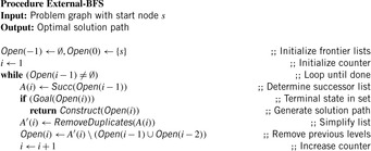
  . Set U maintains all unvisited nodes necessary to be looked at when the graph is not completely connected. Algorithm 8.1 provides the implementation of the algorithm of Munagala and Ranade in pseudo code. The algorithm can record the nodes' BFS level in additional
  time using an external array.

Theorem 8.1
(Efficiency Explicit Graph External BFS) On an undirected explicit problem graph, the algorithm of Munagala and Ranade requires at most  I/Os to compute the BFS level for each state.
Proof
For the correctness argument, we assume that the state levels  have already been assigned to the correct BFS level. Now we consider a successor v of a node
  : The distance from s to v is at least
  because otherwise the distance of u would be less than
  . Thus,
  . Therefore, we can correctly assign
  to
to  .
.
For the complexity argument we assume that after preprocessing, the graph is stored in adjacency-list representation. Hence, successor generation takes  I/Os. Duplicate elimination within the successor set takes
  I/Os. Parallel scanning can be done using
  I/Os. Since
  and
and  , the execution of external BFS requires
  time, where
  is due to the external representation of the graph and the initial reconfiguration time to enable efficient successor generation.
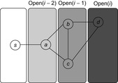
An example is provided in Figure 8.3. When generating  we unify
  with
with  . Removing the duplicates in
  yields set
  . Removing
  reduces the set to
  ; omitting
  results in the final node set
  .
.
The bottleneck of the algorithm are the  unstructured accesses to adjacency lists. The following refinement of Mehlhorn and Meyer consists of a preprocessing and a BFS phase, arriving at a complexity of
  I/Os.
I/Os.
The preprocessing phase partitions the graph into K disjoint subgraphs  with small internal shortest path distances; the adjacency lists are accordingly partitioned into consecutively stored sets
  as well. The partitions are created by choosing seed nodes independently with uniform probability
  . Then K BFS are run in parallel, starting from the seed nodes, until all nodes of the graph have been assigned to a subgraph. In each round, the active adjacency lists of nodes lying on the boundary of their partition are scanned; the requested destination nodes are labeled with the partition identifier, and are sorted (ties between partitions are arbitrarily broken). Then, a parallel scan of the sorted requests and the graph representation can extract the unvisited part of the graph, as well as label the new boundary nodes and generate the active adjacency lists for the next round. The expected I/O bound for the graph partitioning is
  ; the expected shortest path distance between any two nodes within a subgraph is
  . The main idea of the second phase is to replace the nodewise access to adjacency lists by a scanning operation on a file H that contains all
  in sorted order such that the current BFS level has at least one node in
  . All subgraph adjacency lists in
  are merged with H completely, not node by node. Since the shortest path within a partition is of order
  , each
  stays in H accordingly for at most
  levels. The second phase uses
  I/Os in total; choosing
  , we arrive at a complexity of
  I/Os. An alternative to the randomized strategy of generating the partition described here is a deterministic variant using a Euler tour around a minimum spanning tree. Thus, the bound also holds in the worst case.
8.6. External Implicit Graph Search
An implicit graph is a graph that is not residing on disk but generated by successively applying a set of actions to nodes selected from the search frontier. The advantage in implicit search is that the graph is generated by a set of rules, and hence no disk accesses for the adjacency lists are required.
Considering the I/O complexities, bounds like those that include  are rather misleading, since we are often trying to avoid generating all nodes. Hence, value
  is needed only to derive worst-case bounds. In almost all cases,
  can safely be substituted by the number of expanded nodes.
8.6.1. Delayed Duplicate Detection for BFS
A variant of Munagala and Ranade's algorithm for BFS in implicit graphs has been coined with the term delayed duplicate detection for frontier search. Let s be the initial node, and  be the implicit successor generation function. The algorithm maintains BFS layers on disk. Layer
  is scanned and the set of successors are put into a buffer of a size close to the main memory capacity. If the buffer becomes full, internal sorting followed by a duplicate elimination phase generates a sorted duplicate-free node sequence in the buffer that is flushed to disk. The outcome of this phase are k presorted files. Note that delayed internal duplicate elimination can be improved by using hash tables for the blocks before being flushed to disk. Since the node set in the hash table has to be stored anyway, the savings by early duplicate detection are often small.
In the next step, external merging is applied to unify the files into  by a simultaneous scan. The size of the output files is chosen such that a single pass suffices. Duplicates are eliminated. Since the files were presorted, the complexity is given by the scanning time of all files. We also have to eliminate
  and
and  from
from  to avoid recomputations; that is, nodes extracted from the external queue are not immediately deleted, but kept until the layer has been completely generated and sorted, at which point duplicates can be eliminated using a parallel scan. The process is repeated until
  becomes empty, or the goal has been found.
The corresponding pseudo code is shown in Algorithm 8.2. Note that the explicit partition of the set of successors into blocks is implicit. Termination is not shown, but imposes no additional implementation problem.
Theorem 8.2
(Efficiency Implicit External BFS) On an undirected implicit problem graph, external BFS with delayed duplicate elimination requires at most  I/Os.
I/Os.
Proof
The proof for implicit problem graphs is essentially the same for explicit problem graphs with the exception that the access to the external device for generating the successors of a state resulting in at most  I/Os is not needed.
As with the algorithm of Munagala and Ranade, delayed duplicate detection applies  I/Os. As no explicit access to the adjacency list is needed, by
  and
and  , the total execution time is
  I/Os.
I/Os.
In search problems with a bounded branching factor we have  , and thus the complexity for implicit external BFS reduces to
  I/Os. If we keep each
  in a separate file for sparse problem graphs (e.g., simple chains), file opening and closing would accumulate to
  I/Os. The solution for this case is to store the nodes in
  ,
,  , and so forth, consecutively in internal memory. Therefore, I/O is needed, only if a level has at most B nodes.
The algorithm shares similarities with the internal frontier search algorithm (see Ch. 6) that was used for solving the Multiple Sequence Alignment problem. In fact, the implementation has been applied to external memory search with considerable success. The BFS algorithm extends to graphs with bounded locality. For this case and to ease the description of upcoming algorithms, we assume to be given a general file subtraction procedure as implemented in Algorithm 8.3.

In an internal, not memory-restricted setting, a plan is constructed by backtracking from the goal node to the start node. This is facilitated by saving with every node a pointer to its predecessor. For memory-limited frontier search, a divide-and-conquer solution reconstruction is needed for which certain relay layers have to be stored in the main memory. In external search divide-and-conquer solution reconstruction and relay layers are not needed, since the exploration fully resides on disk.
There is one subtle problem: predecessors of the pointers are not available on disk. This is resolved as follows. Plans are reconstructed by saving the predecessor together with every state, by scanning with decreasing depth the stored files, and by looking for matching predecessors. Any reached node that is a predecessor of the current node is its predecessor on an optimal solution path. This results in a I/O complexity that is at most linear to scanning time  .
.
Even if conceptually simpler, there is no need to store the Open list in different files  ,
,  . We may store successive layers appended in one file.
8.6.2. * External Breadth-First Branch-and-Bound
In weighted graphs, external BFS with delayed duplicate detection does not guarantee an optimal solution. A natural extension of BFS is to continue the search when a goal is found and keep on searching until a better goal is found or the search space is exhausted. In searching with nonadmissible heuristics we hardly can prune states with an evaluation larger than the current one. Essentially, we are forced to look at all states. However, if  with monotone heuristic function h we can prune the exploration.
For the domains where cost  is monotonically increasing, external breadth-first branch-and-bound (external BFBnB) with delayed duplicate detection does not prune away any node that is on the optimal solution path and ultimately finds the optimal solution. In Algorithm 8.4, the algorithm is presented in pseudo code. The sets Open denote the BFS layers and the sets A,
  ,
,  are temporary variables to construct the search frontier for the next iteration. States with
  are pruned and states with
  lead to a bound that is updated.
Theorem 8.3
(Cost-Optimality External BFBnB with Delayed Duplicate Detection) For a state space with  , where g denotes the depth and h is a consistent estimate, external BFBnB with delayed duplicate detection terminates with the optimal solution.
Proof
In BFBnB with cost function  , where g is the depth of the search and h a consistent search heuristic, every duplicate node with a smaller depth has been explored with a smaller f-value. This is simple to see as the h-values of the query node and the duplicate node match, and BFS generates a duplicate node with a smaller g-value first. Moreover, u is safely pruned if
  exceeds the current threshold, as an extension of the path to u to a solution will have a larger f-value. Since external BFBnB with delayed duplicate detection expands all nodes u with
  the algorithm terminates with the optimal solution.
Furthermore, we can easily show that if there exists more than one goal node in the state space with a different solution cost, then external BFBnB with delayed duplicate detection will explore less nodes than a complete external BFS with delayed duplicate detection.
Theorem 8.4
(Gain of External BFBnB wrt. External BFS) If  is the number of nodes expanded by external BFBnB with delayed duplicate detection for
  , and
, and  the number of nodes expanded by a complete run of external BFS with delayed duplicate detection, then
  .
.
Proof
External BFBnB does not change the order in which nodes are looked at during a complete external BFS. There can be two cases. In the first case, there exists just one goal node t, which is also the last node in a BFS tree. For this case, clearly  . If there exists more than one goal node in the search tree, let
  be the two goal nodes with
  and
and  . Since
  will be expanded first,
  will be used as the pruning value for all the next iterations. In this case, there does not exist any node u in the search tree between
  and
and  with
with  ,
,  , otherwise
  .
.
Table 8.2 gives an impression of cost-optimal search in a selected optimization problem, reporting the number of nodes in each layer obtained after refinement with respect to the previous layers. An entry in the goal cost column corresponds to the best goal cost found in that layer.
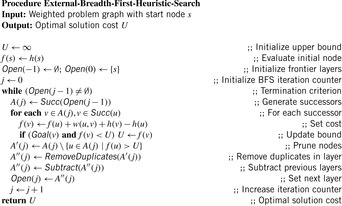
For unit cost search graphs the external branch-and-bound algorithm simplifies to external breadth-first heuristic search (see Ch. 6).
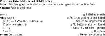
8.6.3. * External Enforced Hill-Climbing
In Chapter 6 we have introduced enforced hill-climbing (a.k.a. iterative improvement) as a more conservative form of hill-climbing search. Starting from a start state, a (breadth-first) search for a successor with a better heuristic value is started. As soon as such a successor is found, the hash tables are cleared and a fresh search is started. The process continues until the goal is reached. Since the algorithm performs a complete search on every state with a strictly better heuristic value, it is guaranteed to find a solution in directed graphs without dead-ends.
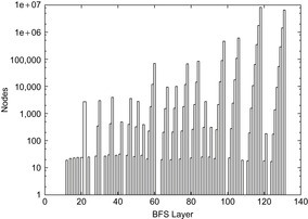
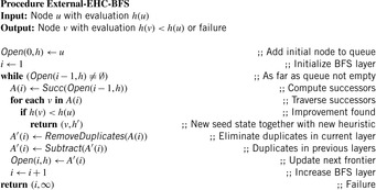
Having external BFS in hand, an external algorithm for enforced hill-climbing can be constructed by utilizing the heuristic estimates. In Algorithm 8.5 we show the algorithm in pseudo-code format. The externalization is embedded in the subprocedure Algorithm 8.6 that performs external BFS for a state that has an improved heuristic estimate. Figure 8.5 shows parts of an exploration for solving a action planning instance. It provides a histogram (logarithmic scale) on the number of nodes in BFS layers for external enforced hill-climbing in a selected planning problem.
Theorem 8.5
(Complexity External Enforced Hill-Climbing) Let  be the heuristic estimate of the initial state. External enforced hill-climbing with delayed duplicate elimination in a problem graph with bounded locality requires at most
  I/Os.
I/Os.
Enforced hill-climbing has one important drawback: its results are not optimal. Moreover, in directed search spaces with unrecognized dead-ends it can be trapped, without finding a solution to a solvable problem.
8.6.4. External A*
In the following we study how to extend external breadth-first exploration in implicit graphs to an A*-like search. If the heuristic is consistent, then on each search path, the evaluation function f is nondecreasing. No successor will have a smaller f-value than the current one. Therefore, the A* algorithm, which traverses the node set in f-order, expands each node at most once. Take, for example, a sliding-tile puzzle. As the Manhattan distance heuristic is consistent, for every two successive nodes u and v the difference of the according estimate evaluations  is either −1 or 1. By the increase in the g-value, the f-values remain either unchanged, or
  .
.
As earlier, external A* maintains the search frontier on disk, possibly partitioned into main memory–size sequences. In fact, the disk files correspond to an external representation of a bucket implementation of a priority queue data structure (see Ch. 3). In the course of the algorithm, each bucket addressed with index i contains all nodes u in the set Open that have priority  . An external representation of this data structure will memorize each bucket in a different file.
We introduce a refinement of the data structure that distinguishes between nodes with different g-values, and designates bucket  to all nodes u with path length
  and heuristic estimate
  . Similar to external BFS, we do not change the identifier Open to separate generated from expanded nodes. In external A* (see Alg. 8.7), bucket
  refers to nodes that are in the current search frontier or belong to the set of expanded nodes. During the exploration process, only nodes from one currently active bucket
  , where
  , are expanded, up to its exhaustion. Buckets are selected in lexicographic order for
  ; then, the buckets
  with
with  and
and  are closed, whereas the buckets
  with
with  or with
  and
and  are open. Depending on the actual node expansion progress, nodes in the active bucket are either open or closed.

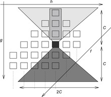
To estimate the maximum number of buckets once more we consider Figure 7.14 as introduced in the analysis of the number of iteration in Symbolic A* (see Ch. 7), in which the g-values are plotted with respect to the h-values, such that nodes with the same  value are located on the same diagonal. For nodes that are expanded in
  the successors fall into
  ,
,  , or
, or  . The number of naughts for each diagonal is an upper bound on the number of buckets that are needed. In Chapter 7, we have already seen that the number is bounded by
  .
.
By the restriction for f-values in the (n2 − 1)-Puzzle only about half the number of buckets have to be allocated. Note that  is not known in advance, so that we have to construct and maintain the files on-the-fly.
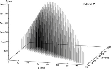
Figure 8.5 shows the memory profile of external A* on a Thirty-Five-Puzzle instance (with 14 tiles permuted). The exploration started in bucket  and terminated while expanding bucket
  . Similar to external BFS but in difference to ordinary A*, external A* terminates while generating the goal, since all states in the search frontier with a smaller g-value have already been expanded. For this experiment three disjoint 3-tile and three disjoint 5-tile pattern databases were loaded, which, together with the buckets for reading and flushing, consumed about 4.9 gigabytes of RAM. The total disk space taken was 1,298,389,180,652 bytes, or 1.2 terabytes, with a state vector of
  bytes: 32 bytes for the state vector plus information for incremental heuristic evaluation; 1 byte for each value stored, multiplied by six sets of at most 12 pattern databases plus 1 value each for their sum. Factor 2 is due to symmetry lookups. The exploration took about two weeks.
The following result restricts duplicate detection to buckets of the same h-value.
Lemma 8.1
In external A* for all  with
with  we have
  .
.
Proof
As in the algorithm of Munagala and Ranade, we can exploit the observation that in an undirected problem graph, duplicates of a node with BFS level i can at most occur in levels i,  , and
, and  . In addition, since h is a total function, we have
  if
if  .
.
For ease of describing the algorithm, we consider each bucket for the Open list as a different file. Very sparse graphs can lead to bad I/O performance, because they may lead to buckets that contain by far less than B elements and dominate the I/O complexity. For the following, we generally assume large graphs for which  and
and  .
.
Algorithm 8.7 depicts the pseudo code of the external A* algorithm for consistent estimates and unit cost and undirected graphs. The algorithm maintains the two values  and
and  to address the currently considered buckets. The buckets of
  are traversed for increasing
  up to
up to  . According to their different h-values, successors are arranged into three different frontier lists:
  ,
,  , and
, and  ; hence, at each instance only four buckets have to be accessed by I/O operations. For each of them, we keep a separate buffer of size
  ; this will reduce the internal memory requirements to M. If a buffer becomes full then it is flushed to disk. As in BFS it is practical to presort buffers in one bucket immediately by an efficient internal algorithm to ease merging, but we could equivalently sort the unsorted buffers for one bucket externally.
There can be two cases that can give rise to duplicates within an active bucket (see Fig. 8.6, black bucket): two different nodes of the same predecessor bucket generating a common successor, and two nodes belonging to different predecessor buckets generating a duplicate. These two cases can be dealt with by merging all the presorted buffers corresponding to the same bucket, resulting in one sorted file. This file can then be scanned to remove the duplicate nodes from it. In fact, both the merging and duplicates removal can be done simultaneously.
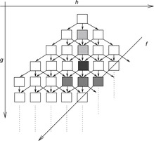
Another special case of the duplicate nodes exists when the nodes that have already been evaluated in the upper layers are generated again (see Fig. 8.6). These duplicate nodes have to be removed by a file subtraction process for the next active bucket  by removing any node that has appeared in
  and
and  (buckets shaded in light gray). This file subtraction can be done by a mere parallel scan of the presorted files and by using a temporary file in which the intermediate result is stored. It suffices to remove duplicates only in the bucket that is expanded next,
  . The other buckets might not have been fully generated, and hence we can save the redundant scanning of the files for every iteration of the innermost while loop.
When merging the presorted sets  with the previously existing Open buckets (both residing on disk), duplicates are eliminated, leaving the sets Open
  , Open
  , and Open
  duplicate free. Then the next active bucket Open
  is refined not to contain any node in Open
  or Open
  . This can be achieved through a parallel scan of the presorted files and by using a temporary file in which the intermediate result is stored, before Open
 is updated. It suffices to perform file subtraction lazily only for the bucket that is expanded next.
Theorem 8.6
(Optimality of External A*) In a unit cost graph external A* is complete and optimal.
Proof
Since external A* simulates A* and only changes the order of expanded nodes that have the same f-value, completeness and optimality are inherited from the properties shown for A*.
Theorem 8.7
(I/O Performance of External A* in Undirected Graphs) The complexity for external A* in an implicit unweighted and undirected graph with a consistent estimate is bounded by  I/Os.
I/Os.
Proof
By simulating internal A*, delayed duplicate elimination ensures that each edge in the problem graph is looked at at most once. Similar to the analysis for external implicit BFS  , I/Os are needed to eliminate duplicates in the successor lists. Since each node is expanded at most once, this adds
  I/Os to the overall runtime. Filtering, evaluating nodes, and merging lists is available in scanning time of all buckets in consideration. During the exploration, each bucket Open will be referred to at most six times, once for expansion, at most three times as a successor bucket, and at most two times for duplicate elimination as a predecessor of the same h-value as the currently active bucket. Therefore, evaluating, merging, and file subtraction add
  I/Os to the overall runtime. Hence, the total execution time is
  I/Os.
I/Os.
If we additionally have  , the complexity reduces to
  I/Os. We next generalize the result to directed graphs with bounded locality.
Theorem 8.8
(I/O Performance of External A* in Graphs with Bounded Locality) The complexity for external A* in an implicit unweighted problem graph with bounded locality and consistent estimate is bounded by  I/Os.
I/Os.
Proof
Consistency implies that we do not have successors with an f-value that is smaller than the current minimum. If we subtract a bucket  from
from  with
with  and
and  being smaller than the locality l, then we arrive at full duplicate detection. Consequently, during the exploration each problem graph node and edge is considered at most once. The efforts due to removing nodes in each bucket individually accumulate to at most
  I/Os, and subtraction adds
  I/Os to the overall complexity.
Internal costs have been neglected in this analysis. Since each node is considered only once for expansion, the internal costs are  times the time
  for successor generation, plus the efforts for internal duplicate elimination and sorting. By setting the weight of all edges
  to
to  for a consistent heuristic h, A* can be cast as a variant of Dijkstra's algorithm that requires internal costs of
  ,
,  successor of
  on a bucket-based priority queue. Due to consistency we have
  , so that, given
  , internal costs are bounded by
  , where
  refers to the total internal sorting efforts.
To reconstruct a solution path, we store predecessor information with each node on disk (thus doubling the state vector size), and apply backward chaining, starting with the target node. However, this is not strictly necessary: For a node in depth g, we intersect the set of possible predecessors with the buckets of depth  . Any node that is in the intersection is reachable on an optimal solution path, so that we can iterate the construction process. The time complexity is bounded by the scanning time of all buckets in consideration, namely by
  I/Os.
I/Os.
Up to this point, we have made the assumption of unit cost graphs; in the rest of this section, we generalize the algorithm to small integer weights in  . Due to consistency of the heuristic, it holds for every node u and every successor v of u that
  . Moreover, since the graph is undirected, we equally have
  , or
, or  ; hence,
  . This means that the successors of the nodes in the active bucket are no longer spread across three, but over
  buckets. In Figure 8.7, the region of successors is shaded in dark gray, and the region of predecessors is shaded in light gray.
For duplicate reduction, it is sufficient to subtract the  buckets
  from the active bucket
  prior to the expansion of its nodes (indicated by the shaded rectangle in Fig. 8.7). We assume
  I/Os for accessing the files is negligible.
Theorem 8.9
(I/O Performance of External A* in Nonunit Cost Graphs) The I/O complexity for external A* in an implicit undirected unit cost graph, where the weights are in  , with a consistent estimate, is bounded by
  .
.
Proof
It can be shown by induction over  that no duplicates exist in smaller buckets. The claim is trivially true for
  . In the induction step, assume to the contrary that for some node
  ,
,  contains a duplicate
  with
with  ; let
; let  be the predecessor of v. Then, by the undirected graph structure, there must be a duplicate
  . But since
  , this is a contradiction to the induction hypothesis.
The derivation of the I/O complexity is similar to the unit cost case; the difference is that each bucket is referred to at most  times for bucket subtraction and expansion. Therefore, each edge in the problem graph is considered at most once.
If we do not impose a bound C on the maximum integer weight, or if we allow directed graphs, the runtime increases to  I/Os. For larger edge weights and
  -values, buckets become sparse and should be handled more carefully.
Let us consider how to externally solve Fifteen-Puzzle problem instances that cannot be solved internally with A* and the Manhattan distance estimate. Internal sorting is implemented by applying Quicksort. The external merge is performed by maintaining the file pointers for every flushed buffer and merging them into a single sorted file. Since we have a simultaneous file pointers capacity bound imposed by the operating system, a two-phase merging applies. Duplicate removal and bucket subtraction are performed on single passes through the bucket file. As said, the successor's f-value differs from the parent node by exactly 2.
In Table 8.3 we show the diagonal pattern of nodes that is developed during the exploration for a simple problem instance. Table 8.4 illustrates the impact of duplicate removal ( ) and bucket subtraction (
 ) for problem instances of increasing complexity. In some cases, the experiment is terminated because of the limited hard disk capacity.
One interesting feature of our approach from a practical point of view is the ability to pause and resume the program execution in large problem instances. This is desirable, for example, in the case when the limits of secondary storage are reached, because we can resume the execution with more disk space.
8.6.5. * Lower Bound for Delayed Duplicate Detection
Is the complexity for external A* I/O-optimal?
Recall the definition of big-oh notation in Chapter 1: We say  if there are two constants
  and c, such that for all
  we have
  . To devise lower bounds for external computation, the following variant of the big-oh notation is appropriate: We say
  if there is a constant c, such that for all M and B there is a value
  , such that for all
  we have
  . The classes
  and
and  are defined analogously. The intuition for universally quantifying M and B is that the adversary first chooses the machine, and then we, as the good guys, evaluate the bound.
External sorting in this model has the aforementioned complexity of  I/Os. As internal set inequality, set inclusion, and set disjointness require at least
  comparisons, the lower bounds on the number of I/Os for these problems are also
  .
.
For the internal duplicate elimination problem the known lower bound on the number of comparisons needed is  , where
  is the multiplicity of record i. The main argument is that after the duplicate removal, the total order of the remaining records is known. This result can be lifted to external search and leads to an I/O complexity of at most
 for external delayed duplicate detection. For the sliding-tile puzzle with two preceding buckets and a branching factor
  we have
  . For general consistent estimates in unit cost graphs we have
  , with c being an upper bound on the maximal branching factor.
Theorem 8.10
(I/O Performance Optimality for External A*) If  , delayed duplicate bucket elimination in an implicit unweighted and undirected graph A* search with consistent estimates that need at least
  I/O operations.
Proof
Since each node gives rise to at most c successors and there are at most three preceding buckets in A* search with consistent estimates in a unit cost graph, given that previous buckets are mutually duplicate free, we have at most  nodes that are the same. Therefore, all sets
  are bounded by
  . Since k is bounded by N we have that
  is bounded by
  . Therefore, the lower bound for duplicate elimination for N nodes is
  .
.
A related lower bound also applicable to the multiple disk model establishes that solving the duplicate elimination problem with N elements having P different values needs at least  I/Os, since the depth of any decision tree for the duplicate elimination problem is at least
  . For a search with consistent estimates and a bounded branching factor, we assume to have
  , so that the I/O complexity reduces to
  .
.
8.7. * Refinements
As an additional feature, external sorting can be avoided to some extent, by a single or a selection of hash functions that splits larger files into smaller pieces until they fit into main memory. As with the h-value in the preceding case a node and its duplicate will have the same hash address.
8.7.1. Hash-Based Duplicate Detection
Hash-based duplicate detection is designed to avoid the complexity of sorting. It is based on either one or two orthogonal hash functions. The primary hash function distributes the nodes to different files. Once a file of successors has been generated, duplicates are eliminated. The assumption is that all nodes with the same primary hash address fit into the main memory. The secondary hash function (if available) maps all duplicates to the same hash address. This approach can be illustrated by sorting a card deck of 52 cards. If we have only 13 internal memory places the best strategy is to hash cards to different files based on their suit in one scan. Next, we individually read each of the files to the main memory to sort the cards or search for duplicates.
The idea goes back to Bucket Sort. In its first phase, real numbers  are thrown into n different buckets
  . All the lists that are contained in one bucket can be sorted independently by some other internal sorting algorithm. The sorted lists for
  are concatenated to a fully sorted list. In the worst case, each element is thrown into the same bucket, such that Bucket Sort does not improve the sorting. However, in the average case, the (internal) algorithm is much better. Let
  be a random variable that denotes how many elements fall into bucket i; that is,
  denotes the length of bucket list
  . For every bucket we might assume that the probability that an element falls into bucket
  for
for  is
is  . Therefore,
  follows a binomial distribution with parameters n and
  . The mean is
  and the variance is
  .
.
By iterating Bucket Sort, it is not difficult to come up with an external version of Radix Sort that scans the files more than once according to a radix representation of the key values. We briefly illustrate how it works. Say that we have some numbers in the range of 0 and 99, say 48, 26, 28, 87, 14, 86, 50, 23, 34, 69; and 17 in decimal (10-ary) representation. We devise 10 buckets  , representing the numbers
  . We have two distribution and collection phases. In the first phase we distribute according to the right-most decimal, yielding
  ,
,  ,
,  ,
,  ,
,  ,
,  ,
,  ,
,  ,
,  , and
, and  . We collect the data by scanning 50, 23, 14, 34, 26, 86, 87, 17, 48, 28, 69, and distribute this set according to the left-most decimal, yielding
  ,
,  ,
,  ,
,  ,
,  ,
,  ,
,  ,
,  ,
,  , and
, and  for a final scan that produces the sorted outcome.
For the Fifteen-Puzzle problem in ordinary vector representation with a number for each board position, we have 16 phases for radix sort using 16 buckets.
If we have N data elements with a radix representation of length l with base b then the internal time complexity of Radix Sort is  , and the internal space complexity
  . Since all operations can be buffered, the external time complexity reduces to
  I/Os. Since we may assume that the number b of buckets needed is small, we have an improvement to External Mergesort, if
  .
.
8.7.2. Structured Duplicate Detection
Structured duplicate detection incorporates a hash function that maps nodes into an abstract problem graph; this reduces the successor scope of nodes that have to be kept in main memory. Such hash projections are state space homomorphisms (as introduced in Ch. 4), such that for each pair of consecutive abstract nodes the pair of original nodes are also connected. A bucket now corresponds to the set of original states, which all map to the same abstract state. In difference to delayed duplicate detection, structured duplicate detection detects duplicates early, as soon as they are generated. Before expanding a bucket, not only the bucket itself, but all buckets that are potentially affected by successor generation have to be loaded and, consequently, fit into main memory.
This gives rise to a different definition of locality, which determines a handle for the duplicate detection scope. In difference to the locality for delayed duplicate detection the locality for structured duplicate detection is defined as the maximum node branching factor  in the abstract state space
  .
.
If there are different abstractions to choose from, a suggestion is to take those that have the smallest ratio of maximum node branching factor  and abstract state space size
  . The idea is that smaller abstract state space sizes should be preferred but usually lead to larger branching factors.
In the example of the Fifteen-Puzzle (see Fig. 8.8), the projection is based on nodes that have the same blank position. This state space abstraction also preserves the additional property that the successor set and the expansion sets are disjoint, yielding no self-loops in the abstract problem graph. The duplicate scope defines the successor buckets that have to be read into main memory.
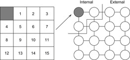
The method is crucially dependent on the availability and selection of suitable abstraction functions  that adapt to the internal memory constraints. In contrast, delayed duplicate detection does not rely on any partitioning beside the heuristic function and it does not require the duplicate scope to fit in the main memory.
Structured duplicate detection is compatible with ordinary and hash-based duplicate detection; in case the files that have to be loaded into the main memory no longer fit, we have to delay. However, the structured partitioning may have truncated the file sizes for duplicate detection to a manageable number. Each heuristic or hash function defines a partitioning of the search space but not all partitions provide a good locality with respect to the successor or predecessor states. State space abstractions are specialized hash functions in which we can study the successor relationship.
8.7.3. Pipelining
Many external memory algorithms arrange the data flow in a directed acyclic graph, with nodes representing physical sources. Every node writes or reads streams of elements.
Pipelining is a technique inherited from the database community, and improves algorithms that read data from and write data to buffered files. Pipelining allows algorithms to feed the output as a data stream directly to the algorithm that consumes the output, rather than writing it to the disk first.
Streaming nodes is equivalent to scan operations in nonpipelined external memory algorithms. The difference is that nonpipelined conventional scanning needs a linear number of I/Os, whereas streaming often does not incur any I/O, unless a node needs to access external memory data structures.
The nonpipelined and pipelined version of external breadth-first search are compared in Figure 8.9. In the pipelined version the whole algorithm is implemented in one scanner module that reads the nodes in  and
and  and scans through the stream in just one pass, and outputs the nodes in the current level
  and the multiset
  , which is passed directly to the sorter. The output of the sorter is scanned once to delete duplicates and its output is used as
  in the next iteration.
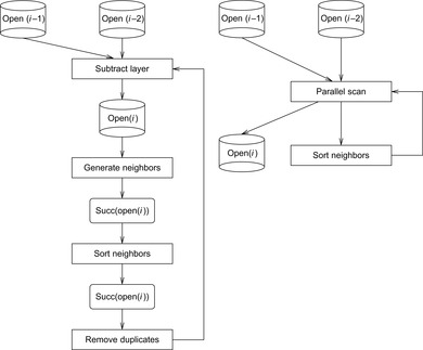
8.7.4. External Iterative-Deepening A* Search
While external A* requires a constant amount of memory for the internal read and write buffers, IDA* requires very little memory that scales linear with the search depth. External A* removes all duplicates from the search, but to succeed it requires access to disk, which tends to be slow. Moreover, in search practice disk space is limited, too. Therefore, one option is to combine the advantages of IDA* and external A*.
As a first observation, pruning strategies for IDA* search (e.g., omitting predecessors from the successor lists) can help save external space and access time. The reason is that when detecting duplicates late, larger amounts of disk space may be required for generating them.
The integration of IDA* in external A* is simple. Starting with external A*, the buckets up to a predefined f-value  (the split value) are generated. Then with increasing depth all buckets on the
  diagonal are read, and all states contained in the buckets are fed into IDA* as initial states, which is initialized to an anticipated solution length
  . As a side effect of all such runs being pairwise independent they can be easily distributed (e.g., on different processor cores).
Table 8.5 shows the results of solving a Twenty-Four-Puzzle instance according to different f-value splits to document the potential of such hybrid algorithms. In another instance (with an optimal step plan of 100 moves) a split value of 94 generated 367,243,074,706 nodes using 4.9 gigabytes on disk. A split value of 98 resulted in 451,034,974,741 generated nodes and 169 gigabytes on disk. We see that there is potential savings based on the different ordering of moves. By its breadth-first ordering, external A* necessarily expands the entire  -diagonal, whereas by its depth-first ordering IDA* does not need to look at all states in the
  -diagonal. It can stop at the first goal found.
8.7.5. External Explicit-State Pattern Databases
External pattern databases correspond to complete explorations of abstract state spaces. Most frequently they correspond to external BFS with delayed duplicate detection. The construction of external pattern databases is especially suited to frontier search, as no solution path has to be reconstructed.
During construction each BFS layer i has been assigned to an individual file  . All states in
  have the same goal distance, and all states that map to a state in i share the heuristic estimate i. For determining the h-value for some given state u in algorithms like external A* we first have to scan the files to find u.
As this is a cost-intensive operation, whenever possible, pattern database lookup should be delayed, so that the heuristic estimates for a larger set of states can be retrieved in one scan. For example, external A* distributes the set of successor states of each bucket according to their heuristic estimates. Hence, it can be adapted to delayed lookup, intersecting the set of successor states with (the state set represented by) the abstract states in the file of a given h-value.
To keep the pattern database partitioned, we have to assume that the number of files that can be opened simultaneously does not exceed  . We observe that
  matches the locality of an abstract state space graph.
Theorem 8.11
(Complexity External Pattern Databases Search) In an unweighted problem graph  with pattern database abstraction
  external A* with bounded concrete and abstract locality requires
  I/Os.
I/Os.
Proof
Constructing the pattern database externally yields  I/Os, whereas external A* without external pattern database lookups requires
  I/Os. If we sort the successors with respect to the sorting criteria that has been used to generate the abstract state space we can evaluate the entire successor set in one scan of the entire external pattern database. As we look at most
  buckets in external A*, this gives a trivial bound of
  I/Os. In case of graphs with bounded locality at most a constant number of pattern database files are addressed for each successor set, such that each file is considered as a candidate for a lookup at most
  times. Moreover, each successor set is additionally scanned at most a constant number of times. Hence, the additional work for pattern database lookup is
  I/Os. In total, we arrive at
  I/Os.
I/Os.
Note that external breadth-first heuristic search with optimal bound  directly leads to
  I/Os, but iteratively searching for
  is involved.
Can we avoid the additional sorting requests on the successor set? One solution is to already sort the successor sets in original space according to the order in abstract space. To allow full duplicate elimination, synonyms have to be disambiguated. A hash function h will be called order preserving, if for all u in original space  implies
  . For a pattern database heuristics it not difficult to obtain an order-preserving hash function. In concrete space with state comparison function
  we can include any hash function
  that has been used to order the states in abstract space as a prefix to
  . We extend state u to
  and define
  if either
  or
or  and
and  .
.
When using maximization over multiple-pattern databases, a hash function that is order preserving with respect to more than one abstraction is more difficult to obtain. However, successive projection and resorting always works. As the successor sets for resorting have no duplicates, external sorting can be attributed to the set V not to E. For this case, the number of pattern databases k leads to the overall complexity of  I/Os.
I/Os.
If a heuristic estimate is needed as soon as a node is generated, an appropriate choice for creating external memory pattern databases is a backward BFS with structured duplicate detection, as structured duplication already provides locality with respect to a state space abstraction function. Afterwards, the construction patterns are arranged according to pattern blocks, one for each abstract state. When a concrete heuristic search algorithm expands nodes, it must check whether the patterns from the pattern-lookup scope are in the main memory, and if not, it reads them from disk. Pattern blocks that do not belong to the current pattern-lookup scope are removed. When the part of internal memory is full, the search algorithm must decide which pattern block to remove from internal memory, for example, by adopting the least-recently used strategy.
8.7.6. External Symbolic Pattern Databases
Symbolic pattern databases can also be constructed externally. Each BFS level (in the form of a BDD) can be flushed to disk, so that the memory for representing this level can be reused. Again the heuristic is partitioned into files and pattern database lookup in algorithms like external A* is delayed.
As the BDD representation of a state set is unique, during symbolic pattern database construction no effort for eliminating duplicates in one BFS level is required. Before expanding a state set, however, we have to apply duplicate detection with regard to previous BFS levels. If this is too expensive in some critical level, we may afford some states to be represented more than once, but have to ensure termination.
For the construction of larger pattern databases, the intermediate result of the symbolic successor sets (the image) can also become too large to be completed in the main memory. As a solution, we can compute all subimages individually (one for each individual action), flush them, and externally compute their disjunction (e.g., in the form of a binary tree) in a separate program.
8.7.7. External Relay Search
Even if all refinements are played, the external exploration might still be too heavy to complete on disk. Besides starting from scratch with some approximate search, relay search can be directly applied to the best search bucket(s) found on an completed f-diagonal. All other buckets are eliminated from the search. As a result a lower and upper bound on the problem instances are produced.
Figure 8.10 illustrates the memory profile for a relay solution that solves fully random instances of the Thirty-Five-Puzzle with symbolic pattern databases. We observe three exploration peaks, where the search consumed too much resources and it was restarted with the currently best solution buckets. Starting with an initial estimate 152 as a lower bound the obtained range for the optimal solution was  . The large-scale exploration consumed
  bytes (
 terabytes).
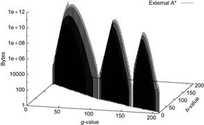
8.8. * External Value Iteration
We now discuss an approach for extending the search model to cover uncertainty. More precisely, we extend the value iteration procedure (introduced in Ch. 2) to work on large state spaces that cannot fit into the RAM. The algorithm is called external value iteration. Instead of working on states, we work on edges for reasons that shall become clear soon. In our case, an edge is a 4-tuple where u is called the predecessor state, v the stored state, a the action that transforms u into v, and
  is the current assignment of the value function to v. Clearly, v must belong to
  . In deterministic problems, v is determined by u and a and so it can be completely dropped, but for the nondeterministic problems, it is a necessity.
Similarly to the internal version of value iteration, the external version works in two phases. A forward phase, where the state space is generated, and a backward phase, where the heuristic values are repeatedly updated until an  -optimal policy is computed, or
  iterations are performed.
We will explain the algorithm in a running example using the graph in Figure 8.11. The states are numbered from 1 to 10, the initial state is 1, and the terminal states are 8 and 10. The numbers next to the states are the initial heuristic values.

8.8.1. Forward Phase: State Space Generation
Typically, a state space is generated by a depth-first or a breadth-first exploration that uses a hash table to avoid reexpansion of states. We choose an external breadth-first exploration to handle large state spaces. Since in an external setting a hash table is not affordable, we rely on delayed duplication detection. It consists of two phases, first removing duplicates within the newly generated layer, and then removing duplicates with respect to previously generated layers. Note that an edge  is a duplicate if and only if its predecessor u, its state v, and the action a match an existing edge. Thus, in undirected graphs, there are two different edges for each undirected edge. In our case, sorting-based delayed duplicate detection is best suited as the sorted order and is further exploited during the backward phase.
Algorithm 8.8 shows external value iteration in pseudo code. For each depth value d the algorithm maintains the BFS layers  on disk. The first phase ends up by concatenating all layers into one
  list that contains all edges reachable from s. For bounded locality, the complexity of this phase is
  I/Os.
I/Os.
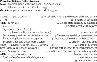
8.8.2. Backward Phase: Update of Values
This is the most critical part of the approach and deserves more attention. To perform the update on the value of state v, we have to bring together the value of its successor states. Because they both are contained in one file, and there is no arrangement that can bring all successor states close to their predecessor states, we make a copy of the entire graph (file) and deal with the current state and its successor differently. To establish the adjacencies, the second copy, called  , is sorted with respect to the node u. Remember that
  is sorted with respect to the node v.
A parallel scan of files  and
and  gives us access to all the successors and values needed to perform the update on the value of v. This scenario is shown in Figure 8.12 for the graph in the example. The contents of Temp and
  , for
, for  , are shown along with the heuristic values computed so far for each edge
  . The arrows show the flow of information (alternation between dotted and dashed arrows is just for clarity). The results of the updates are written to the file
  containing the new values for each state after
  iterations. Once
  is computed, the file
  can be removed since it is no longer needed.
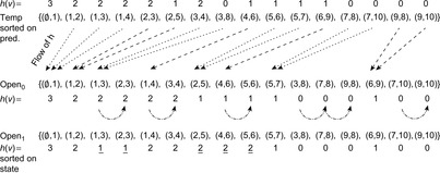 |
| Figure 8.12 |
Algorithm 8.9 shows the backward update algorithm for the case of MDP models; the other models are similar. It first copies the  list in
  using buffered I/O operations, and sorts the new
  list according to the predecessor states u. The algorithm then iterates on all edges from
  and searches for the successors in
  . Since
  is sorted with respect to states v, the algorithm never goes back and forth in any of the
  or
or  files. Note that all reads and writes are buffered and thus can be carried out very efficiently by always doing I/O operations in blocks.
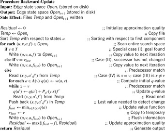
We now discuss the different cases that might arise when an edge  is read from
  . States from Figure 8.11 that comply with each case are referred to in parentheses. The flow of the values in h for the example is shown in Figure 8.12.
• Case I: v is terminal (states 8 and 10). Since no update is necessary, the edge can be written to  .
.
• Case II: v is the same as the last updated state (state 3). Write the edge to  with this last value. (Case shown in Figure 8.12 with curved arrows.)
• Case III: v has no successors. That means that v is a terminal state and so is handled by case I.
• Case IV: v has one or more successors (remaining states). For each action  , compute the value
  by summing the products of the probabilities and the stored values. Such value is kept in the array
  .
.
For edges  read from
  , we have:
• Case A: y is the initial state, implying  . Skip this edge since there is nothing to do. By taking
  as the smallest element, the sorting of
  brings all such edges to the front of the file. (Case not shown for sake of brevity.)
The array  is initialized to the edge weight
  , for each
  . Once all the successors are processed, the new value for v is the minimum of the values stored in the q-array for all applicable actions.
An important point to note here is that the last edge read from  isn't used. The operation Push-back puts back this edge into
  . This operation incurs in no physical I/O since the
  file is buffered. Finally, to handle case II, a copy of the last updated node and its value are stored in variables
  and
and  , respectively.
Theorem 8.12
(I/O Complexity External Value Iteration) Assuming bounded locality the algorithm external value iteration performs at most  I/Os.
I/Os.
Proof
For bounded locality, the forward phase requires  I/Os. Moreover, the backward phase performs at most
  iterations. Each such iteration consists of one sorting and two scanning operations for a total of
  I/Os.
I/Os.
As an example domain we consider the sliding-tile puzzle, performing two experiments: one with deterministic moves, and the other with noisy actions that achieve their intended effects with probability  and no effect with probability
  . The rectangular
  sliding-tile puzzle cannot be solved with internal value iteration because the state space did not fit in RAM. External value iteration generated a total of 1,357,171,197 edges taking 45 gigabytes of disk space. The backward update has finished successfully in 72 iterations using 1.4 gigabytes RAM. The value function for initial state converged to 28.8889 with a residual smaller than
  .
.
8.9. * Flash Memory
Mechanical hard disks have provided us with reliable service over these years. Their dominance at least on mobile devices is about to change with the advent of solid state disk (SSD). An SSD is electrically, mechanically, and software compatible with a conventional (magnetic) hard disk drive. The difference is that the storage medium is not magnetic (like a hard disk) or optical (like a CD), but a solid state semiconductor (NAND flash) such as a battery-backed RAM or other electrically erasable RAM-like chip. In the last few years, NAND flash memories outpaced RAM in terms of bit density, and the market with SSDs continues to grow. This provides faster access time than a disk because the data can be randomly accessed and does not rely on a read/write interface head synchronizing with a rotating disk. Typical values for data transfer bandwidth and access time for both magnetic and solid state disks is shown in Figure 8.13. (These values are, of course, subject to hardware changes, where SSDs seem to advance faster than HDDs.)
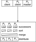
The speed of random reads for an SSD built with NAND flash memory lies roughly at the geometric mean of the speeds of RAM and a magnetic hard disk drive (HDD). The only factor limiting SSDs from being massively spread is the cost of the device if expressed per stored bit. The cost per stored bit is still significantly higher for SSDs than for magnetic disks.
We observe that random read operations on SSDs are substantially faster than on mechanical disks, while other parameters are similar. Therefore, it appears natural to ask whether it is necessary to employ delayed duplicate detection (DDD) known from the current I/O-efficient graph search algorithms, or if is possible to build an efficient SSD algorithm using standard immediate duplicate detection (IDD), hashing in particular.
Note that the external memory model is no longer a good match, since it does not cover the different access times for random read and write operations. For SSDs, therefore, it is suitable to extend the external memory model just introduced. One option is to work with different buffer sizes for read and write. Another option that we have chosen is to include a penalty factor p for random write operations.
There are different options to exploit SSDs in state space search. First, we study direct access to the SSD without exploiting RAM. This implies both random read and random write operations. The implementation serves as a reference, and can be scaled to any implicit graph search with a visited state space that fits on the SSD. As an improvement, a bit-state table in RAM can then be used to avoid unsuccessful lookups.
Next, we compress the state in internal memory to include the address on secondary memory. For this case, states are written sequentially to the external memory in the order of generation. For resolving hash synonyms, state lookups in the form of random reads are needed. Even though linear probing shows performance deficiencies for internal hashing, for blockwise strategies, it is the apparent candidates. Alternative hashing strategies can further reduce the number of random reads.
The third approach flushes the internal hash table to the external device once it becomes full. In this case, full state vectors are stored internally. For large amounts of external memory and small vector sizes, large state spaces can be looked at. Usually the exploration process is suspended while flushing the internal hash table. We observe different trade-offs for the amount of randomness for reading and writing, which mainly depend on increasing the locality of the access.
8.9.1. Hashing
The general setting (see Fig. 8.14) is a background hash table  kept on the SSD, which can hold
  entries. We additionally assume a foreground hash table
  with
with  entries. The ratio between foreground and background is, therefore,
  . Collisions especially on the background hash table can yield additional burden. As chaining requires overhead for storing and following links, we are left with open addressing and adequate probing strategies.
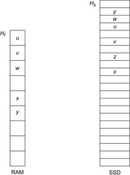
As indicated earlier, SSDs prefer sequential writes and sequential reads, but can cope with an acceptable number of random reads. As linear probing finds elements through sequential scanning, it is I/O efficient. For load factor  , a successful search requires about
  accesses on the average, but an unsuccessful search requires about
  accesses on the average. For a hash table that is filled up to
  % we have less than three states to look at on the average, which easily fit into the I/O buffer. Given that random access is slower than sequential access, this implies that unless the hash table becomes filled, linear probing with one I/O per lookup per node is an appropriate option for SSD-based hashing.
8.9.2. Mapping
The simplest method to apply SSDs in graph search is to store each node at its background hash address in a file, and if occupied, to apply a conflict resolution strategy on disk. By their large seek times, this option is clearly infeasible for HDDs, but it does apply to some extent to SSDs. Nonetheless, besides extensive use of random writes that operate blockwise and are, thus, expected to be slow, one problem of the approach is the initialization time, incurred by erasing all existing data stored in the background hash table.
Hence, we apply a refinement to speed up search. With one additional bitvector array kept in RAM, we denote whether or not a state is already stored on disk. This limits initialization time to reset all bits in main memory, which is much faster. Moreover, this saves lookup time in case of hashing a new state with an unused table entry. Figure 8.15 (left) illustrates the approach. The bitvector occupied memorizes, if the address on the SSD is in use.
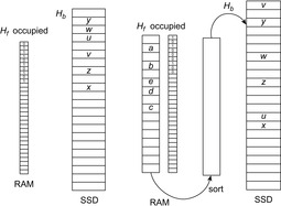
The extra amount of RAM additionally limits the size of the search spaces to be processed. In search practice with a full state vector of several hundred bytes to be stored in the background hash table, however, investing one bit per state in RAM does no harm, given that the ratio between main and external memory remains moderate. The only limit for the exploration is imposed by the number of states that can be stored on the solid state disk, which we assume to be sufficiently large.
For analyzing the approach, let n be the number of nodes and e be the number of edges in the state space graph that are looked at. Without occupied vector, this requires e lookup and n insert operations. Let B be the size of a block (amount of data retrieved, or written with one I/O operation) and  be the fixed length of the state vector. As long as
  , at most two blocks are read for each lookup (when linear probing arrives at the end of the table, an additional seek to the start of the file is needed). For
  no additional random read access is necessary. After the lookup, an insert operation results in one random write. This results in a flash I/O complexity of
  , where p is the penalty factor for random write operations. Using the occupied vector, the number of read operations reduces from e to n, assuming that no collisions take place.
As the main bottleneck of the approach is random writing to the background hash table, as another refinement we can additionally employ a foreground hash table as a write buffer. Due to numerous insert operations, the foreground hash table will become filled, and then has to be flushed to the background, which incurs writes and subsequent reads. One option that we call merging is to sort the internal hash table with regard to the external hash function before flushing. If the hash functions are correlated, the sequence is already presorted, by means that the number of inversions  is small. If
  is small we use an algorithm like adaptive sort that exploits presorting. While flushing we now have a sequential write (due to the linear probing strategy), such that the total worst-case I/O time for flushing is bounded by the number of flushes times the efforts for sequential writes. Figure 8.15 (right) illustrates the approach. Since we are able to exploit sequential data processing, updating the background hash table corresponds to a scan (see Fig. 8.16). Blocks are read into the RAM and merged with the internal information and then flushed back to SSD.

8.9.3. Compressing
Here we store all state vectors in a file on the external storage device, and substitute the state vector by its relative file pointer position. For an external hash table of size m this requires  bits per entry and
  bits in total. Figure 8.17 illustrates the approach with arrows denoting the position on external memory. An additional bitvector is no longer needed.
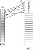
This strategy also results in e lookups and n insert operations. Since the ordering of states on the SSD does not necessarily correlate with the order in main memory, the lookup of states due to linear probing induces multiple random reads. Hence, the amount of individual blocks that have to be read is bounded by  . In contrast, all insert operations are performed sequentially, utilizing a cache of B bytes in memory. Subsequently, this approach performs
  random reads to the SSD. As long as
  this approach performs less random read operations than mapping. By using another internal hashing strategy, for example, cuckoo hashing (see Ch. 3), we can reduce the maximum number of lookups to 2. As sequential writing of n states of s bytes requires
  I/Os, the total flash-memory I/O complexity is
  .
.
8.9.4. Flushing
The previous approaches either require significant time to write data according to  or request significant sizes of foreground memory. There are further trade-offs that we will consider next.
One first solution, called padding, appends the entire foreground hash table as it is to the existing data on the background table. Hence, the background hash function can be roughly characterized as  , where i denotes the current number of flushes, and s the state to be hashed.
Writing is sequential, and conflict resolution strategy is inherited from the internal memory. For several flushing readings, a state for answering membership queries becomes involved, as the search for one state incurs up to r many table lookups. Conflict resolution may lead to an even worse performance. For a moderate number of states that exceed RAM resources only by a very small factor, however, the average performance is expected to be good. As far as all states can reside in main memory no access to the background hash table is needed.
We can safely assume that load factor  is small enough, so that the extra amount of work due to linear probing is transparent by using block accesses. Again, e lookups and n insert operations are performed. Let
  be the number of successors generated in phase i,
  . For phase 0 no access to the background table is needed. For phase i,
  , at most
  blocks have to be read. Together with the sequential write of n elements (in r rounds) this results in a flash-memory complexity of
  I/Os. An illustration is provided in Figure 8.18 (left). The entire foreground hash table has been flushed once, and the maximum number of flushes is set to 3.
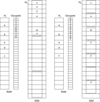
The obvious alternative is to slice the background hash table, such that  becomes
  plus the number of flushes. An illustration is provided in Figure 8.18 (right); this is the situation after one flush, and again, at most three flushes are assumed.
The disadvantage of processing the entire external hash table during flushing is compensated by the fact that the probing sequences in the hash tables can now be searched concurrently. For the lookup we use a bit vector (of size equal to the number of flushes) that monitors if an individual probing sequence has terminated with an empty bucket. If all probing sequences fail, the query itself has failed.
8.10. Summary
By the rapid increase in size and sequential access time and the rapid decrease in prices, in this chapter we have studied external (memory) search algorithms that explore the problem graph by utilizing hard disks.
Graph search algorithms, such as BFS, depth-first search, and A*, use duplicate detection to recognize when the same node is reached via alternative paths in a graph. This traditionally involves storing already explored nodes in random access memory (RAM) and checking newly generated nodes against the stored nodes. However, the limited size of RAM creates a memory bottleneck that severely limits the range of problems that can be solved with this approach. All clever techniques that have been developed for searching with limited RAM eventually are limited in terms of scalability, and many practical graph search problems are too large to be solved using any of these techniques. Relying on virtual memory slows down the exploration due to an excessive number of page faults. We have shown that the scalability of graph search algorithms can be dramatically improved by using external memory, such as a disk, to store generated nodes for use in duplicate detection. However, this requires very different search strategies to overcome the six orders-of-magnitude difference in random access speed between RAM and disk.
Disk access is supervised by the exploration algorithms rather than by the underlying operating system. Thus, the algorithm design is mainly concerned about access locality. Efficient designs provide alternative implementations to an internal hash table and allow a delayed detection of duplicates. If disk space becomes sparse, early merging delayed duplicate detections is invoked on demand. In hash-based duplicate detection coarse hash codes are effective for accelerating external sorting. If according to the hash value, the neighboring sets fit into main memory, so-called structured duplicate detection ensures that all duplicates are caught in the RAM.
The partitioning of the state space into buckets has much in common with the symbolic (blind and heuristic) search algorithm in Chapter 7. As the exploration is explicit-state, duplicates within one bucket have to be found by external sorting followed by an external scan operation.
External BFS was discovered for explicit graph search, but is much more effective in implicit graph search because no access to the adjacency list is required. Some algorithmic techniques such as preprocessing the explicit graph become obsolete, while others like pipelining become more attractive. Using one file as a queue, external BFS is I/O optimal in undirected graphs (either sparse or not). When looking at directed graphs, once again, the locality of the problem graphs becomes the important measurement to determine the duplicate detection scope. Besides the sorting it influences the I/O complexity the most.
Given the optimal solution bound, external A* and external breadth-first heuristic search both operate with a growing g-value and thus explore the same state sets. Although external A* has some difficulties in obtaining optimal efficiency in very sparse graphs (e.g., a chain of states) inducing extremely long solutions (file buffers are needed for every active bucket), external breadth-first heuristic search will have difficulties when searching with an unknown solution depth (for a rising threshold new states hardly squeeze in existing files).
We have extended external memory search from deterministic to the general search model that includes nondeterministic and probabilistic search spaces, like MDPs. Different to the deterministic setting, the external value iteration algorithm generates the entire set of reachable states, requires many passes over the problem graph, and operates on the problem graph edges instead of the problem graph nodes.
Table 8.6 gives an overview of the external algorithms presented in this chapter. To ease the denotation of the complexities, we assume constant locality as implied be undirected graph structures and use  to abbreviate
  . Nonetheless, most algorithms extend to integer edge weights and directed graphs. In directed graphs, a larger set of buckets has to be traversed to subtract duplicates from earlier search levels. In weighted graphs, nonadjacent buckets have to be addressed. Explicit graph search is only efficient for regular graph subclasses. For external BFS and external A* with delayed duplicate detection we have a matching lower bound.
| Name | I/O Complexity | Weight | Graph | Optimal |
|---|---|---|---|---|
| MR (8.1) | uniform | undirected | √ | |
| MM | uniform | undirected | √ | |
| Ext.-SSSP | regular | √ | ||
| Ext.-BFS (8.2) | uniform | undirected | √ | |
| Ext.-A* (8.7) | uniform | undirected | √ | |
| Ext.-PDB-A* | ||||
| uniform | undirected | √ | ||
| Ext.-BFBnB (8.4) | undirected | √ | ||
| Ext.-BFHS (8.4) | uniform | undirected | √ | |
| Ext.-EHC (8.5, 8.6) | undirected | - | ||
| Ext.-SDD | uniform | structured | √ | |
| Ext.-VI (8.8, 8.9) | general | structured | √ |
Structured duplicate detection is assigned to an I/O complexity of  , which is apparent if the projection function is the identity. In theory, such worst-case performance can occur in any abstraction that forces singleton nodes to be retrieved from disk. In terms of cache-oblivious algorithms, it is worth mentioning that the localized exploration that uses RAM and hard disks also optimizes the CPU cache performance.
With the advent of solid state disk technology, immediate duplicate detection becomes tractable, offering more flexibility for the choice of the exploration strategy. Monitoring CPU performances suggests that I/O waits are present, but not thrashing. With SSDs' random access time decreasing, SSDs will likely become fast enough to rise the CPU usage to full speed making the SSD fully transparent to the user. Compression, likely the best performing strategy, requires substantial main memory, which according to current ratios of space between RAM and SSDs is still no bottleneck.
8.11. Exercises
8.1 For an external stack, the buffer is an internal memory array of  elements that at any time contains the
  elements most recently inserted. We assume that the stack content is bounded by at most N elements.
1. Implement a remove operation with no I/O, except for the case when the buffer has run empty. In this case a single I/O to retrieve a block of B elements is allowed.
2. Implement an insert operation with no I/O, except for the case when the buffer has run full. In this case a single I/O to write a block of B elements is allowed.
3. Show that insertion and deletion take  I/Os in the amortized sense.
4. Why does a stack not use a buffer of size B, but  instead?
5. Implement an external queue using two stacks to achieve  I/Os amortized for insertion and deletion.
8.2 An external linked list preserves locality: Elements that are near each other in the list must tend to be stored in the same block.
1. Show that a simple approach of putting B consecutive elements in each block yields a list scan of N elements in  I/Os.
I/Os.
2. Show that such a simple implementation requires  I/Os for insertion and deletion.
8.3 A refined implementation of an external linked list maintains the following invariant: There are more than  elements in every pair of consecutive blocks.
1. Show that the number of I/Os for a sequential scan grows by at most a factor of three.
2. If either neighbor of the block for an insertion is full, we split the block into two blocks of at most  elements. Show that the invariant is maintained.
3. If one of the neighbors of the block for a deletion has  elements or less, we merge the two blocks. Show that the invariant is maintained.
5. Show that this approach ensures a constant number of I/Os to update a linked list.
6. Show that this approach gives  I/Os for N consecutive inserts.
7. Show that after an insertion at least  deletions are needed to violate the invariance.
8. Increase the space utilization from 1/3 to 1/ϵ.
8.4 Suppose we are given three large arrays A, B, and C of size n that exceed main memory. Moreover C is a permutation  . The task is to assign
  to
to  for
for  .
.
1. Show that the naive approach of sequentially processing the input implies  I/Os.
I/Os.
2. Devise a strategy that has an I/O complexity of  .
.
8.5 Let the BFS number be the order of node visits in a BFS traversal and the BFS tree be the tree associated with a BFS search. (For each node v the parent of v in the BFS tree is the node with  .) Show that for undirected graphs the following transformation can be done using
  I/Os:
I/Os:
1. BFS numbers in BFS tree.
2. BFS tree in BFS level.
3. BFS level in BFS numbers.
8.6 As a simple external implementation of a balanced binary search tree incurs  I/Os, B-trees have been proposed as a generalization to trees of degree
  . For external usage, a B -tree node guides searches to one of the
  subtrees. The balance invariant requires that (1) for every node at level i smaller than the height of the tree h the number of leaves below are at least
  and (2) for every node at level
  the number of leaves below is at most
  . Show that the balance invariant implies the following assertions:
1. Any node has at most  children.
2. The height of the B -tree is at most  .
.
3. Any nonroot node has as at least  children.
4. Infer that the worst case for searching a B -tree is  I/Os.
I/Os.
5. Show a lower bound of  on the height of the B -tree.
6. Explain how to perform insertions and deletions in  I/Os.
I/Os.
8.7 Explain the working of the algorithm of Munagala and Ranade with respect to the graph in Figure 8.19 starting at node 1. What are the generated nodes in  for
for  ? For each iteration remove the duplicates in this set and display the nodes that are remaining. For each iteration remove the lists
  and
and  .
.
8.8 Derive an external implementation of the implicit version of the Bellman-Ford algorithm (see Ch. 2) that uses  I/Os, where k is the length of the cost-optimal solution path. You may restrict to undirected unit cost problem graphs. Use a derivate of Munagala and Ranade's external BFS implementation and restrict duplicate elimination to allow reopening. Show that each edge and each node is considered at most k times to arrive at the stated complexity.
8.9 Show that the number of buckets  that are considered by external A* in a unit cost problem graph with a consistent heuristic is bounded by
  .
.
8.10 Give a pseudo-code implementation for external BFS exploration for cost-optimizing search, incrementally improving an upper bound U on the solution cost. The state sets that are used should be represented in the form of files. The search frontier denoting the current BFS layer is tested for an intersection with the goal, and this intersection is further reduced according to the already established bound.
8.11 Show that external A* with one pattern database heuristic can be executed in  I/Os. (The only change is the factor
  compared to
  in the text.)
8.12 The Pancake problem is defined as follows. Given an n-stack of pancakes of different sizes, how many flips of the first k pancakes are needed to get them into ascending order? The problem is illustrated in Figure 8.20. It is known that  flips alway suffice, and that
  is a lower bound. In the Burned Pancake the pancakes are burned on one side and the additional requirement is to bring all burned sides down. It is known that
  flips always suffice and that
  is a lower bound.
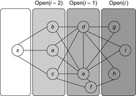

1. Show that by iteratively putting the next largest element in its proper place we can obtain a solution with  flips, and when the initial permutation has none of the desired adjacencies, at least n flips are needed.
2. An unproven conjecture for the Burned Pancake problem is that the worst-case scenario is the original stack with all burned sides up. Validate it for  .
.
3. Derive a heuristic for the Pancake problem that is defined on the number of times the order changes from smaller to larger pancakes and vice versa.
4. Solve the problem with external BFS up to  for the ordinary and up to
  for the Burned Pancake problem. How far can you scale with external A* search?
8.12. Bibliographic Notes
The single disk model for external memory algorithms has been invented by Aggarwal and Vitter (1988). A detailed introduction has been given by Sanders, Meyer, and Sibeyn (2002). The buffer tree data structure is due to Arge (1996). A number of other variants for external priority queues have been suggested in the literature (Kumar and Schwabe, 1996; Fadel et al., 1997; Brengel et al., 1999). The tournament tree and its application to graph search has been proposed by Kumar and Schwabe (1996) and the buffered repository tree and its use in external graph search has been studied in Buchsbaum, Goldwasser, Venkatasubramanian, and Westbrook (2000).
There is no major difference in the application algorithm of Munagala and Ranade (1999) for explicit and implicit graphs. However, the precomputation and access efforts are by far larger for the explicit graphs. The extension to the algorithm proposed by Mehlhorn and Meyer (2002) has been the first attempt to break the O(|V|) I/O barrier for explicit graphs. The I/O lower bound for delayed duplicate detection refers to Aggarwal and Vitter (1987), who have given such a lower bound for external sorting. Arge, Knudsen, and Larsen (1993) has extended this work to the issue of duplicate detection.
The term delayed duplicate detection has been coined by Korf (2003a) in the context of complete BFS explorations of rectangular  -Puzzles. As said in the text, the approach shares similarities with internal frontier search. As said in the text, the approach shares similarities with internal frontier search by Korf, Zhang, Thayer, and Hohwald (2005). In the published exposition of Korf (2003a), the elimination of nodes with respect to previous lists is mentioned. External sorting based on hash functions (hash-based delayed duplicate detection) has been proposed in the context of complete BFS of the Fifteen-Puzzle by Korf and Schultze (2005). For permutation games like Pancake and Burned Pancake, already considered by Gates and Papadimitriou (1976), featuring fast rank and unrank operations, Korf (2008) has shown how to perform BFS with two bits only. The treatment discusses an I/O-efficient implementation of how to partially flush the bit-state table to disk, in case RAM still becomes exhausted. The assumption of having a perfect and inversible hash function available may be difficult to obtain in nonregular domains. An effective heuristic for the Pancake problem based on relative ordering has been suggested by Helmert and Röger (2010).
External A* has been suggested by Edelkamp, Jabbar, and Schrödl (2004a) where the results as given in the text are found. Zhou and Hansen (2004c) have incorporated structured duplicate detection to external memory graph search. A refinement by Zhou and Hansen (2007a), called edge partitioning, trades less RAM requirements for multiple scans in structured duplicate detection. Korf (2004a) has successfully extended delayed duplicate detection to best-first search and also considered omission of the visited list as proposed in frontier search. In his proposal, it turned out that any two of the three options are compatible yielding the following set of algorithms: breadth-first frontier search with delayed duplicate detection, best-first frontier search, and best-first search with external nonreduced closed list. In the last case, a buffered traversal in a bucket-based priority queue is simulated. External A* satisfies all three requirements.
External pattern databases have been used by Zhou and Hansen (2005a) together with structured duplicate detection. Edelkamp (2005) has explored abstract Strips and Multiple Sequence Alignment problems with external explicit and symbolic pattern databases. The construction process is based on external BFS. In weighted abstract problem graphs, an external version of Dijkstra's algorithm is needed in the form of a derivate to external A*.
External BFBnB relates to the memory-restricted breadth-first heuristic search algorithm of Zhou and Hansen (2004a). Implementations for external model checking algorithms have been proposed by Kristensen and Mailund (2003), who suggested a sweep-line technique for scanning the search space according to a given partial order, and by Jabbar and Edelkamp (2005), who have implemented a model checking algorithm on top of external A*. Jabbar and Edelkamp (2006) have provided a distributed implementation of the algorithm of Jabbar and Edelkamp (2005) for model checking safety properties, and Edelkamp and Jabbar (2006c) have extend the approach to general LTL properties. External iterative broadening has been suggested in the context of model checking real-time domains by Edelkamp and Jabbar (2006b) and the internal technique has been introduced by Ginsberg and Harvey (1992). I/O-efficient probabilistic search with external value iteration refers to the work of Edelkamp, Jabbar, and Bonet (2007).
Some search algorithms by Edelkamp, Sanders, and Simecek (2008c) and Edelkamp and Sulewski (2008) have included perfect hash functions for what has been coined semi-external search. After generating the state space externally, a space-efficient perfect hash function (Botelho and Ziviani, 2007) with a small number of bits per state is constructed and features immediate duplicate detection for disk-based search.
As observed by Ajwani, Malinger, Meyer, and Toledo (2008), flash-memory devices, like solidstate disk, have slightly different characteristics than traditional hard disks: random read operations on SSDs are substantially faster than on mechanical disks, while other parameters are similar. Edelkamp, Sulewski, Barnat, Brim, and Simecek (2011) have re-invented immediate duplicate detection based on flash memory. Libraries for improved secondary memory maintenance are LEDA-SM (Crauser, 2001) developed at MPI and TPIE developed at Duke University. Another library for large data sets is STXXL by Dementiev et al. (2005).
..................Content has been hidden....................
You can't read the all page of ebook, please click here login for view all page.