
Chapter 9. Distributed Search
This chapter considers synchronous and asynchronous distributed versions of A* and IDA*. Solutions for multicore CPUs/GPUs and workstation clusters are presented for which effective data structures for concurrent access are studied. Moreover, bidirectional search starting at both ends of the search space is considered.
Keywords: parallel processing, depth-slicing, lock-free hashing, parallel depth-first search, parallel branch-and-bound, stack splitting, parallel IDA*, parallel best-first search, parallel external search, parallel pattern database, parallel GPU search, bitvector GPU search, bidirectional search, bidirectional front-to-end search, bidirectional front-to-front search, perimeter search, bidirectional symbolic breadth-first search, island search, multiple-goal heuristic search.
Modern computers exploit parallelism on the hardware level. Parallel or distributed algorithms are designed to solve algorithmic problems by using many processing devices (processes, processors, processor cores, nodes, units) simultaneously. The reason that parallel algorithms are required is that it is technically easier to build a system of several communicating slower processors than a single one that is multiple times faster.
Multicore and many-core processing units are widely available and often allow fast access to the shared memory area, avoiding slow transfer of data across data links in the cluster. Moreover, the limit of memory addresses has almost disappeared on 64-bit systems. The design of the parallel algorithm thus mainly follows the principle that time is the primary bottleneck. Today's microprocessors are using several parallel processing techniques like instruction-level parallelism, pipelined instruction fetching, among others.
Efficient parallel solutions often require the invention of original and novel algorithms, radically different from those used to solve the same problems sequentially. The speedup compared to a one-processor solution depends on the specific properties of the problem at hand. The aspects of general algorithmic problems most frequently encountered in designing parallel algorithms are compatibility with machine architecture, choice of suitable shared data structures, and compromise between processing and communication overhead. An efficient solution can be obtained only if the organization between the different tasks can be optimized and distributed in a way that the working power is effectively used. Parallel algorithms commonly refer to a synchronous scenario, where communication is either performed in regular clock intervals, or even in a fixed architecture of computing elements performing the same processing or communication tasks (single-instruction multiple-data architectures) in contrast to the more common case of multiple-instructions multiple-data computers. On the other hand, the term distributed algorithm is preferably used for an asynchronous setting with looser coupling of the processing elements. The use of terminology, however, is not consistent. In AI literature, the term parallel search is preferred even for a distributed scenario. The exploration (generating the successors, computing the heuristic estimates, etc.) is distributed among different processes, be it workstation clusters or multicore processor environments. In this book we talk about distributed search when more than one search process is invoked, which can be due to partitioning the workload among processes, as in parallel search, or due to starting from different ends of the search space, as addressed in bidirectional search. The most important problem in distributed search is to minimize the communication (overhead) between the search processes.
After introducing parallel processing, we turn to parallel state space search algorithms, starting with parallel depth-first search heading toward parallel heuristic search.Early parallel formulations of A* assume that the graph is a tree, so that there is no need to keep a Closed list to avoid duplicates. If the graph is not a tree, most frequently hash functions distribute the workload. We identify differences in shared memory algorithm designs (e.g., multicore processors) and algorithms for distributed memory architectures (e.g., workstation clusters). One distributed data structure that is introduced features the capabilities of both heaps and binary search trees. Newer parallel implementations of A* include frontier search and large amounts of disk space. Effective data structures for concurrent access especially for the search frontier are essential. In external algorithms, parallelism is often necessary for maximizing input/output (I/O) bandwidth. In parallel external search we consider how to integrate external and distributed search. As a large-scale example for parallel external breadth-first search, we present a complete exploration in the Fifteen-Puzzle.
It is not hard to predict that, due to economic pressure, parallel computing on an increased number of cores both in central processing units (CPUs) and in graphics processing units (GPUs) will be essential to solve challenging problems in the future: The world's fastest computers have thousands of CPUs and GPUs, whereas a combination of powerful multicore CPUs and many-core GPUs is standard technology for the consumer market. As they require different designs for parallel search algorithms, we will thus especially look at GPU-based search.
Bidirectional search algorithms are distributed in the sense that two search frontiers are searched concurrently. They solve the One-Pair Shortest-Path problem. Multiple goals are typically merged to a single super-goal. Subsequently, bidirectional algorithms search from two sides of the search space. Bidirectional breadth-first search comes at a low price. For heuristic bidirectional search, however, this is no longer true. The original hope was that the search frontiers meet in the middle. However, contrary to this intuition, advantages of bidirectional heuristic search could not be validated experimentally for a long time, due to several misconceptions. We describe the development of various approaches, turn to their analysis of drawbacks, and explain refined algorithms that could finally demonstrate the usefulness of the bidirectional idea. When splitting the search space, multiple-goal heuristic search can be very effective. We illustrate the essentials for computing optimal solutions to the 4-peg Towers-of-Hanoi problem.
While reading this chapter, keep in mind that practical parallel algorithms are an involved topic to cover in sufficient breadth and depth, because existing hardware and models change rapidly over the years.
9.1. Parallel Processing
In this section we start with the theoretical concept of a parallel random access machine (PRAM) and give examples for the summation of n numbers in parallel that fit well into this setting. One problem with the PRAM model in practice is that it does not match well with current (nor generalize well to different) parallel computer environments. For example, multicore systems are shared memory architectures that differ in many aspects from vector machines and computer clusters. Hence, in the following we motivate practical parallel search with an early approach that showed successes in the exploration of state spaces, namely computing worst-possible inputs for the Fifteen-Puzzle for the first time. To allow for parallel duplicate detection, state space partitioning in the form of appropriate hash functions is a natural concept, in which communication overhead can be reduced. An alternative solution for the problem of load balancing closes the section.
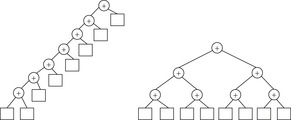
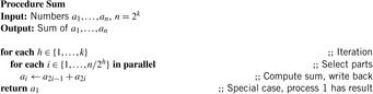
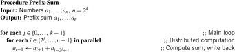
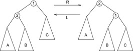
As an illustrative example for a parallel algorithm, consider the problem of adding eight numbers a1, …, a8. One option is to compute a1 + (a2 + (a3 + (a4 + (a5 + (a6 + (a7 + a8)))))) in a sequence. Obviously seven additions are necessary. Alternatively, we may add the numbers as (((a1 + a2) + (a3 + a4)) + ((a5 + a6) + (a7 + a8))). The corresponding trees are shown in Figure 9.1. The second sequence can be computed more efficiently in parallel if more than one process is available. If we have four processes only three parallel steps are necessary. In general, we have reduced the (parallel) running time from O(n) to O(lg n) by using n/2 processes. The procedure for the single process i is depicted in Algorithm 9.1. Each processor executes the loop O(lg n) times. The variables h, x, and y are local for each process. The algorithm is correct if the process works in lock-step mode, meaning that they execute the same steps at the same time. An example for the computation is provided in Figure 9.2.
One prominent computational model to analyze parallel algorithms is the parallel random access machine (PRAM). A PRAM has p processes, each equipped with some local memory. Additionally, all processes can access shared memory in which each process can directly access all memory cells. This is a coarse approximation of the most commonly used computer architectures. It concentrates on the partitioning of parts of computation and guarantees that data are present at the right point in time. The PRAM is programmed with a simple program that is parameterized with the process ID. A step in the execution consists of three parts: reading, calculating, and writing. A schematic view on a PRAM is shown in Figure 9.3.

To measure the performance of PRAM algorithms with respect to a problem of size n, the number of processes is denoted with p(n) and the parallel running time with tp(n), such that the total work is wp(n) = p(n) ⋅ tp(n). In a good parallelization the work of the parallel algorithm matches the time complexity t(n) of the sequential one. Since this is rarely the case, the term t(n)/wp(n) denotes the efficiency of the parallel algorithm. Sometimes a parallel algorithm is called efficient if for some constants k, k′ we have tp(n) = O(lgk t(n)) and wp(n) = O(t(n) lgk′ n), by means that the time is reduced to a logarithmic term and the work is only a logarithmic factor from the minimum possible. The speedup is defined as O(t(n)tp(n)), and is called linear in the number of processes, if p = O(t(n)/tp(n)). In rare cases, due to additional benefits of the parallelization, super-linear speedups can be obtained.
For our example problem of computing the sum of n numbers procedure Sum is efficient, as t(n = O(n) and tp(n) = O(lg n). However, the work for the p(n) = O(n) processors is wp(n) = O(n lg n), which is not optimal. A work-optimal algorithm for adding n numbers has two steps. In step 1 only n/lg n processors are used and lg n numbers are assigned to each processor. Each processor then adds lg n numbers sequentially in O(lg n) time. In step 2 there are n/lg n numbers left and we execute our original algorithm on these n/lg n numbers. Now we have tp(n) = O(lg n) and wp(n) = O(n).
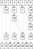
Using parallel computation it is possible to compute not only the final result sn = a1 + ⋯ + an but also all prefix sums (or partial sums) of the elements, namely all values sj = a1 + ⋯ + aj, 1 ≤ j ≤ n. The idea is to add all pairs of elements in parallel to produce n/21 sums, then add all pairs of those sums in parallel to produce n/22 sums, then add all pairs of those sums in parallel to produce n/23 sums, and so on. An implementation for such parallel scan computing of all prefix sums is provided in Algorithm 9.2 and an example of the application of the algorithm is given in Figure 9.4. Algorithm 9.2 is efficient, as tp(n) = O(lg n), but the work is O(n lg n). Fortunately, this can be reduced to wp(n) = O(n) (see Exercises).
 |
| Figure 9.4 |
The prefix sum algorithm has been applied as a subroutine in many parallel algorithms. For example, it helps to efficiently compress a sparse array or linked list or to simulate a finite-state machine (see Exercises).
Other basic building blocks for parallel algorithms are list ranking (compute distances of each element to the end of the list), matrix multiplication, and Euler tours (compute edge-disjoint cycles traversing all nodes). Fundamental PRAM algorithms include parallel merging and parallel sorting, parallel expression evaluation, and parallel string matching. Similar to the NP-completeness theory there is a theory on P-complete problems, which are sequentially simple but not parallel efficient. One representative problem in that class is the Circuit Value Problem: Given a circuit, the inputs to the circuit, and one gate in the circuit, calculate the output of that gate.
9.1.1. Motivation for Practical Parallel Search
For an early practical example of parallel state space search, we reconsider computing the most difficult problem instances for the Fifteen-Puzzle in two stages. First, a candidate set is determined, which contains all positions that require more than k moves (and some positions requiring less than k moves) using some upper-bound function. Then, for each candidate, iterative-deepening search using the Manhattan distance heuristic is applied to show that it can be excluded from the candidate set, or that it requires more than k moves.
The candidate set is generated by applying an upper-bound function U to all positions u in the Fifteen-Puzzle. Whenever U(u) > k, u becomes a candidate. The requirements on U are that it is fast to compute, so that it can be evaluated for all 1013 positions, and that it is a good upper-bound, so that the candidate set does not contain too many simple candidates. A first pattern database stores the optimal goal distances for all permutations of a subset of tiles. In the second step, the remaining tiles are moved to their goal location without moving the tiles fixed in the first step. A second pattern database contains the optimal goal distances for all permutations of the remaining tiles on the remaining board.
The obvious approach of actually solving each candidate requires too much time. For reducing the candidate set consistency constraints are applied. As an example, let u be a candidate and v its successor. If min{U(v) | v ∈ Succ(u)} < U(u) − 1, a shorter path for u can be found. Both steps of the algorithm are computationally expensive.
After applying consistency constraints, the following candidate set for k = 79 can be computed in parallel: U = 80, number of candidates 33,208; U = 81, number of candidates 1,339; and U = 82, number of candidates 44. The remaining 1,383 candidates with 81 or more moves can be solved in parallel. A bounded-depth macro move generator avoids repeating positions in shallow levels of the search tree (reducing the number of nodes in the very large search trees by roughly a factor of 4). The computation shows that all 1,383 candidates require less than 81 moves. Moreover, six positions require exactly 80 moves, for example, (15, 14, 13, 12, 10, 11, 8, 9, 2, 6, 5, 1, 3, 7, 4, 0). Therefore, this parallel computation proves that the hardest Fifteen-Puzzle positions require 80 moves to be solved.
The lesson to be learned is that for practical parallel search, traditional PRAM techniques are not sufficient to solve hard problems; refined engineering is needed.
9.1.2. Space Partitioning
Another outcome of this case study is that parallel duplicate detection is a challenge. It can lead to large communication overhead and, in some cases, considerable waiting times. What is needed is a projection of the search space onto the processing elements that maps successors of nodes to the same or a nearby process.
An important step is the choice of a suitable partition function to evenly distribute the search space over the processes. One option is a hash-based distribution with a hash function defined on the state vector. A hash-based distribution is effective if with high probability the successors of a state expanded at a particular process also map to the process. This results in low communication overhead.
The independence ratio measures how many nodes on average can be generated and processed locally. If it is equal to 1 all successors must be communicated. The larger the ratio, the better the distributed algorithm. Given 100 processors and a randomized distribution of successors, the ratio is 1.01, close to the worst case. A state space partitioning function should achieve two objectives: a roughly equal distribution of work on all processing units and a large independence ratio.
For large states full state hashing can become computationally expensive. As one solution to the problem, incremental hashing exploits the hash value difference between a state and its successors (see Ch. 3). Another approach is partial state hashing, truncates the state vector before computing the hash function and restricts to those parts that are changed least frequently.
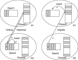
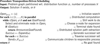
Transposition-driven scheduling is a solution that integrates asynchronous search with distributed hash tables for duplicate detection. The address returned by the hash function refers to both the process number and the local hash table. Rather than waiting for a result if a successor of an expanded node does not reside in the same process, the generated node is migrated to the destination process Pi. The latter one searches the node in the local table Closedi and stores the node in its work queue Openi. To reduce communication, several nodes with the same source and destination process are bundled into packages.
Figure 9.5 illustrates the main differences to distributed response strategies, where the result of the table lookup is communicated through the network. In contrast, transposition-driven scheduling includes the successor v of node u into the local work queue. This eases asynchronous behavior, since process P2 no longer has to wait for the response of process P1.
All processes are synchronized after all nodes for a given search threshold have been exhausted. The algorithm achieves the goal of preventing duplicate searches with local transposition tables. It has the advantage that all communication is asynchronous (nonblocking). No separate load balancing strategy is required; it is implicitly determined by the hash function.
Transposition-driven scheduling applies to general state space search. In the pseudo code of Algorithm 9.3 we show how a node is expanded and how its successors are sent to the neighbor based on the partitioning of the search space.
9.1.3. Depth Slicing
One drawback of static load balancing via fixed partition functions is that the partitioning may yield different search efforts in different levels of the search tree, so that processes far from the root will encounter frequent idling. Subsequent efforts for load balancing can raise considerable especially for small- and medium-size problems.
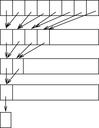
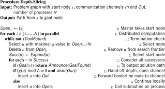
A dynamic partitioning method suitable for shared memory environments is depth-slicing. The rationale behind it is that if a hash-based partition function is used, there is a high probability that the successor states will not be handled by the node that generated them, resulting in a high network overhead. Roughly speaking, depth-slicing horizontally slices the depth-first search tree and assigns each slice to a different node. For the sake of simplicity, let us assume a unit cost state space, where we have access to the local depth d of every generated node. Each process decides to communicate a successor if d(u) exceeds a bound L. When a node is transmitted, the target processing unit will generate the search space with a newly initialized stack. The local depth will be initialized to zero. If the depth exceeds L again, it will be transmitted. The effect of this procedure will be a set of horizontal splits of the search tree (see Fig. 9.6). In every L level, states are transmitted from one process to the other. This induces that at about every d mod L steps, a state will be transferred. As a result, the independence ratio is close to L. If no hand-off is available, the process continues with its exploration. Since all processes are busy by then, the load is balanced.

Because only one stack on each process is available, the remaining question for the implementation (shown in Alg. 9.4) is when to select a node from the incoming queue, and when to select a node from the local stack. If incoming nodes are preferred, then the search may continue breadth-first instead of depth-first. On the other hand, if a node on the local stack is preferred, then a process would not leave its part of the tree. The solution is to maintain all nodes in a g-value-ordered list in which the local and communicated successors are inserted. For each expansion, the node with the maximum g-value is preferred. In the code, subindex i refers to the client process Pi that executes the code. The process P1 often takes a special role in initializing, finalizing, and coordinating the work among the processes, and is called the master.
Similar to horizontal depth-slicing a vertical partitioning of the search tree can be based on the heuristic values. The motivation for load balancing is that the expected distance to the goal (used here) is a similar measure compared to the distance to the start state (used in the previous method). The core advantage is that it is not only suited to depth-first but any general state expanding strategy.
9.1.4. Lock-Free Hashing
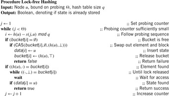
Lock-free algorithms guarantee systemwide progress in a concurrent environment of several running processing threads. The key is that modern CPUs implement an atomic compare-and-swap operation (CAS), so that always some thread can continue its work. For duplicate detection in state space search with a multicore CPU we require a lock-free hash table.
In this setting, however, we can only provide statistical progress guarantees and avoid explicit locks by CAS, which leads to a simpler implementation at no (visible) penalty in performance.
Strictly speaking, a lock-free hash algorithm in state space search locks in-place—it needs no additional variables for implementing the locking mechanism. CAS ensures atomic memory modification while preserving data consistency. This can be done by reading the value from memory, performing the desired computation on it, and writing the result back.
The problem with lock-free hashing is that it relies on low-level CAS operations with an upper limit on the data size that can be stored (one memory cell). To store state vectors that usually exceed the size of a memory cell, we need two arrays: the bucket and the data array.
Buckets store memorized hashes and the write status bit of the data in the data array. If h is the memorized hash, the possible values of the buckets are thus: (⋅, ⊤) for being empty, (h, ⊥) for being blocked for writing, and (h, ⊤) for releasing the lock. In the bucket the locking mechanism is realized by CAS. The specialized value (⊥) is a bitvector that indicates that the cell is used for writing. In the other cells the hash values are labeled unblocked. In a second background hash table data the states themselves are stored. A pseudo-code implementation is provided in Algorithm 9.5.
9.2. Parallel Depth-First Search
In this section we consider parallel depth-first search both in a synchronous and in an asynchronous setting, a notation that refers to the exchange of exploration information (nodes to expand, duplicates to eliminate) among different (depth-first) search processes. We also consider parallel IDA*–inspired search and algorithmic refinements like stack splitting and parallel window search.
Parallel depth-first search is often used synonymously to parallel branch-and-bound. For iterative-deepening search we distinguish between a synchronous and an asynchronous distribution. In the first case, work is distributed only within one iteration, and in the second case a process seeks work also within the next iteration. Therefore, asynchronous versions of IDA* are not optimal for the first solution found.
9.2.1. *Parallel Branch-and-Bound
Recall that a branch-and-bound algorithm consists of a branching rule that defines how to generate successors, a bounding rule that defines how to compute a bound, and an elimination rule that recognizes and eliminates subproblems, which cannot result in an optimal solution. In sequential depth-first branch-and-bound, a heuristic function governs the order in which the subproblems are branched from, and in case of being admissible it also defines the elimination rule. Different selections or bounding lead to different search trees.
The main difference between parallel implementations of branch-and-bound lies in the way information about the search process is shared. It consists of the states already generated, the lower bounds of the optimal solutions, and the upper bounds established. If the underlying state space is a graph, duplicate elimination is essential. Other parameters are the way that information is used in the individual processes, and the way it is divided.
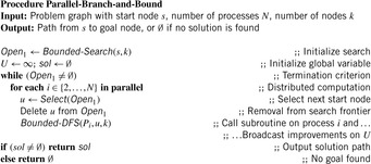
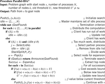
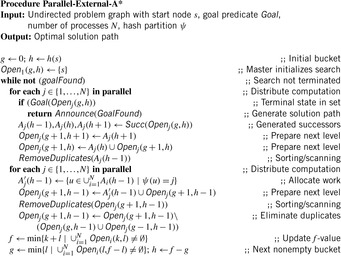
In the following we present a simple generic high-level asynchronous branch-and-bound algorithm. Every process stores the cost of the best solutions and broadcasts every improvement to the other processes, which in turn use the information on the global best solution cost for pruning.
Algorithm 9.6 shows a prototypical implementation. Like in the corresponding sequential version (see Alg. 5.3), U denotes a global upper bound, and sol the best solution found so far. Subroutine Bounded-DFS is called for individual searches on process Pi. The procedure works in the same way as Algorithm 5.4. It updates U and sol; the only difference is that the search is aborted if resources are exceeded. That is, the additional input variable k indicates that based on existing resources in time and space the work on each process is limited to a set of k-generated nodes. For the sake of simplicity we assume that the value is uniform for each participating process. In practice, this value can vary a lot, depending on the distribution of computational resources. We further assume that the sizes for the set of states for the master and the subprocesses are the same. In practice, the initial search tree and the subtree sizes have to be adjusted individually.
If within the given resource bound the search cannot be completed, value k can be increased to start a new run. Alternatively, the master's search frontier can be extended. Up to the communication of bounds and according solutions, the implementation of bounded DFS is equal to the sequential one. A real implementation depends on how information is exchanged: via files in a shared memory architecture, or via network communication in a cluster.
9.2.2. Stack Splitting
The parallel depth-first variant that we consider next is a task attraction scheme that shares subtrees among the processes on demand. This scheme works for depth-first search (see Alg. 9.7) but here we concentrate on iterative-deepening search.
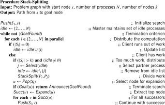
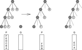
In the denotation derived earlier we consider a synchronous search approach that performs stack splits to explicit transfer nodes, where a stack split divides a larger stack of pending nodes to be expanded into pieces that can be distributed among available idle processes. In parallel stack-splitting search, each process works on its own local stack of frontier nodes. When the local stack is empty, a process issues a work request to another process. The donor then splits its stack and sends a part of its own work to the requester. Figure 9.7 illustrates the approach for two stacks P and Q, where the stack of requester Q is initially empty and the stack of donor P is split.
 |
| Figure 9.7 |
Initially, all work is given to the master. The other processes start with an empty stack, immediately asking for work. If the master has generated enough nodes, it splits its stack, donating subtrees to the requesting process.
There are several possible splitting strategies. If the search space is irregular, then picking half the states above the cutoff depth as in Figure 9.7 is appropriate. However, if strong heuristics are available, picking a few nodes closer to the threshold is recommended.
9.2.3. Parallel IDA*
For parallel heuristic search, sequential IDA* is an appropriate candidate to distribute, since it shares many algorithmic features with depth-first branch-and-bound. In contrast to A*, it can run with no or limited duplicate detection.
For a selected set of sliding-tile problems, parallel IDA* with stack splitting achieves almost linear speedups. These favorable results, however, apply only for systems with small communication diameters, like a hypercube, or a butterfly architecture. The identified bottleneck for massively parallel systems is that it takes a long time to equally distribute the initial workload, and that recursive stack splitting generates work packets with rather unpredictable processing times per packet. Moreover, the stack-splitting method requires implementation of explicit stack handling routines, which can be involved. A possible implementation for parallel IDA* with global synchronization is indicated in Algorithm 9.8.
In parallel window search, each process is given a different IDA* search threshold. In other words, we give different processes different estimates of the depth of the goal. In this way, parallelization cuts off many iterations of wrong guesses. All processes traverse the same search tree, but with different cost thresholds simultaneously. If a process completes an iteration without finding a solution it is given a new threshold. Some processes may consider the search tree with a threshold that is larger than others.
The advantage of parallel window search is that the redundant search inherent in IDA* is not performed serially. Another advantage of parallel window search is if the problem graph contains a larger density of goal nodes. Some processes may find an early solution in the search tree given a larger threshold while the others are still working on the smaller thresholds. A pseudo-code implementation is provided in Algorithm 9.9. Since sequential IDA* stops searching after using the right search bound, parallel window search can result in a large number of wasted node expansions.
The two ideas of parallel window search and node ordering have been combined to eliminate the weaknesses of each approach while retaining their strengths. In ordinary IDA* search, children are expanded in a depth-first manner from left to right, bounded in depth by the cost threshold. In parallel window search, the search algorithm expands the tree a few levels and sorts the search frontier by increasing h-value. This frontier set is updated for each iteration. Nodes with smaller h-values are preferred. The resulting merge finds near-optimal solutions quickly, improves the solution until it is optimal, and then finally guarantees optimality, depending on the amount of time available.
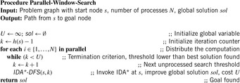
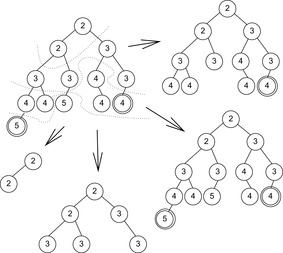
An example on how search tree nodes are spread among different processes is provided in Figure 9.8. We see that the process with threshold 5 can find a suboptimal solution earlier than one that searches with optimal threshold 4.
9.2.4. Asynchronous IDA*
A generic scheme for highly parallel iterative-deepening search on asynchronous systems is asynchronous IDA*. The algorithm is based on a data partitioning, where different parts of the search space are processed asynchronously by sequential routines running in parallel on the distributed processing elements. The algorithm consists of three phases:
• Data Partitioning: All processes redundantly expand the first few tree levels until a sufficient amount of nodes is generated.
• Distribution: Each process selects some nodes from the frontier nodes of the first phase for further expansion. One way of obtaining a widespread distribution of nodes is to assign nodes i, p + i, …, k ⋅ p + i to process i. The nodes are expanded to produce a larger set of, say, some thousand fine-grained work packets for the subsequent asynchronous search phase.
• Asynchronous Search: The processes generate and explore different subtrees in an iterative-deepening manner until one or all solutions are found. Since the number of expanded nodes in each work package usually varies and is not known in advance, dynamic load balancing is needed.
None of these three phases requires a hard synchronization. Processors are allowed to proceed with the next phase as soon as they finished the previous one. Only in the third phase, some mechanism is needed to keep all processes working on about the same search iteration. However, this synchronization is a weak one. If a process runs out of work, it requests unsolved work packages from a designated neighborhood (the original algorithm was run on a transputer system, where processors are connected in a two-dimensional grid structure). If such a package is found, its ownership is transferred to the previously idle processor. Otherwise, it is allowed to proceed with the next iteration. Load balancing ensures that all processors finish their iterations at about the same time.
9.3. Parallel Best-First Search Algorithms
At first glance, best-first search is more difficult to parallelize than IDA*. The challenge lies in the distributed management of the Open and Closed lists. It is no longer guaranteed that the first goal is optimal. It can happen that the optimal solution is computed by some other process such that a global termination criterion has to be established. One nonadmissible solution is to accept a goal node that has been found by one process only if no other process has a better f-valued node to expand.
From the host of different suggestions we exemplarily selected one global approach that takes shared memory and flexible data structures to rotate locks down a tree. For local A* search that is based on a hash partitioning of the search space, different load balancing and pruning strategies are discussed.
9.3.1. Parallel Global A*
A simple parallelization of A*, called parallel global A*, follows an asynchronous concurrent scheme. It lets all available processes work in parallel on one node at a time, accessing data structures Open and Closed that are stored in global, shared memory. As opposed to that,parallel local A* (PLA*) uses data structures local to each process; they are discussed in the next section.
The advantage of parallel global A* is that it provides small search overheads, because especially in a multiprocessor environment with shared memory, global information is available for all processors. However, it also introduces difficulties. Since the two lists Open and Closed are accessed asynchronously, we have to choose data structures that ensure consistency for efficient parallel search.
If several processes wish to extract a node from Open and modify the data structure, consistency can only be guaranteed by granting mutually exclusive access rights or locks. In addition, if the Closed structure is realized by storing pointers to nodes in Open, it too would have to be partially locked. These locks reserialize parts of the algorithm and can limit the speedup.
*Treaps
One proposal is to use a priority search tree data structure, called a treap, to represent Open and Closed jointly. This saves the effort of having to manage two separate data structures.
Treaps exhibit the properties of binary search trees and heaps (see Ch. 3) at the same time. Let X be a set of n items, associated both with a key and a priority. Keys and priorities come from two ordered universes that need not be the same. A treap for X is a binary tree with node set X that is arranged such that the priorities satisfy the heap property and, as in an ordinary search tree, the keys are sorted in an in-order traversal. More precisely, the following invariants hold for nodes u and v:
• If v is a left child of u, then key(v) < key(u).
• If v is a right child of u, then key(v) > key(u).
• If v is a child of u, then priority(v) > priority(u).
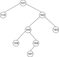
It is easy to see that for any set X a treap exists and that by the heap property of the priorities the item with the smallest priority is located at the root. To construct a treap for X from scratch (assuming that the key is unique), we first select the element x ∈ X with the smallest priority. Then, we partition X into X′ = {y ∈ X | key(y) < key(x)} and X″ = {y ∈ X | key(y) > key(x)} and construct the treaps for the sets X′ and X″ recursively, until we reach a singleton set that corresponds to a leaf. Figure 9.9 shows a treap for the set of (priority, key)-pairs {(11, 4), (12, 1), (13, 8), (14, 5), (15, 7), (16, 6), (18, 2), (19, 3)}.
 |
| Figure 9.9 |
The access operations on a treap T are as follows. Lookup(key) finds the item x in T with matching key using the binary tree search. Insert(x) adds the item x to T. Let y be an item already in T with matching key. If the priority of y is smaller than the one of x then x is not inserted; otherwise, y is removed and x is inserted. DeleteMin selects and removes the item x with the smallest priority and Delete(x) removes the item x from T.
Insertion makes use of the subtree rotation operation, an operation known from other (balanced) binary search tree implementations (see Fig. 9.10). First, using the key of x we search the position with respect to the in- and heap-ordering among the nodes. The search stops when an item y is found with a priority larger than the one of x, or an item z is encountered with the matching key component. In the first case, the item x is inserted between y and the parent of y. In the second case, x must not be inserted in the treap since the priority of x is known to be larger than the one of z. In the modified tree all nodes are in heap-order. To reestablish the in-order, the splay operation is needed that splits the subtree rooted at x into two parts: one with the nodes that have a key smaller than x and one with the nodes that have a key larger than x. All nodes y that turn out to have the same key component during the splay operation are deleted. The splay operation is implemented using a sequence of rotations.
The operations Delete and DeleteMin are similar in structure. Both rotate x down until it becomes a leaf, where it can be deleted for good. The time complexity for each of the operations is proportional to the depth of the treap, which can be linear in the worst case but remains logarithmic for random priorities.
*Locking
Using a treap the need for exclusive locks can be alleviated to some extent. Each operation on the treap manipulates the data structure in the same top-down direction. Moreover, it can be decomposed into successive elementary operations. The tree partial locking protocol uses the paradigm of user view serialization. Every process holds exclusive access to a sliding window of nodes in the tree. It can move this window down a path in the tree, which allows other processes to access different, nonoverlapping windows at the same time.
Parallel A* using a treap with partial locking has been tested for the Fifteen-Puzzle on different architectures, with a speedup for eight processors in between 2 and 5.
9.3.2. Parallel Local A*
In parallel local A*, each process is allocated a different portion of the search space represented in its own local data structures. In this case, the inconsistencies of multiple lists introduce a number of inefficiencies. Processes run out of work and become idle. Since processes perform local rather than global best-first search, many processes may expand nonessential nodes, additionally causing a memory overhead. In a state space search graph duplicates arise in different processes, so that load balancing is needed to minimize nonessential work and pruning strategies to avoid duplicate work.
Different solutions for load balancing have been proposed. Earlier approaches use either quantitative balancing strategies like round-and-robin and neighborhood averaging, or qualitative strategies like random communication, AC, and LM. In round-and-robin, a process that runs out of work requests work from its busy neighbors in a circular fashion. In neighborhood averaging, the number of active nodes among the neighboring processors are averaged. In random communication, each processor donates the newly generated children generated in each iteration to a random neighbor. In the AC and LM strategies, each processor periodically reports the nondecreasing list of costs of nodes in Open to its neighbors, and computes its relative load to decide which nodes to transfer. One compromise between quantitative and qualitative load balancing is quality equalizing, in which processors utilize load information of neighboring processes to balance the load via nearest-neighbor work transfers. In summary, most load balancing schemes transfer work from a donor processor to an acceptor processor.
There are two essentially different strategies for pruning: global and local hashing. For global hashing, for example, multiplicative hash functions (Ch. 3) apply. By using the hash function also to balance the load, all duplicates will be hashed to the same process and can be eliminated. As a drawback, transmissions for duplicate pruning are global and increase message latency. In local hashing a search space partition scheme is needed. This ensures that any set of duplicate nodes arises only within a particular process group. Finding suitable local hash functions is a domain-dependent task and is sensible to the parallel architecture. Design principles that have been exploited are graph leveling, clustering, and folding. State space graph leveling applies to many combinatorial optimization problems, and every search node has a unique level. In clustering, the effect on the throughput requirements of duplicate pruning is analyzed, while folding is meant to achieve static load balance across parallel hardware substructures. Speedups obtained for global hashing are better than without hashing, but often smaller than for local hashing. In both cases, quality equalizing improves the speedup substantially.
The number of generated nodes in parallel A* search can grow quickly, so that strategies for searching with restricted or fixed amount of memory may become necessary. In this case, we apply memory-restricted search algorithms (see Ch. 6) extended to the situation, where main memory, even if shared among different processors, becomes rare. Partial expansion is one of the best choices to improve the performance of A* processes that run in parallel.
9.4. Parallel External Search
Good parallel and I/O-efficient designs have much in common. Moreover, large-scale parallel analyses often exceed main memory capacities. Hence, combined parallel and external search executes an external memory exploration (see Ch. 8) in distributed environments like multiprocessor machines and workstation clusters. One main advantage is that duplicate detection can often be parallelized from avoiding concurrent writes.
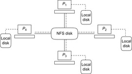
In similarity to the parallel memory model of a PRAM the distributed memory model by Vitter and Shriver is a PDISK model. Each processor has its own local hard disk and the processes communicate with each other via the network and access a global hard disk (see Fig. 9.11).
As with the PRAM model, complexity analyses do not always map to practical performance, since either the disk transfer or the internal calculations can become the computational bottleneck.
In this section we first consider parallel external BFS with delayed, hash-based duplicate detection in the example of completely exploring the Fifteen-Puzzle. Next, we consider parallelizing structured duplicate detection with a partitioning based on abstract state spaces, and parallel external A* with a partitioning based on g-values and h-values. We close the section with the parallel and disk-based computation of heuristic values based on selected patterns and corresponding distributed (possibly additive) databases.
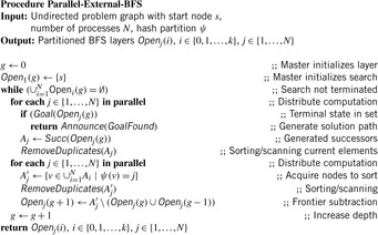
9.4.1. Parallel External Breadth-First Search
In parallel external breadth-first search with delayed duplicate detection, the state space is partitioned into different files using a global hash function to distribute and locate states. For example, in state spaces like the Fifteen-Puzzle that are regular permutation games, each node can be perfectly hashed to a unique index, and some prefix of the state vector can be used for partitioning. Recall that if state spaces are undirected, frontier search (see Sec. 6.3.3, p. 257) can distinguish neighboring nodes that have already been explored from those that have not, and, in turn, omit the Closed list.
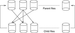
Figure 9.12 depicts the layered exploration on the external partition of the state space with a hash function that partitions both the current parent layer and the child layer for the successors into files. If a layer is done, child files are renamed into parent files to iterate the exploration.
It turned out that even on a single processor, multiple threads maximize the performance of the disks. The reason is that a single-threaded implementation will block until the read from or write to disk has been completed.
Hash-based delayed duplicate detection on the state vector prefix works well to generate a suitable partition for the Fifteen-Puzzle. Within one iteration, most file accesses can be performed independently. The two processes will be in conflict only if we simultaneously expand two parent files that have a child file in common.
To realize parallel processing a work queue is maintained, which contains parent files waiting to be expanded and child files waiting to be merged. At the start of each iteration, the queue is initialized to contain all parent files. Once all parents of a child file are expanded, the child file is inserted into the queue for early merging.
Each process works as follows. It first locks the work queue. The algorithm checks whether the first parent file conflicts with any other file expansion. If so, it scans the queue for a parent file with no conflicts. It swaps the position of that file with the one at the head of the queue, grabs the nonconflicting file, unlocks the queue, and expands the file. For each file it generates, it checks if all of its parents have been expanded. If so, it puts the child file at the head of the queue for expansion, and then returns to the queue for more work. If there is no more work in the queue, any idle process waits for the current iteration to complete. At the end of each iteration the work queue is reinitialized to contain all parent files for the next iteration. Algorithm 9.10 shows a pseudo-code implementation. Figure 9.13 illustrates the distribution of a bucket among three processors.
A complete search for the Fifteen-Puzzle with its 16!/2 states has been executed using a maximum of 1.4 terabytes of disk storage. Three parallel threads on two processors completed the search in about four weeks. The results are shown in Table 9.1 and validate that the diameter of the Fifteen-Puzzle is 80.
9.4.2. Parallel Structured Duplicate Detection
Structured duplicate detection (Ch. 6) performs early duplicate detection in the RAM. Each abstract state represents a file containing every concrete state mapping to it. Since all adjacent abstract states were loaded into main memory, duplicate detection for concrete successor states remains in the RAM.
We assume breadth-first heuristic search as the underlying search algorithm (see Ch. 6), which generates the search space with increasing depth, but prunes it with respect to the f-value, provided that the optimal solution length is known. If not, external A* or iterative-deepening breadth-first heuristic search applies.
Structured duplicate detection extends nicely to a parallel implementation. In parallel structured duplicate detection abstract states together with their abstract neighbors are assigned to a process. We assume that the parallelization takes care of synchronization after one breadth-first search iteration has been completed, because a concurrent expansion in different depths likely affects the algorithm's optimality.
If in one BFS level two abstract nodes together with their successor do not overlap, their expansion can be executed fully independently on different processors. More formally, let ϕ(u1) and ϕ(u2) be the two abstract nodes; then the scopes of ϕ(u1) and ϕ(u2) are disjoint if  . This parallelization maintains locks only for the abstract space. No locks for individual states are needed.
The approach applies to both shared and distributed memory architectures. In the shared implementation each processor has a private memory pool. As soon as this is exhausted it asks the master process (that has spawned it as a child process) for more memory that might have been released using a completed exploration by some other process.
For a proper (conflict-free) distribution of work for undirected search spaces, numbers I(ϕ(u)) were assigned to each abstract node ϕ(u), denoting the accumulated influence that currently is imposed to this node by running processes. If I(ϕ(u)) = 0 the abstract node ϕ(u) can be picked for expansion from every processor that is currently idle. Function I is updated as follows. In a first step, for all ϕ(v) ≠ ϕ(u) with ϕ(u) ∈ Succ(ϕ(v)) value ϕ(v) is incremented by one: All abstract nodes that include ϕ(u) in their scope cannot be expanded, since ϕ(u) is chosen for expansion. In a second step, for all ϕ(v) ≠ ϕ(u) with ϕ(v) ∈ Succ(ϕ(u)) and all ϕ(w) ≠ ϕ(v) with ϕ(w) ∈ Succ(ϕ(v)) value ϕ(v) is incremented by one: All abstract nodes that include any ϕ(v) as a successor of ϕ(u) cannot be expanded, since they are also assigned to the processor.
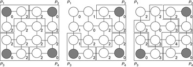
Figure 9.14 illustrates the working of parallel structural duplicate detection for the Fifteen-Puzzle with the currently expanded abstract nodes shaded. The left-most part of the figure shows the abstract problem graph together with four processes working independently at expanding abstract states. The numbers I(ϕ(u)) are associated with each abstract node ϕ(u). The middle part of the figure depicts the situation after one process has finished, and the right part shows the situation after the process has been assigned to a new abstract state.
9.4.3. Parallel External A*
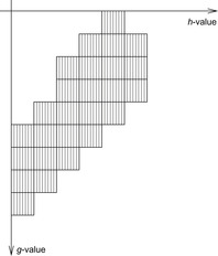
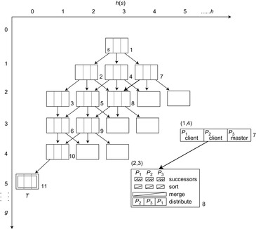
The distributed version of external A*, called parallel external A*, is based on the observation that the internal work in each individual bucket of external A* can be parallelized among different processes. More precisely, each two states in a bucket Open(g, h) can be expanded in different processes at the same time. An illustration is given in Figure 9.15, indicating a uniform partition available for each Open(g, h)-bucket. We discuss disk-based message queues to distribute the load among different processes.
 |
| Figure 9.15 |
Disk-Based Queues
To organize the communication between the processes a work queue is maintained on disk. The work queue contains the requests for exploring parts of a (g, h)-bucket together with the part of the file that has to be considered. (Since processes may have different computational power and processes can dynamically join and leave the exploration, the size of the state space partition does not necessarily have to match the number of processes. By utilizing a queue, we also may expect a process to access a bucket multiple times. However, for the ease of a first understanding, it is simpler to assume that the jobs are distributed uniformly among the processes.) For improving the efficiency, we assume a distributed environment with one master and several client processes. In the implementation, the master is in fact an ordinary process defined as the one that finalized the work for a bucket. This applies to both the cases when each client has its own hard disk or if they work together on one hard disk (e.g., residing on the master). We do not expect all processes to run on one machine, but allow clients to log on the master machine, suitable for workstation clusters. Message passing between the master and client processes is purely done on files, so that all processes are fully autonomous. Even if client processes are killed, their work can be redone by any other idle process that is available.
One file, which we call the expand-queue, contains all current requests for exploring a node set that is contained in a file (see Fig. 9.16). The filename consists of the current g-values and h-values. In case of larger files, file pointers for processing parts of a file are provided to allow for better load balancing. There are different strategies to split a file into equidistance parts, depending on the number and performance of logged-on clients. Since we want to keep the exploration process distributed, we select the file pointer windows into equidistant parts of a fixed number of C bytes for the nodes to be expanded. For improved I/O, the number C is supposed to divide the system's block size B. As concurrent read operations are allowed for most operating systems, multiple processes reading the same file impose no concurrency conflicts.
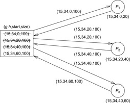
The expand-queue is generated by the master process and is initialized with the first block to be expanded. Additionally, we maintain the total number of requests, the size of the queue, and the current number of satisfied requests. Any logged-on client reads a request and increases the count once it finishes. During the expansion process, in a subdirectory indexed by the client's name it generates different files that are indexed by the g-values and h-values of the successor nodes.
The other queue is the refine-queue, which is also generated by the master process once all processes are done. It is organized in a similar fashion as the expand queue and allows clients to request work. The refine-queue contains filenames that have been generated above, namely the name of the client (that does not have to match with the one of the current process), the block number, and the g-values and h-values. For a suitable processing the master process will move the files from subdirectories indexed by the slave's name to ones that are indexed by the block number. Because this is a sequential operation executed by the master thread, changing the file locations is fast in practice.
To avoid redundant work, each process eliminates the requests from the queue. Moreover, after finishing the job, it writes an acknowledgment to an associated file, so that each process can access the current status of the exploration and determine if a bucket has been completely explored or sorted.
All communication between different processes can be realized via shared files so that a message passing unit is not required. However, a mechanism for mutual exclusion is necessary. A rather simple but efficient method to avoid concurrent writes accesses is the following. Whenever a process has to write on a shared file, it issues an operating system command to rename the file. If the command fails, it implies that the file is currently being used by another process.
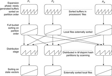
Sorting and Merging
For each bucket under consideration, we establish four stages in Algorithm 9.11. These stages are visualized in Figure 9.17 (top to bottom). Zig-zag curves illustrate the order of the nodes in the files with regard to the comparison function used. As the states are presorted in internal memory, every peak corresponds to a flushed buffer. The sorting criteria are defined first by the node's hash key and then by the low-level comparison based on the (compressed) state vector.
 |
| Figure 9.17 |
In the exploration stage (generating the first row in the figure), each process p flushes the successors with a particular g-value and h-value to its own file (g, h, p). Each process has its own hash table and eliminates some duplicates already in main memory. The hash table is based on chaining, with chains sorted along the node comparison function. However, if the output buffer exceeds memory capacity it writes the entire hash table to disk. By the use of the sorting criteria as given earlier, this can be done using a mere scan of the hash table.
In the first sorting stage (generating the second row in the figure), each process sorts its own file. In the distributed setting we exploit the advantage that the files can be sorted in parallel, reducing internal processing time. Moreover, the number of file pointers needed is restricted by the number of flushed buffers, and illustrated by the number of peaks in the figure. Based on this restriction, we only need a merge of different sorted buffers.
In the distribution stage (generating the third row in the figure), all nodes in the presorted files are distributed according to the hash value's range. As all input files are presorted this is a mere scan. No all-including file is generated, keeping the individual file sizes small. This stage can be a bottleneck to the parallel execution, as processes have to wait until the distribution stage is completed. However, if we expect the files to reside on different hard drives, traffic for file copying can be parallelized.
In the second sorting stage (generating the last row in the figure), processes resort the files (with buffers presorted wrt. the hash value's range) to find further duplicates. The number of peaks in each individual file is limited by the number of input files (= number of processes), and the number of output files is determined by the selected partitioning of the hash index range. Using the hash index as the sorting key we establish that the concatenation of files is sorted.
Figure 9.18 shows the distribution of states into buckets with three processors.
Complexity
The lower bound for the I/O complexity for delayed duplicate elimination in an implicit undirected unit-cost graph A* search with consistent estimates is Ω(sort(|E|)), where E is the set of explored edges in the search graph. Fewer I/Os can only be expected if structural properties can be exploited. But by assuming a sufficient number of file pointers, the external memory sorting complexity reduces to Ω(scan(|E|)) I/Os, since a constant number of merging iterations suffice to sort the file.
Strictly speaking, the total number of I/Os cannot be reduced by parallel search. More disks, however, reduce the number of I/Os; that is, scan(|E|) = O(|E|/DB. If the number of disks D equals the number of processes N then we can have a speedup of N either with local or global hard disk access. Using this we can achieve in fact a linear number of I/Os for delayed duplicate elimination and sorting.
An important observation is that the more processes we invest, the finer the partitioning of the state space, and the smaller the individual file sizes will be. Therefore, a side effect of having more processes at hand is an improvement in I/O performance.
9.4.4. Parallel Pattern Database Search
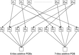
Disjoint pattern databases can be constructed embarrassingly parallel. The subsequent search, however, faces the problem of high memory consumption due to many large pattern databases, since loading pattern databases on demand significantly slows down the performance.
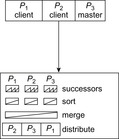
One solution is to distribute the lookup to multiple processes. For external A* this works as follows. As buckets are fully expanded, the order in a bucket does not matter, so we can distribute the work for expansion, evaluation, and duplicate elimination. For the Thirty-Five-Puzzle we choose one master to distribute generated states to 35 client processes Pi, each one responsible for one tile i for i ∈ {1, …, 35}. All client processes operate individually and communicate via shared files.
During the expansion of a bucket (see Fig. 9.19), the master writes a file Ti for each client process Pi, i ∈ {1, …, 35}. Once it has finished the expansion of a bucket, the master Pm announces that each Pi should start evaluating Ti. Additionally, the client is informed on the current g-value and h-value. After that, the master Pm is suspended, and waits for all Pi's to complete their task. To relieve the master from load, no sorting takes place during distribution. Next, the client processes start evaluating Ti, putting their results into Ei(h − 1) or Ei(h + 1), depending on the observed difference in the h-values. All files Ei are additionally sorted to eliminate duplicates, internally (when a buffer is flushed) and externally (for each generated buffer). Because only three buckets are opened at a time (one for reading and two for writing) the associated internal buffers can be large.
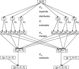
After the evaluation phase is completed, each process Pi is suspended. When all clients are done, the master Pm is resumed and merges the Ei(h − 1) and Ei(h + 1) files into Em(h − 1) and Em(h + 1). The merging preserves the order in the files Ei(h − 1) and Ei(h + 1), so that the files Em(h − 1) and Em(h + 1) are already sorted with all duplicates within the bucket eliminated. The subtraction of the bucket (g − 1, h − 1) from Em(h − 1) and (g − 1, h + 1) from Em(h + 1) now eliminates duplicates from the search using a parallel scan of both files.
Besides the potential for speeding up the evaluation, the chosen distribution mainly saves space. On one hand, the master process does not need any additional memory for loading pattern databases. It can invest all its available memory for internal buffers required for the distribution, merging, and subtraction of nodes. On the other hand, during the entire lifetime of client process Pi, it has to maintain only the pattern database Dj that includes tile i in its pattern (see Fig. 9.20).
9.5. Parallel Search on the GPU
In the last few years there has been a remarkable increase in the performance and capabilities of the graphics processing unit (GPU). Modern GPUs are not only powerful, but also parallel programmable processors featuring high arithmetic capabilities and memory bandwidths. High-level programming interfaces have been designed for using GPUs as ordinary computing devices. These efforts in general-purpose GPU programming (GPGPU) have positioned the GPU as a compelling alternative to traditional microprocessors in high-performance computing. The GPU's rapid increase in both programmability and capability has inspired researchers to map computationally demanding, complex problems to it. However, it is a challenge to effectively use these massively parallel processors to achieve efficiency and performance goals. This imposes restrictions on the programs that should be executed on GPUs.
Since the memory transfer between the card and main board on the express bus is extremely fast, GPUs have become an apparent candidate to speed up large-scale computations. In this section we consider the time-efficient generation of state spaces on the GPU, with state sets made available via a transfer from/to main and secondary memory. We start with describing typical aspects of an existing GPU. Algorithmically, the focus is on GPU-accelerated BFS, delayed duplicate detection, and state compression. We then look into GPU-accelerated bitvector breadth-first search. As an application domain, we chose the exploration in sliding-tile puzzles.
9.5.1. GPU Basics
GPUs are programmed through kernels that are selected as threads to run on each core, which is executed as a set of threads. Each thread of the kernel executes the same code. Threads of a kernel are grouped in blocks. Each block is uniquely identified by its index and each thread is uniquely identified by the index within its block. The dimensions of the thread and the thread block are specified at the time of launching the kernel.
Programming GPUs is facilitated by APIs and support special declarations to explicitly place variables in some of the memories (e.g., shared, global, local), predefined keywords (variables) containing the block and thread IDs, synchronization statements for cooperation between threads, runtime API for memory management (allocation, deallocation), and statements to launch functions on GPU. This minimizes the dependence of the software from the given hardware.
The memory model loosely maps to the program thread-block-kernel hierarchy. Each thread has its own on-chip registers, which are fast, and off-chip local memory, which is quite slow. Per block there is also an on-chip shared memory. Threads within a block cooperate via this memory. If more than one block is executed in parallel then the shared memory is equally split between them. All blocks and threads within them have access to the off-chip global memory at the speed of RAM. Global memory is mainly used for communication between the host and the kernel. Threads within a block can communicate also via lightweight synchronization.
GPUs have many cores, but the computational model is different from the one on the CPU. A core is a streaming processor with some floating point and arithmetic logic units. Together with some special function units, streaming processors are grouped together to form streaming multiprocessors (see Fig. 9.21).
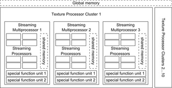
Programming a GPU requires a special compiler, which translates the code to native GPU instructions. The GPU architecture mimics a single instruction multiply data computer with the same instructions running on all processors. It supports different layers for accessing memory. GPUs forbid simultaneous writes to a memory cell but support concurrent reads.
On the GPU, memory is structured hierarchically, starting with the GPU's global memory called video RAM, or VRAM. Access to this memory is slow, but can be accelerated through coalescing, where adjacent accesses with less than word-width number bits are combined to full word-width access. Each streaming multiprocessor includes a small amount of memory called SRAM, which is shared between all streaming multiprocessors and can be accessed at the same speed as registers. Additional registers are also located in each streaming multiprocessor but not shared between streaming processors. Data have to be copied to the VRAM to be accessible by the threads.
9.5.2. GPU-Based Breadth-First Search
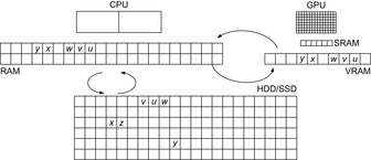
We assume a hierarchical GPU memory structure of SRAM (small, but fast and parallel access) and VRAM (large, but slow access). The general setting is displayed in Figure 9.22. In the following we illustrate how to perform GPU-based breadth-first search, generating the entire search space.
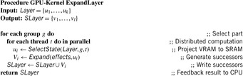
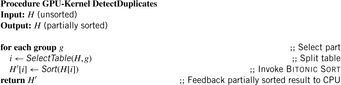
Algorithm 9.12 displays the main search algorithm running on the CPU. For each BFS level it divides into two computational parts that are executed on the GPU: applying actions to generate the set of successors, and detecting and eliminating duplicates in a delayed fashion via GPU-based sorting.
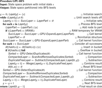
The two according kernel functions that are executed on the graphics card are displayed in Algorithm 9.13 and Algorithm 9.14. For the sake of clarity we haven't shown the transfer from hard disk to RAM and back for BFS-levels that do not fit in RAM, nor the copying from RAM to VRAM and from VRAM to the SRAM, as needed for GPU computation.
One example for the subtleties that arise is that for better compression in RAM and on disk, we keep the search frontier and the set of visited states distinct, since only the first one needs to be accessible in uncompressed form.
Delayed Duplicate Detection on the GPU
For delayed elimination of duplicates, we have to order a BFS level with regard to a comparison function that operates on states (sorting phase). The array is then scanned and duplicates are removed (compaction). Considering the strong set of assumptions of orthogonal, disjoint, and concise hash functions, ordinary hash-based delayed duplicate detection is often infeasible. Therefore, we propose a trade-off between sorting-based and hash-based delayed duplicate detection by sorting buckets that have been filled through applying a hash function. The objective is that hashing in RAM performs more costly distant data moves, while subsequent sorting addresses local changes, and can be executed on the GPU by choosing the bucket sizes appropriately. If the buckets fit into the SRAM, they can be processed in parallel.
Disk-based sorting refers to one of the major success stories for GPU computation. Various implementations have been proposed, including variants of Bitonic Sort and GPU-based Quicksort. Applying the algorithms to larger state vectors, however, fails as their movements within the VRAM slows down the computation significantly. Trying to sort an array of indexes also fails, since now the comparison operator exceeds the boundary of the SRAM. This leads to an alternative design of GPU sorting for state space search.
Hash-Based Partitioning
The first phase of sorting smaller blocks in Bitonic Sort is fast, but merging the presorted sequences for a total ordered slows down the performance. Therefore, we employ hash-based partitioning on the CPU to distribute the elements into buckets of adequate size (see Fig. 9.23). The state array to be sorted is scanned once. Using hash function h and a distribution of the VRAM into k blocks, the state s is written to the bucket with index h′(s) = h(s) mod k. If the distribution of the hash function is appropriate and the maximal bucket sizes are not too small, a first overflow occurs when the entire hash table is occupied to more than a half. All remaining elements are set to a predefined illegal state vector that realizes the largest possible value in the ordering of states.
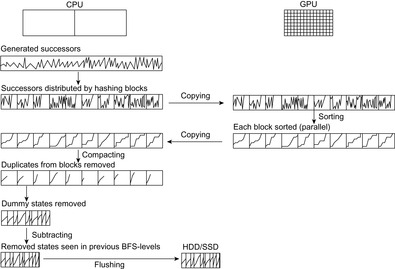
This hash-partitioned vector of states is copied to the graphics card and sorted by the first phase of Bitonic Sort. The crucial observation is that, due to the presorting, the array is not only partially sorted with regard to the comparison function operating on states s, but totally sorted with regard to the extended comparison function operating on the pairs (h′(s),s). The sorted vector is copied back from VRAM to RAM, and the array is compacted by eliminating duplicates with another scan through the elements. Subtracting visited states is made possible through scanning all previous BFS-levels residing on disk. Finally, we flush the duplicate-free file for the current BFS-level to disk and iterate. To accelerate discrimination and to obey the imposed order on disk, the hash bucket value h′(s) is added to the front of the state s.
If a BFS-level becomes too large to be sorted on the GPU, we split the search frontier into parts that fit in the VRAM. This yields some additional state vector files to be subtracted to obtain a duplicate-free BFS-level, but in practice, time performance is still dominated by expansion and sorting. For the case that subtraction becomes harder, we can exploit the hash partitioning, inserting previous states into files partitioned by the same hash value. States that have a matching hash value are mapped to the same file. Provided that the sorting order is defined first on the hash value then on the state vector itself, after the concatenation of files (even if sorted separately) we obtain a total order on the sets of states. This implies that we can restrict duplicate detection including subtraction to states that have matching hash values.
Instead of sorting the buckets after they have been filled, it is possible to use chaining right away, checking each individual successor for having a duplicate against the states stored in its bucket. Keeping the list of states sorted, as in ordered hashing, accelerates the search, but requires additional work for insertion and does not speed up the computation, if compared to parallel sorting the buckets on the GPU. A refinement checks the state to be inserted in a bucket with the top element to detect some duplicates quickly.
State Compression
With a 64-bit hash address collision even in very large state spaces are rare. Henceforth, given hash function h, we compress the state vector for u to (h(u), i(u)), where i(u) is the index of the state vector residing in RAM that is needed for expansion. We sort the pairs on the GPU with respect to the lexicographic ordering of h. The shorter the state vector, the more elements fit into one group, and the better the expected speedup on the GPU.
To estimate the error probability assume a state space of n = 230 elements uniformly hashed to the m = 264 possible bitvectors of length 64. According to the birthday problem, the probability of having no duplicates is m!/(mn(m − n)!). One known upper bound is e−n(n − 1)/2m, which in our case leads to a less than 96.92% chance of having no collision at all. But how much less can this be? For better confidence on our algorithm, we need a lower bound. We have For our case this resolves to a confidence of at least 93.94% that no duplicate arises while hashing the entire state space to 64 bits (per state). Recall that missing a duplicate harms, only if the missed state is the only way to reach the goal. If this confidence is too low, we may rerun the experiment with another independent hash function, certifying that with more than a 99.6% chance, the entire state space has been traversed.
Array Compaction
The compaction operation for sorted state sets can be accelerated on a parallel machine using an additional vector unique as follows. The vector is initialized with 1s, denoting that we initially assume that states are unique. In a parallel scan, we then compare a state with its left neighbor and mark the ones that are not unique by setting its entry to 0. Next, we compute the prefix sum to compute the final indices for compaction.
Duplicates in previous levels can be eliminated in parallel as follows. First we map as many BFS-levels as possible into the GPU. Processor pi scans the current BFS-level t and a selected previous layer i ∈ {0, …, t − 1}. As both arrays Open(t) and Open(i) are sorted, the time complexity for the parallel scan is acceptable, because the arrays have to be mapped from RAM to VRAM and back anyway. If a match is found, array unique is updated, setting the according bit in Opent to 0. The parallelization we obtain for level subtraction is due to processing different BFS levels, and for sorting and scanning due to partitioning the array. Because all processors read the array Opent we allow concurrent read. Additionally, we allow each processor to write into the array unique. Since previous layers are mutually disjoint, no processor will access the same position, so that the algorithm preserves exclusive writes.
Expansion on the GPU
The remaining bottleneck is the CPU performance in generating the successors, which can also be reduced by applying parallel computation. For this we port the expansion for states to the GPU, parallelizing the search.
For BFS, the order of expansions within one bucket does not matter, so that no communication between threads is required. Each processor simply takes its share and starts expanding. Having fixed the set of applicable actions for each state, generating the successors in parallel on the GPU is immediate by replicating each state to be expanded by the number of applicable actions. All generated states are copied back to RAM (or by directly applying the GPU sorting).
9.5.3. Bitvector GPU Search
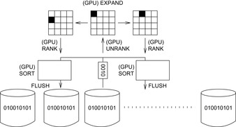
In the advent of perfect and inversible hash functions (see Ch. 3), a bitvector exploration of the search space can be fortunate (see Ch. 6). The GPU-assisted exploration will rank and unrank states during the expansion process.
The entire (or partitioned) state space bitvector is kept in RAM, while copying an array of indices (ranks) to the GPU. One additional scan through the bitvector is needed to convert its bits into integer ranks, but on the GPU the work to unrank, generate the successors, and rank them is identical for all threads. If the number of successors is known in advance, with each rank we reserve space for its successors. In larger instances that exceed main memory capacities, we additionally maintain write buffers in RAM to avoid random access on disk. Once the buffer is full, it is flushed to disk. Then, in one streamed access, all corresponding bits are set.
Consider the (n2 − 1)-Puzzle in Figure 9.24. The partition B0, …, Bn2 − 1 into buckets has the advantage that we can determine whether the state belongs to an odd or even BFS-level and to which bucket a successor belongs. With this move-alternation property we can perform the 1- instead of 2-bit BFS with speedup results shown in Table 9.2. To avoid unnecessary memory access, the rank given to expand could be overwritten with the rank of the first child.
9.6. Bidirectional Search
Bidirectional search is a distributed search option executed from both ends of the search space, the initial and the goal node.
Bidirectional breadth-first search can accelerate the exploration by an exponential factor. Whether the bidirectional algorithm is more efficient than a unidirectional algorithm particularly depends on the structure of the search space. In heuristic search, the largest state sets are typically in the middle of the search space. In shallow depth, the set of explored states is small based on their limited reachability, and in large depth they are small due to the pruning power of the heuristic. Roughly speaking, when the search frontiers meet in the middle, then we have invested twice as much space as in unidirectional search for storing the Open lists. If the search frontiers meet earlier or later, there can be substantial savings.
After illustrating the application of bidirectional BFS in this section we introduce Pohl's path algorithm and a wave-shaping alternative to it, called heuristic front-to-front search. A nonoptimal approximation to wave-shaping and an improvement to Pohl's algorithms are provided. A practical relevant trade-off between heuristic and breadth-first search is perimeter search, a form of target enlargement. Due to its success in practice we have included bidirectional symbolic search to save memory, and island search to partition the search space in case a small cut of intermediate states is known. We close the section with investigating the multigoal heuristic search approach.
9.6.1. Bidirectional Front-to-End Search
The first approach to bidirectional search was the bidirectional heuristic path algorithm (BHPA). It applies front-to-end evaluations; that is, heuristic evaluation functions hd(u) that estimate the distance from u to s or to t, respectively, depending on the search direction d ∈ {0, 1}. Two A*-type searches are carried out quasi-simultaneously; that is, the search direction is changed from time to time. The cardinality criterion selects the Open list with the minimum number of elements. If the two search frontiers meet, a solution path is found. However, even if the two parts of the search paths are optimal, the concatenation doesn't need to be. Therefore, the termination condition of the algorithm is that the cost of the best solution found so far is no larger than the maximum of the two minimum f-values in either of the Open lists.
In the worst case, BHPA might have to perform the two A* searches completely, with the exception of at least one node expansion; if an optimal solution is found only in the last step, the termination condition is fulfilled immediately thereafter, and one expansion can be saved on the opposite frontier.
Disappointingly, experimental studies showed that the performance was actually close to the worst case. At that time, this was erroneously attributed to the assumption that the frontiers pass each other, which led to the algorithms described in the next section. However, in fact, the frontiers go through each other, and a large search subspace is explored twice.
This is avoided by the improved algorithm BS*, which exploits four optimizations:
Trimming: Nodes extracted from Open can be immediately discarded if their f-value is larger than the current best solution.
Screening: Successor nodes with an f-value larger than the current best solution need not be inserted into Open.
Nipping: Nodes extracted from Opend do not have to be expanded if they are already contained in Closed1 − d.
Pruning: In the same situation, descendants of these nodes in Open1 − d can be removed.
Algorithm 9.15 gives the pseudo code for BS; BHPA is the algorithm with all the lines marked with BS* removed. Figure 9.25 illustrates the search strategies.
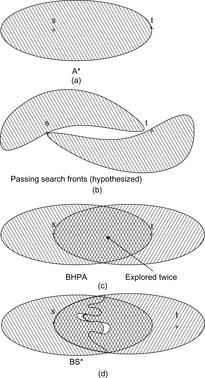 |
| Figure 9.25 |
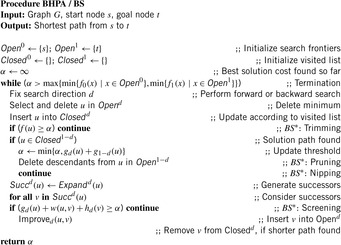
Although algorithm BS* saves a lot of time and memory, compared to BHPA, in experiments it still couldn't significantly outperform A* search. Usually the frontiers meet, and the optimal solution path is found early in the computation; most of the effort is in proving that this found path is indeed optimal.
9.6.2. *Bidirectional Front-to-Front Search
Over a long time, researchers believed that the experimental inefficiency of BHPA was due to the fact the search frontiers passed each other. Therefore, wave-shaping techniques were invented that would guide the two search frontiers toward each other. These algorithms use front-to-front evaluations that directly estimate the distance between the search frontiers.
The bidirectional heuristic front-to-front algorithm (BHFFA) computes the value f(u, v) = g0(u) + h(u, v) + g1(v) for all pairs (u, v) ∈ Open0 × Open1. Then it selects two nodes umin and vmin for expansion in the two search frontiers that minimize the f-value, f(umin, vmin) = min{f(u, v) | (u, v) ∈ Open0 × Open1}. Different than in front-to-end evaluation, the algorithm can admissibly terminate with the first solution path found. There are subtle problems with the front-to-front approach; the first version of BHFFA was wrong in the sense that it failed to find optimal solutions.
BHFFA was experimentally shown to improve on unidirectional search in terms of node expansions. However, the computational complexity is extremely high, and outweighs this advantage by far. In a straightforward implementation, each step requires n0 ⋅ n1 heuristic evaluations, where ni is the number of nodes in search frontier i. The total time complexity is O(n3), since there are at most n iterations for a total number of n expansions. When storing the result in O(n0 ⋅ n1) memory, the number of evaluations per expansion can be reduced to the number of successors of the expanded node, times the size of the opposite search frontier.
To ease this overhead, Politowski and Pohl proposed another important derivate of BHFFA, called d-node retargeting. It guides the search frontier only toward one “central” node in the opposite search frontier, the d-node, where d is fixed as the furthest search node from the origin. Every k iterations, the search direction is switched, and a new d-node is computed on the opposite search frontier.
Unfortunately, d-node retargeting is also not admissible. Moreover, parameter k has to be chosen carefully. For a small parameter k we will get worse solutions when the two search frontiers meet; for a larger value of k, we imitate unidirectional search.
Problems with maintaining two concurrently growing search trees can be avoided. A combination of forward and backward search is to look at one search tree that consists of pairs of forward and backward states. In each node either the forward or the backward state is expanded.
The most challenging question, however, is why bidirectional heurstic search algorithms often perform rather poorly in practice, whereas in blind search the savings of bidirectional state space traversals are obvious. One of the answers is found when looking at the number of nodes that A* explores with respect to a given search depth. We choose a simple Fifteen-Puzzle problem example together with Manhattan distance heuristic and A*. Figure 9.26 shows the number of generated nodes with respect to a growing search depth. In difference to breadth-first search the number of expanded nodes drop significantly at both ends. The reason is that the heuristic estimate for the nodes closer to the goal is better. According to the IDA* search tree prediction, in depth i we expect about NiP(c − i) nodes for large f-cost threshold values c. If we assume P to be approximately normal distributed and Ni to be approximately equal to bi with brute-force branching factor b, we often observe that the reduction in P for smaller values of x is larger than the growth of Ni, so that NiP(c − i) decreases exponentially also at the end.
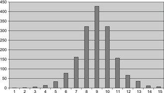 |
| Figure 9.26 |
The mean for the distribution is of course not exactly equal to half of the solution depth, but quite often it is not far off from this value. For our example with data values vi, i ∈ {1, …, 15} we compute  and
and  , so that we have a mean of 8.962.
9.6.3. Perimeter Search
Perimeter search tries to reap the benefits of front-to-front evaluations, while avoiding the computational efforts involved in retargeting the heuristics toward a continuously changing search frontier. The search direction only changes once. It conducts a depth-bounded breadth-first search starting from the goal node; the nodes on the final search frontier, called the perimeter, are stored. Then a forward search, starting from s, employs front-to-front evaluation with respect to these nodes. Algorithm PS* does this in a A*-like fashion, and algorithms IDPS* and BIDA* carry out IDA*. The difference between the latter two is that BIDA* removes nodes from the perimeter that cannot influence the heuristic evaluation. For retrieving the solution path, either the optimal solution path is stored with each node or all nodes together with pointers to their parents are stored as well. Moreover, whereas IDPS* evaluates the distance to each perimeter node, BIDA* is a little bit more elegant, since it introduced a condition to avoid the consideration of a number of perimeter nodes in the presence of consistent heuristic functions.
During the search we compute the heuristic value of each node outside the parameter as the minimal value of the heuristic estimate to each perimeter node, plus the diameter of the perimeter. The main advantages of perimeter search is that the minimum heuristic value together with the diameter is generally more accurate than a single heuristic, and the search can terminate once a state in the perimeter has been found. The disadvantages are that the memory requirements for storing the perimeter and, more crucially, that the multiple heuristic computations are considerable. For the former concern, it has been proven already that very small perimeters can significantly enhance the heuristic estimation. Later we will see that in the context of pattern databases the latter concern can be bypassed.
The forward search evaluation function is H(u) = minp∈P{h(u, p) + δ(p, t)}. This implies H(u) = δ(u, t) for all u ∈ P.
Theorem 9.1
(Admissibility of H) Heuristic H(u) is admissible if h is admissible.
Proof
We have to show that H(u) ≤ δ(u, t) for all u ∈ V P. Since h(u, v) ≤ δ(u, v) we have
Theorem 9.2
(Consistency of H) Heuristic H(u) is consistent if h is consistent.
Proof
We have to show that H(u) ≤ H(v) + w(u, v):
For the correctness of perimeter search, it is helpful to consider the perimeter reduction Gp of G, in which the entire perimeter is reduced to a single super node t* and all incoming edges to the perimeter starting at u are reassigned to w(u, t*) = w(u, v) + δ(v, t).
Theorem 9.3
(Perimeter Reduction) For all nongoal nodes u in the perimeter reduced graph GP of G, we have δG(s, t) = δGP(s, t*).
Proof
Let p = (u0, …, uk) be a solution path from s to t in G, then we have for a prefix p′ = (u0, …, ul) that (p′, t*) is a solution path in GP. We have g(p) = w(u0, u1) + ⋯ + w(ul − 1, ul) + w(ul, ul + 1) + ⋯ + w(uk − 1, uk). The condition w(ul, ul + 1) + ⋯ + w(uk − 1, uk) ≤ δ(ul, ut) implies that g(p) ≤ g(p′, t*). Moreover, for an optimal solution path we have δG(s, t) = δG(s, ul − 1) + w(ul − 1, ul) + δ(ul, t*) = δGP(s, t*).
*Improvements of Perimeter Search
The following update procedure has been suggested to save time in computing minp ∈ P{h(u, p) + δ(p, t)}. However, it requires O(|P|) storage at each node to store the estimated distance to the target through each perimeter node; therefore, for large problems it can be used only in conjunction with the iterative-deepening procedure (IDPS*).
The improvement is based on the observation that with a consistent heuristic, it holds for each v and u that |h(v) − h(u)| ≤ w(u, v), where w(u, v) is the weight of the edge between u and v. Thus, the estimate from v to a perimeter node can at most change by w(u, v), where u is the parent of v. Therefore, the heuristic value does not need to be recomputed if its value cannot change enough to affect the minimum.
The heuristic is used once fully for the start node at the beginning of the search for each perimeter node, and these estimates are stored, along with the index of the minimum. Next, when a node v is generated from u, the heuristic value of the current minimum is recomputed. The edge weight w(u, v) is then subtracted from the rest of the stored heuristic values; if any of these falls below the current minimum, it is recomputed using h, too.
In the Fifteen-Puzzle domain, BIDA* expands only a fraction of the nodes A* expands. This reduction has to be balanced with the increased computation time needed for the heuristic evaluation. It turns out that when varying the perimeter diameter, the overall running time exhibits a minimum at depth 16; at this point, it amounts to 27.4% of A*'s running time and 0.9% of its expansions.
When analyzing the improvements, it becomes clear that the benefit of the bidirectional approach lies primarily in a dynamically improved heuristic estimate. For example, in the Fifteen-Puzzle, using a perimeter of only 1 (which contains two nodes) saves already about half of the node generations of IDA*. The perimeter search discovers an improvement of the Manhattan distance heuristic under the name last move heuristic. In most cases the heuristic is increased by two units. The last move consists of bringing the blank into its goal position; therefore, before that, one of its neighbor tiles must be in the blank's goal position, which is not accommodated in the Manhattan distance.
Perhaps surprisingly, however, in other domains, it is hard to achieve any real improvements with perimeter search. This is, for example, the case in mazes under the same Manhattan distance. The reason is that the same perimeter achieves the same absolute improvement of the heuristic; however, since the solution length is longer by orders of magnitude, the relative impact is too insignificant. To obtain the same savings in expansions, a much larger perimeter would have to be computed, which would make perimeter search very expensive in terms of computation and memory.
*Front-to-Front Variants of Perimeter Search
To avoid the increased computational effort of front-to-front evaluations, it has been suggested to use the same scheme as in perimeter search, changing the direction only once and using the stored nodes of the first search in the second one, in conjunction with front-to-front evaluation. For the two search stages, different A*-like or IDA*-like algorithms can be instantiated (called BAA and BAI, respectively). If a Closed node of the backward stage is encountered, a solution path has been found, and it need not be expanded further (it can be nipped). The search terminates if the best solution found so far is no larger than the minimum f-value (in A*), respectively the next higher threshold (in IDA*).
In addition, bidirectional search allows for dynamic improvements of the heuristic, which are not possible in unidirectional search. One such method is called the Add-method. Let MinDiff be the minimum error of the heuristic on the perimeter around t, i.e.,  .
.
Lemma 9.1
(Nonincreasing Error of Heuristic) If h0 is consistent, then the error in the heuristic  cannot increase on an optimal solution path.
Proof
Let u and v be two successor nodes on an optimal path to t. Then
Using this lemma, the heuristic remains optimistic if we add the minimum error to it.
Theorem 9.4
(Quality Bound for Add-Method)  .
.
Proof
The optimal path from u to t must go through some perimeter node p:
Now unidirectional A* search wouldn't be affected at all by adding a constant to all heuristic values. However, recall that in BAI and BAA the current best solution is compared to the minimum estimate in Open; therefore, the addition can lead to earlier termination. For further optimization, to maximize MinDiff, the perimeter generation search can always select the node with the maximum error in the heuristic; this variant is called Add-BDA.
The second method, called the Max-method, uses the estimate h′0(u) = fmin, 1 − h1(u), where fmin, 1 is the minimum f-value of the perimeter,  .
.
Theorem 9.5
(Admissibility Max-Method)  .
.
Proof
The optimal path from u to t must go through some perimeter node p:
This dynamic evaluation is not necessarily always better than the static function, but since both are admissible, we can combine them as H0(u) = max{h0(u), fmin, 1 − h1(u)}.
In experimental studies, it was shown that Max-BAI with a transposition table can outperform IDA* (and all other bidirectional search algorithms) for the Fifteen-Puzzle, and that Add-BDA has outperformed A* (and all other bidirectional search algorithms) on maze problems.
*Near-Optimal Perimeter Search
Choosing f(u) = g(u) + λh(u) with λ > 1 in A* leads to inadmissible heuristics and nonoptimal solutions. Increasing values of λ results in finding solutions faster at the expense of an increased solution length. For perimeter search it seems irrational to calculate all these heuristics and then compute weighted versions. In near-optimal perimeter search the heuristic function is defined as h(u, t) and not as h(u, P), plus the depth of the perimeter as in perimeter search. For near-optimal perimeter search only constant time is needed to process each generated or expanded node. The match of a new node against the perimeter nodes that are saved in a hash table can be performed in a constant time.
Theorem 9.6
(Quality Bound on Perimeter Search) Let d be the depth of the perimeter P and let HP = minp ∈ P{h(p, t)} for an admissible heuristic h. Let δ(s, t) be the length of an optimal solution and W be the cost of the solution found by near-optimal perimeter search. Then we have
Proof
For the first inequality we note that the cost of any path that leads to the goal cannot be smaller than the optimal path cost. Since W is composed of the path cost g(u) and the heuristic estimate HP = minp ∈ P{h(p, t)} ≤ h(u) ≤ h*(u), the combined cost g(u) + HP cannot be larger than δ(s, t).
Since near-optimal perimeter search uses an admissible heuristic, 0 ≤ HP ≤ d and d − HP ≥ 0. Let u be the first encountered node on the perimeter; then we have W = g(u) + d. Since the cost function of A* and near-optimal perimeter search fulfill f(u) = g(u) + h(u) ≤ δ(s, t), we have g(u) + d ≤ δ(s, t) + d − h(u). In the worst case we can take the minimum heuristic value of all nodes in the perimeter and get W ≤ δ(s, t) + d − HP.
The value d − HP can be viewed as the maximum mistake of heuristic values among nodes in the perimeter.
9.6.4. Bidirectional Symbolic Breadth-First Search
As a by-product for symbolic search for the construction of symbolic pattern databases we have already seen the advantage of the transition relation Trans to perform backward search. Recall that for state sets Si we successively determine the preimages of the goal set, by computing for an increasing index i. Because the search is symbolic, large goal sets do not impose a burden to the search process.
In bidirectional breadth-first search, forward and backward search are carried out concurrently. On one hand, we have the symbolic forward search frontier ϕ{s}, and on the other, the backward search frontier ϕG. When the two search frontiers meet after f forward and b backward iterations we have found an optimal solution of length f + b. With the two horizons Open0 and Open1 the algorithm is implemented in pseudo code in Algorithm 9.16.
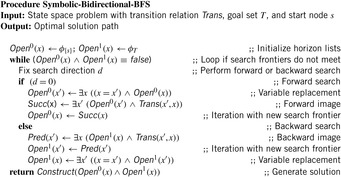
In a unit cost graph, the number of iterations remains equal to the optimal solution length f*. Solution reconstruction now proceeds from the established intersection to the respective starting states.
The selection of the direction of the search is often critical for a successful exploration. There are three simple criteria: BDD size, number of represented states, and smaller exploration time. Since the former two are not well suited to predict the computational efforts for the next iteration, the third criterion should be preferred.
9.6.5. *Island Search
Consider the road network of a city through which a river runs in a north-south direction (see Fig. 9.27). Suppose we are trying to find the shortest path from a western to an eastern destination; then the path is constrained to pass through one of the bridges over the river. The idea of island search is to improve search efficiency by breaking the path up into two components, before and after a bridge. Reaching a bridge can be regarded as a subgoal that has to be achieved first.
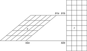 |
| Figure 9.27 |
In terms of a general search graph G = (V, E), we assume that we know of a (not too large) subset of nodes I ⊂ V, such that any solution path must contain one element; in other words, I represents a cut of G. This can allow us to improve search efficiency by means of a tighter heuristic estimate. Instead of using the goal distance h(u) from a node u to the goal t everywhere, we obtain a better bound for nodes before the cut as min{h(u|i)} for i ∈ I, where h(u|i) denotes the estimated length of a minimum path from u to t, constrained to pass through node i. For instance, in the route planning example, we can replace the air distance from the current location to the goal destination by sum of the air distance from the current location to the bridge, plus the air distance from the bridge to the target destination, minimized over all bridges.
Island search can be incorporated both into A*-like and IDA*-like search algorithms. In the original paper, the A*-algorithm is described using two Open and Closed lists; however, this is not strictly necessary. It is sufficient if each node stores an additional flag indicating whether its generating path contains an ancestor in I. When a node is expanded, the successors inherit its flag, unless the node is in I, in which case it is switched on. Depending on its value, the h-value is estimated either conventionally or using the constraint form.
Island search differs from A* or IDA* essentially only in the improved heuristics; therefore, if the latter one is admissible, the algorithm is guaranteed to find an optimal path, if one exists.
Moreover, suppose that the triangle equality h(x, y) ≤ h(x, z) + h(z, y) holds for the heuristic estimate; this is obviously true for the air distance metric in our example. Then, the A* variant of island search is at least as efficient as A*; that is, it expands no more nodes.
The original algorithm has been generalized to more than two islands. In this scenario, there is a user-supplied lower-bound E on the minimum number of bridges that have to be passed on an optimal solution path. Each node stores a set of flags for the cuts passed by its ancestors; the goal distance is used as the heuristic only if this set has E elements.
The practical results of island search depend on how well the search graph can be partitioned. In general, this must be done prior to the search in a domain-specific way. It is important to obtain a small cut size: This limits the increased computation cost of the heuristic, and usually leads to larger improvements. For example, in a route planning application we could partition the road map into zones of urban areas, which are connected to each other by relatively few highways and major roads.
9.6.6. *Multiple-Goal Heuristic Search
Most of the search algorithms we have considered in previous chapters work with multiple goal states for which the condition Goal is tested. However, for bidirectional search so far we are limited to one-to-one shortest path search. Moreover, perimeter search has extended the goal set from one to many states and we would like to avoid a one-to-many heuristic frontier calculation.
The three-peg Towers-of-Hanio problem illustrates the power of recursion. To move n disks from peg 1 to peg 2, first move (n − 1) disks from peg 1 to peg 3, then move disk n from peg 1 to peg 2, then move (n − 1) disks from peg 3 to peg 2. This leads to 2n − 1 moves. With three towers and n disks, the minimum number of moves is 2n − 1, so that the strategy is optimal.
An unproven conjecture on the four-peg Towers-of-Hanio problem (see Fig. 9.28) states that an optimal solution begins by forming a substack of the k-smallest disks, then moving the rest, and then moving those k again, with k to be determined. If in the four-peg n-disk Towers-of-Hanio problem we take two bits to encode the peg on which it is placed we arrive at a state vector of length 2n bits.
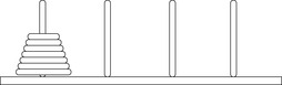
Based on the conjecture the minimum number of moves can be computed. The results are shown in Table 9.3. The numbers have been validated with parallel external heuristic search with up to 30 disks, which corresponds to a state space size of 430 states. The parallel search explored over 7.1 million states and required about 1.28 terabytes disk space.
For the Towers-of-Hanio problem the goal state and initial state are symmetrical. This allows the search depth in the four-peg problem to be cut to a half. The goal of the heuristic search was any middle state in which all but the largest disk are distributed over the two nongoal and noninitial pegs. If a middle state is found in depth l, then a complete solution in depth 2l + 1 can always be constructed. A depth 1,025 search for the 30-peg problem can thus be reduced to depth 512 to prove that no smaller solution exists.
The size of a single-goal pattern database is limited by the size of main memory, which by 1 GB is 230 bytes. If we assume that the abstract solution length is below 256 steps, a pattern database is bound to 15 disks. To construct the pattern database with 15 pegs all states in which the 15 disks are distributed among two pegs are generated and assigned to a depth zero for initializing the backward heuristic search. Then the entire state space size of 415 states is generated.
Multiple-goal pattern database search can overcome limitations of perimeter search. When constructing the database, we can seed backward database construction with all the states in the perimeter. During the overall search the minimum heuristic estimate is found by a simple table lookup. This technique requires that perimeter and abstract space computation are compatible.
9.7. Summary
Scaling a problem often implies that expanding a state involves new actions and increases the internal computation time for generating the heuristic and for the heuristic evaluation of the successors. In extreme cases, internal time exceeds hard disk access time. We have divided this chapter on distributed search into two equally important parts: one on parallel search and one on multidirectional search. If we have more processors at hand, then any multidirectional search can be parallelized, even if some techniques may impose much communication overhead.
Parallel search algorithms are designed to solve algorithmic problems using a network of processes while distributing the workload among them. Processes communicate via files or message passing. An efficient solution is obtained, if different tasks can be distributed in a way that working power is effectively used. A speedup is expected if the load is distributed uniformly with low interprocess communication. Internal workload is divided among different processors either residing on the same or on different machines.
Synchronicity refers to what happens when a process completes its task; either one process waits for the other to complete their tasks, or it starts working on a new task immediately. In synchronous parallel search each node of the search space is assigned to one process, which performs a search on it. Subsequent work is distributed by this process to idle recipient ones. In this manner eventually all processes receive work and perform sequential search. Workload is distributed via sharing the work that is present on local stacks. Enforcing a synchronous execution usually increases the communication complexity. In asynchronous parallel search workload will not be balanced among different processes. The only shared information that is broadcast are current upper bounds and solution qualities. As a side effect, a different timing for the information exchange can lead to a nondeterministic behavior. On the other hand, the nondeterminism does not necessarily induce that the computed result is incorrect. The established solution cost is either the value of the best solution found, or the value of the best solution to the remaining subproblems. In such an asynchronous setting not all processes have complete search knowledge, such that information exchange is delayed.
We looked at different parallel implementations for depth-first-inspired search strategies, including parallel branch-and-bound and parallel iterative-deepening A* search. For the elimination of duplicates a (static or dynamic) function distributing states to the processes is crucial, inducing lookup requests or entire states to be communicated. A loosely coupled (asynchronous) computation is often faster than a tight (synchronous) one, but requires structural knowledge of the problem. Here the search tree is often generated to some search depth, and the search frontier distributed among the different processors, since one option for load balancing large stacks is split. Among the options for IDA* with parallel window search a rather simple parallelization has been presented. For parallelizing A* search, the search frontier has to be maintained in appropriate data structures. For shared memory architectures treaps trade access priority with the best-first ordering of keys induced by the f-value. For more loosely coupled, so-called local A* search approaches, load balancing together with controlling the extra efforts for expanding suboptimal states becomes a challenge.
With external parallel breadth-first and best-first search we then suggested an improved distributed duplicate detection scheme for multiple processors and multiple hard disks. We assumed a typical network scenario, where computers are interconnected through Ethernet or over TCP/IP. The computers have access to a shared hard disk through a network file system and a local hard disk can be present at each computer. The setting extends to multicore or multiple-processor systems. External designs often lead to new solutions for parallel computing. Additional to parallelizing delayed duplicate detection, we also studied parallel structured duplicate detection. To exploit larger joint RAM capacities in a computer network pattern-oriented, memory-based heuristics are evaluated in parallel. As an example, a client-server architecture for solving the (n2 − 1)-Puzzle has been discussed under the assumption that computing the heuristic takes more time than generating the successor set. With the distribution of disjoint pattern databases each client is responsible for (all) the pattern database(s) that have a specific tile in their pattern. It exploits the fact that pattern databases are selected based on the tile that moves. Individual RAM requirements are reduced, allowing larger pattern databases to be kept on one process.
Table 9.4 summarizes the parallel search algorithms that have been introduced. We provide information on how the algorithm performs duplicate detection, if it is synchronous or asynchronous, whether the node set is kept local or global if the approach is incremental (improves solution quality over time), and if it reports the optimal solution at termination time.
We have seen significant search improvements by integrating GPU computation. Speedups of more than one order of magnitude on a single, moderately advanced graphics card are possible, especially on more recent or multiple cards. We restricted our exposition to large-scale breadth-first search. Many other external memory algorithms that have been discussed in this book are also streamed and are suggested to be ported to the GPU.
As bidirectional algorithms we have introduced BS/BHPA and BHFFS, which use either front-to-end or front-to-front evaluations. Solutions quality is usually gradually improved. We have illustrated why the prospects on savings driven from bidirectional breadth-first search have not been fulfilled in search practices. As one solution, perimeter search avoids merging two opposite-directed search heuristics and uses complete search at one end of the search space to increase the effectiveness for a search from the other side, since all nodes of the perimeter have to be stored. Island Search is a multidirectional algorithm that exploits the structure of problem space to partitioning it into different pieces that are searched individually.
Table 9.5 summarizes the bi- and multidirectional search algorithms. We denote the state representation, the applied search approach in forward and backward search (if any), whether the algorithms improve the solution quality over time (anytime), and if it is optimal at the end.
Bidirectional search can already accelerate single-processor search, namely when the processor time-slices between the two search directions. It is also possible to implement bidirectional search on more than two processors, for example, by using the search methods discussed in the chapter to distribute the workload of the search in one (or both) directions.
9.8. Exercises
9.1 Message passing interface libraries like MPI provide basic routines for message handling between different processes. Explain how critical sections of read and writes are to be avoided in MPI and compare the results with the alternative communication via (message) files as described in the text.
9.2 Bounded DFS depends on how information is exchanged. Produce pseudo code for two different information sharing approaches.
9.3 Consider the set of numbers (a1, …, a8) = (5, 3, 9, 4, 6, 2, 4, 1).
1. Explain the working of the parallel computation for computing the sum of a1 … a8 by displaying the array after each traversal of the loop of the procedure Sum.
2. Explain the working of the parallel computation for computing the prefix sum a1 … aj by displaying the array after each traversal of the loop of the procedure Prefix-Sum.
3. Show how procedure Prefix-Sum can be made work-optimal.
4. Search an implementation for the GPU (e.g., in CUDA) on the Internet and explain it.
9.4 To simulate a finite-state automaton using prefix sum computations use state set Q = {1, 2, 3, 4} and transition alphabet Σ = {a, b} as an example. Let q0 = 1 and let δ consist of the eight transitions  ,
,  and
and  as shown in Figure 9.29.
Let the input be string abbaabba.
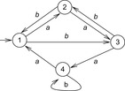
1. Compute the prefix sum over the associate function ⊗ that combines the sequential application of the transitions. For example, the combined transition function for string ab is 1 → 1, 2 → 2, 3 → 4, and 4 → 3, since 1 → 2 ⊗ 2 → 1 results in 1 → 1.
2. Denote the state that is reached for each possible prefix by inserting the initial state q0 in the transition function.
9.5 Use the solution of the previous exercise to compute the sum of two numbers x and y in binary in parallel logarithmic time.
1. Devise a two-state finite-state automata for propagating the carry bit. A state in this automata represents the carry bit from the i-th state to the (i + 1) th state. It depends on the sum of the two bits of xi and yi, so that the transition alphabet is Σ = {0, 1, 2}.
3. Compute the result of the addition. For each bit position the carry bit has to be added to the input bits. If the solution is even then the result is 0, otherwise 1.
9.6 Show how to use prefix sums to eliminate duplicates in a sorted sequence. Use an additional array to mark the elements that are the same.
9.7 Insert (17, 0) in the treap depicted in Figure 9.9.
1. Where is the node containing (17, 0) finally located?
2. How many rotation steps do you need to satisfy the treap property? Distinguish between left and right rotations.
3. Display the treap after each rotation step.
9.8 Consider a treap in the form of a randomized search tree for a set S of n numbers, where the priorities are uniformly distributed random numbers.
1. Show that the average path in a randomized search tree has the length O(lg n).
2. Compute the average case time for insertion. (This is a tough one, since you have to consider all permutations of the numbers {1, …, n}.)
3. Compute the average case time for deletion. Can you reuse the result of part (b)?
9.9 Sort large state sets (e.g., random strings) on the GPU.
• How can Bitonic Sort be of help?
• Can you beat CPU Quicksort?
• Discuss a strategy to parallelize Quicksort. What problems have to be resolved?
9.10 Transform the alignment of alternating black and white checkers depicted on the left side of Figure 9.30 into the arrangement shown on the right side of Figure 9.30. In this Checkers Rearrangement problem you are allowed to move only two checkers of different, colors at a time, preserving their original order and the alignment. You may introduce gaps as needed.
1. Find a solution to the problem by hand. Work backward to reduce the set of options.
2. Use an evaluation function for backward search that computes the number of color transitions to apply a greedy heuristic search reasoning.
9.11 Consider two jugs: one that contains seven units of water, and one that contains three units of water.
1. Find a solution sequence of fill and pouring operators that will result in one jar containing five units of water.
2. Work backward to obtain the solution more efficiently.
9.12 Draw a histogram on the number of expanded (or generated) nodes of A* in the Fifteen-Puzzle with Manhattan distance with respect to a growing search depth for the instance (14 1 9 6 4 8 12 5 7 2 3 0 10 11 13 15). Compare your result with respect to bidirectional breadth-first search.
9.13 Take the distributed search model by Vitter/Shriver for a problem graph G = (V, E) with locality L to be searched with N processors each having local disks. Show that parallel external BFS requires  I/Os.
I/Os.
9.14 Show that for consistent heuristics parallel external A* terminates with the shortest path from an initial state to a target state, and does not expand any node that has a higher f-value than a state in T.
9.15 This exercise addresses the diameter of Towers-of-Hanoi problem, namely the largest distance of any node from the initial state.
1. For the three-peg Towers-of-Hanoi problem show that the minimum number of 2n − 1 moves is the diameter of the problem by performing a complete BFS.
2. Show that for the four-peg Towers-of-Hanoi problem the depth is not always equal to the depth. While the condition is satisfied for smaller values n, for the 15-disk it is not. Run BFS on the 15-disk problem to validate that the optimal solution length is 129 and the diameter is 130. How many states are located in depth 130?
9.16 Compute all Fifteen-Puzzle instances that lie on a perimeter of size 3 around the goal node.
9.17 Implement IDA* with perimeter search to solve some random instances of the Fifteen-Puzzle problem.
9.18 Suppose the unit cost graph of Figure 9.27. Determine the intermediate f-values at b1b and b2b using
1. No additional heuristic.
2. A heuristic that counts the number of nonhorizontal lines between the actual node and the goal node (e.g., h(s) = 4).
Illustrate how Island Search continues given the information at the two nodes.
9.9. Bibliographic Notes
The textbook by Jájá (1992) covers the basic concepts of parallel computation. For the advanced readers the textbook by Zomaya (1996) may be appropriate. Applications of prefix sums have been studied by Eppstein and Galil (1988).
A number of parallel and distributed approaches to search have considerably improved the performance of the search process. Several parallelizations have been proposed for the branch-and-bound procedure with best-first traversal strategy.
Kumar, Ramesh, and Rao (1987) have given a survey on parallel best-first search. Kale and Saletore (1990) have considered parallel state space search for a first solution with consistent linear speedups. Minimal parallel window search is due to Powley and Korf (1991). Mahapatra and Dutt (1999) have analyzed parallel memory-restricted search and proposed an algorithm that iteratively extrapolates cost bounds. The application area is the traveling salesman problem. Exact extrapolations have been found via least-square curve fitting, and faster approximate extrapolations have been derived. A distributed termination criterion is due to Dijkstra and Scholten (1979).
The parallel search bench ZRAM, which solved the Fifteen-Puzzle by showing that the hardest initial configuration requires 80 moves to be solved, has been developed by Bruengger, Marzetta, Fukuda, and Nievergelt (1999). The authors discovered two previously unknown positions, requiring exactly 80 moves to be solved. Large-scale parallel breadth-first search with hash-based delayed duplicate elimination has been implemented by Korf and Schultze (2005) to completely enumerate all states in the Fifteen-Puzzle. Zhou and Hansen (2007b) have shown how to parallelize structured duplicate detection.
Different load balancing algorithms have been discussed by Dutt and Mahapatra (1994) while global and local hashing strategies for duplicate detections have been studied in Dutt and Mahapatra (1997). Adaptive parallel iterative-deepening A* by Cook and Varnell (1998) combines the benefits of many different approaches to parallel heuristic search. Results are generated from Fifteen-Puzzle problems, robot arm motion problems, artificial search spaces, and planning problems, and indicate that the system is able to greatly reduce the search time for these applications. General and parallel branch-and-bound search has been discussed by Nau, Kumar, and Kanal (1984). A parallel implementation PRA* for the connection machine has been provided by Evett, Hendler, Mahanti, and Nau (1990). Transposition-driven scheduling has been introduced by Romein, Plaat, Bal, and Schaeffer (1999) and extended to two-player games by Kishimoto (1999). Recent implementation of A* and its derivatives on multicore machines include HDA* by Kishimoto, Fukunaga, and Botea (2009) and PBFS by Burns et al. 2009a and Burns et al. 2009b. The former improves on transposition-driven scheduling and the latter improves on structured duplicate detection. Another refinement including edge partitioning suited to multicore search has been presented by Zhou, Schmidt, Hansen, Do, and Uckun (2010).
Lock-free (or wait-free) hash tables have been shown to be effective in state space search for reachability purposes by Laarman, van de Pol, and Weber (2010). The locking is realized without explicit lock variables using the atomic compare-and-swap operation. Sulewski, Edelkamp, and Kissmann (2011) have shown a domain-independent planner that exploits processing power available on the graphics card. To enhance precondition checks as well as assignments to effect variables on the GPU, a postfix notation of the expressions is used, and for duplicate detection, lock-free hash tables that yield optimal solutions are employed.
In the area of formal methods various authors have proposed ways of solving the problem of distributing the memory requirements over a cluster of workstations. Perhaps one of the first efforts is by Aggarwal, Alonso, and Courcoubetis (1988). Stern and Dill (1997) have employed a hash-based partitioning scheme to divide the whole state space into multiple computing nodes. The proposed approach was implemented on top of the Murϕ verifier. Lerda and Sisto (1999) have experimented with a different partition function. The rationale behind their hash function is that a transition usually performs only few local changes in a system, so that with a high probability a successor might belong to the current node. Haverkort, Bell, and Bohnenkamp (1999) have introduced distributed search for stochastic Petri nets. Distributed verification in μ calculus has been reported by Bollig, Leucker, and Weber (2001) and for CTL* by Inggs and Barringer (2006). There are attempts by Behrmann, Hune, and Vaandrager (2000) to consider real-time settings and by Garavel, Mateescu, and Smarandache (2001) and Bollig et al. (2001) for SAT solving in a distributed environment. Edelkamp, Jabbar, and Sulewski (2008a) have parallized a C++ software model checker using state reconstruction and incremental hashing techniques. Distribution based on partitioning the Büchi automata has been contributed by Lluch-Lafuente (2003a). Another approach for distributed model checking based on BDDs has been reported by Grumberg, Heyman, and Schuster (2006).
Parallel external search with delayed duplication has been introduced by Jabbar and Edelkamp (2006) for model checking safety properties in SPIN. It shows that the approach is compatible with state vectors of varying length. The approach has been extended to LTL properties by Edelkamp and Jabbar (2006c). A wide body of important results on distributed verification for both safety and liveness is contributed by the Paradise Lab mostly implemented in the Divine environment Barnat et al. (2006). A distributed cycle detection algorithm for LTL model checking based on parallel breadth-first search has been reported by Barnat, Brim, and Chaloupka (2003). An extension contributes an external memory variant of the same algorithm (Barnat, Brim, and Simecek, 2007). With depth-slicing Holzmann and Bosnacki (2007) have presented a method for N-core safety model checking. Their algorithm for liveness properties is limited to dual-core systems.
Owens et al. (2008) surveys the remarkable increase in the performance and capabilities of GPUs. They have outpaced CPUs in numerical algorithms as shown by Krueger and Westermann (2003) and by Harris, Sengupta, and Owens (2007). Applications include studying the folding behavior of proteins by Jaychandran, Vishal, and Pande (2006) and the simulation of biomolecular systems by Phillips et al. (2005). Since the memory transfer between the card and main board on the express bus is about one gigabyte per second, GPUs have become an apparent candidate to speed up large-scale computations like sorting numerical data on disk, as shown by Govindaraju, Gray, Kumar, and Manocha (2006) and by Cederman and Tsigas (2008). Its application for sorting-based delayed duplicate detection is apparent. By using perfect hash functions there is work by Edelkamp, Sulewski, and Yücel (2010b) on exploring single-agent search problems on the GPU and by Edelkamp, Sulewski, and Yücel (2010a) on solving two-player games. Explicit-state and probabilistic model checking problems have been ported to the GPU by Bosnacki, Edelkamp, and Sulewski (2009) and by Edelkamp and Sulewski (2010).
Priority search trees have been invented by McCreight (1985). The treap data structure has been proposed by Aragon and Seidel (1989) and the A* implementation based on them has been implemented by Cung and LeCun (1994).
One of the first references to bidirectional search is Pohl (1971). The effectiveness of method was surveyed later by Kaindl and Kainz (1997). The algorithm BIDA* was introduced by Manzini (1995). BHPA was invented by Pohl (1969). Kwa (1994) suggested BS* as an improvement to BHPA. The front-to-front strategy has been proposed by DeChampeaux and Sint (1977). The first version of BHFFA was not able to grant optimality, a problem that was resolved by DeChampeaux in 1983. Politowski and Pohl (1984) suggested the use of d-nodes to focus the search. A time improvement has been contributed by Eckerle and Ottmann (1994). By the virtue of states pairs, of which either the first or the second state is expanded, there is an interesting transformation of bidirectional search to unidirectional frontier search (Felner, Moldenhauer, Sturtevant, and Schaeffer, 2010).
Perimeter search has been introduced by Dillenburg and Nelson (1994) and independently by Manzini (1995). A good exposition can be found in the PhD thesis of Dillenburg (1993). Improvements to perimeter search and near-optimal perimeter search are provided in the PhD thesis of Felner (2001). The proof that very small perimeters can significantly enhance the heuristic estimation is given in Linares Lòpez and Junghanns (2003).
Two approaches combine pattern database construction with perimeter search. Anderson, Schaeffer, and Holte (2007) have proposed partial pattern databases that consist of a set of abstract nodes and their distance to the goals less than some lower-bound threshold value. Felner and Ofek (2007) have used a perimeter to seed the pattern database, such that the perimeter acts as a goal node. Multiple-goal heuristic search for solving the four-peg Towers-of-Hanoi problem has been implemented by Korf and Felner (2007), a work that also suggests the use of perimeter pattern databases. Another multiple-goal task for focused web crawling has been addressed by Chakrabarti, van den Berg, and Dom (1999) and by Diligenty, Coetzee, Lawrence, Giles, and Gori (2000).
..................Content has been hidden....................
You can't read the all page of ebook, please click here login for view all page.