
Chapter 18. Computational Biology
This chapter gives a general introduction to biological pathway and multiple sequence alignment problems. For the latter, a sparse-memory search approach is presented.
Keywords: computational biology, biological network, biological metabolic pathway, biological signal transduction pathway, multiple sequence alignment, Hirschberg's algorithm, iterative-deepening dynamic programming, sparse representation of solution paths, pairwise alignment, improved heuristic
Computational biology or bioinformatics is a large research field on its own. It is dedicated to the discovery and implementation of algorithms that facilitate the understanding of biological processes. The field encompasses different areas, such as building evolutionary trees and operating on molecular sequence data. Many approaches in computational biology refer to statistical and machine learning techniques. We concentrate on aspects for which the paradigm of state space search applies.
First of all, we observe a tight analogy between biological and computational processes. For example, generating test sequences for a computational system relates to generating experiments for a biological system. On the other hand, many biochemical phenomena reduce to the interaction between defined sequences.
We selected two problems as representatives for the field and in which heuristics have been applied for increasing the efficiency of the exploration. On one hand, we analyze Biological Pathway problems, which have been intensively studied in the field of molecular biology for a long time. We show how these problems can be casted as state space search problems and we illustrate how one problem can be implemented as a planning domain to participate from the general planning heuristics.
On the other hand, we consider what has been denoted as the holy grail in DNA and protein analyses. Throughout the book, we have already made several references to Multiple Sequence Alignment. The core of this chapter aims at providing a coherent perspective and points out recent trends in research of this ubiquitous problem in computational biology.
18.1. Biological Pathway
The understanding of biological networks, such as (metabolic and signal transduction) pathways, is crucial for understanding molecular and cellular processes in the organism or system under study. One natural way to study biological networks is to compare known with newly discovered networks and look for similarities between them.
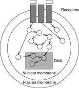
A Biological Pathway is a sequence of chemical reactions in a biological organism. Such pathways specify mechanisms that explain how cells carry out their major functions by means of molecules and reactions that produce regular changes. Many diseases can be explained by defects in pathways, and new treatments often involve finding drugs that correct those defects. An example of signaling pathways in a cell is illustrated in Figure 18.1.
We can model parts of the functioning of a pathway as a search problem by simply representing chemical reactions as actions. One example of the Biological Pathway domain is the pathway of the mammalian cell cycle control. There are different kinds of basic actions corresponding to the different kinds of reactions that appear in the pathway.
A simple qualitative encoding of the reactions of the pathway has five different actions: an action for choosing the initial substrates, an action for increasing the quantity of a chosen substrate (in the propositional version, quantity coincides with presence, and it is modeled through a predicate indicating if a substrate is available or not), an action modeling biochemical association reactions, an action modeling biochemical association reactions requiring catalysts, and an action modeling biochemical synthesis reactions. An encoding as a planning domain is provided in Figure 18.2.

The goals refer to substances that must be synthesized by the pathway, and are disjunctive with two disjuncts each. Furthermore, there is a limit on the number of input substrates that can be used in the pathway.
In extended versions both the products that must be synthesized by the pathway and the number of the input substrates that are used by the network are turned into preferences. The challenge here is finding paths that achieve a good trade-off between the different kinds of preferences.
Reactions have different durations and can happen if their input substrates reach some concentration level. Moreover, reactions generate their products in specific quantities. The refined goals are summations of substance concentrations that must be generated by the pathway.
18.2. Multiple Sequence Alignment
Despite their limitation to the moderate number of sequences, the research on exact algorithms for the Multiple Sequence Alignment problem is still going on, trying to push the practical boundaries further. They still form the building block of heuristic techniques, and incorporating them into existing tools could improve them. For example, an algorithm iteratively aligning two groups of sequences at a time could do this with three or more, to better avoid local minima. Moreover, it is theoretically important to have the “gold standard” available for evaluation and comparison, even if not for all problems.
Since MSA can be cast as a minimum-cost path finding problem, it is amenable to heuristic search algorithms developed in the AI community; these are actually among the currently best approaches. Therefore, though many researchers in this area have often used puzzles and games in the past to study heuristic search algorithms, recently there has been a rising interest in MSA as a test bed with practical relevance.
A number of exact algorithms have been developed that compute alignments for a moderate number of sequences. Some of them are constrained by available memory, some by the required computation time, and some by both. It is helpful to roughly group the approaches into two categories: those based on the dynamic programming paradigm, which proceed primarily in breadth-first fashion; and best-first search, utilizing lower and/or upper bounds to prune the search space. Some recent research, including the one introduced in Section 18.2.2, attempts to beneficially combine these two approaches.
The earliest Multiple Sequence Alignment algorithms were based on dynamic programming (see Sec. 2.1.7). We have seen how Hirschberg's algorithm (see Sec. 6.3.2) is able to reduce the space complexity by one dimension from O(Nk) to O(kNk−1), for k sequences of length at most N, by deleting each row as soon as the next one is completed; only a few relay nodes are maintained. To finally recover the solution path, a divide-and-conquer strategy recomputes the (much easier) partial problems between the relays.
Section 6.3.1 described how dynamic programming can be cast in terms of Dijkstra's algorithm, to do essentially the same, but relieving us from the necessity of explicitly allocating a matrix of size N3; this renders dynamic programming quickly infeasible when more than two sequences are involved. Reference counting has been introduced for Closed list reduction, already having a big practical impact on the feasibility of instances.
For integer edge costs, the priority queue (also referred to as the heap) can be implemented as a bucket array pointing to doubly linked lists, so that all operations can be performed in constant time. To expand a vertex, at most 2k−1 successor vertices have to be generated, since we have the choice of introducing a gap in each sequence. Thus, like dynamic programming, Dijkstra's algorithm can solve the Multiple Sequence Alignment problem in O(2kNk) time and O(Nk) space for k sequences of length ≤ N.
On the other hand, although dynamic programming and Dijkstra's algorithm can be viewed as variants of breadth-first search, we achieve best-first search if we expand nodes v in the order of an estimate (lower bound) of the total cost of a path from s to the t passing through v. Rather than the g-value as in Dijkstra's algorithm, we use  as the heap key, where h(v) is a lower bound on the cost of an optimal path from v to t; most of the time, the sum of optimal pairwise alignments is used.
Unfortunately, the standard linear-memory alternative to A*, IDA*, is not applicable in this case: Although it works best in tree-structured spaces, lattice-structured graphs like in the Multiple Sequence Alignment problem induce a huge overhead in duplicate expansions due to the huge number of paths between any two given nodes.
It should be mentioned that the definition of the Multiple Sequence Alignment problem as given earlier is not the only one; it competes with other attempts at formalizing biological meaning, which is often imprecise or depends on the type of question the biologist investigator is pursuing. In the following, we are only concerned with global alignment methods, which find an alignment of entire sequences. Local methods, in contrast, are geared toward finding maximally similar partial sequences, possibly ignoring the remainder.
18.2.1. Bounds
Let us now have a closer look on how lower and upper bounds are derived.
Obtaining an inaccurate upper bound on δ(s, t) is fairly easy, since we can use the cost of any valid path through the lattice. Better estimates are available from heuristic linear-time alignment programs.
In Section 1.7.6, we have already seen how lower bounds on the k-alignment are often based on optimal pairwise alignments; usually, prior to the main search, these subproblems are solved in a backward direction, by ordinary dynamic programming, and the resulting distance matrix is stored for later access.
Let U* be an upper bound on the cost of an optimal multiple sequence alignment G. The sum of all optimal alignment costs  for pairwise subproblems
  , call it L, is a lower bound on G. Carrillo and Lipman pointed out that by the additivity of the sum-of-pairs cost function, any pairwise alignment induced by the optimal multiple sequence alignment can at most be δ = U − L larger than the respective optimal pairwise alignment. This bound can be used to restrict the number of values that have to be computed in the preprocessing stage and have to be stored for the calculation of the heuristic: For the pair of sequences i, j, only those nodes v are feasible such that a path from the start node si, j to the goal node ti, j exists with total cost no more than Li, j+δ. To optimize the storage requirements, we can combine the results of two searches. First, a forward pass determines for each relevant node v the minimum distance d(si, j, v) from the start node. The subsequent backward pass uses this distance like an exact heuristic and stores the distance d(v, ti, j) from the target node only for those nodes with
  .
.
Still, for larger alignment problems the required storage size can be extensive. In some solvers, the user is allowed to adjust δ individually for each pair of sequences. This makes it possible to generate at least heuristic alignments if time or memory doesn't allow for the complete solution; moreover, it can be recorded during the search if the δ-bound was actually reached. In the negative case, optimality of the found solution is still guaranteed; otherwise, the user can try to run the program again with slightly increased bounds.
The general idea of precomputing simplified problems and storing the solutions for use as a heuristic is the same as in searching with pattern databases. However, these approaches usually assume that the computational cost can be amortized over many search instances to the same target. In contrast, many heuristics are instance-specific, such that we have to strike a balance.
18.2.2. Iterative-Deepening Dynamic Programming
As we have seen, a fixed search order as in dynamic programming can have several advantages over pure best-first selection.
• Since Closed nodes can never be reached more than once during the search, it is safe to delete useless ones (those that are not part of any shortest path to the current Open nodes) and to apply path compression schemes, such as the Hirschberg algorithm. No sophisticated schemes for avoiding back leaks are required, such as core set maintenance and dummy node insertion into Open.
• Besides the size of the Closed list, the memory requirement of the Open list is determined by the maximum number of nodes that are open simultaneously at any time while the algorithm is running. When the f-value is used as the key for the priority queue, the Open list usually contains all nodes with f-values in some range  ; this set of nodes is generally spread across the search space, since g(and accordingly h = (f − g)) can vary arbitrarily between 0 and fmin+δ. As opposed to that, if dynamic programming proceeds along levels of antidiagonals or rows, at any iteration at most k levels have to be maintained at the same time, and hence the size of the Open list can be controlled more effectively.
• For practical purposes, the running time should not only be measured in terms of iterations, but we should also take into account the execution time needed for an expansion. By arranging the exploration order such that edges with the same head node (or more generally, those sharing a common coordinate prefix) are dealt with one after the other, much of the computation can be cached, and edge generation can be sped up significantly. We will come back to this point in Section 18.2.5.
The remaining issue of a static exploration scheme consists of adequately bounding the search space using the h-values. A* is known to be minimal in terms of the number of node expansions. If we knew the cost δ(s, t) of a cheapest solution path beforehand, we could simply proceed level by level of the grid, however, only immediately prune generated edges e whenever  . This would ensure that we only generate those edges that would have been generated by algorithm A* as well. An upper threshold would additionally help reduce the size of the Closed list, since a node can be pruned if all of its children lie beyond the threshold; additionally, if this node is the only child of its parent, this can give rise to a propagating chain of ancestor deletions.
We propose to apply a search scheme that carries out a series of searches with successively larger thresholds until a solution is found (or we run out of memory or patience). The use of such an upper bound parallels that in the IDA* algorithm.
18.2.3. Main Loop
The resulting algorithm, which we will refer to as iterative-deepening dynamic programming (IDDP), is sketched in Algorithm 18.1. The outer loop initializes the threshold with a lower bound (e.g., h(s)), and, unless a solution is found, increases it up to an upper bound. In the same manner as in the IDA* algorithm, to make sure that at least one additional edge is explored in each iteration, the threshold has to be increased correspondingly at least to the minimum cost of a fringe edge that exceeded the previous threshold. This fringe increment is maintained in the variable minNextThresh, initially estimated as the upper bound, and repeatedly decreased in the course of the following expansions.
In each step of the inner loop, we select and remove a node from the priority queue of which the level is minimal. As explained later in Section 18.2.5, it is favorable to break ties according to the lexicographic order of target nodes. Since the total number of possible levels is comparatively small and known in advance, the priority queue can be implemented using an array of linked lists; this provides constant time operations for insertion and deletion.
Edge Expansion
The expansion of an edge e is partial (see Alg. 18.2). A child edge might already exist from an earlier expansion of an edge with the same head vertex; we have to test if we can decrease the g-value. Otherwise, we generate a new edge if its f-value exceeds the search threshold of the current iteration and its memory is immediately reclaimed. In a practical implementation, we can prune unnecessary accesses to partial alignments inside the calculation of the heuristic as soon as the search threshold has already been reached.

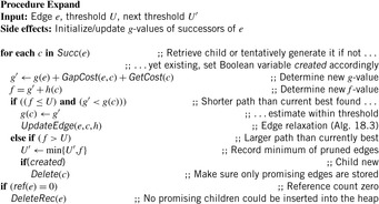
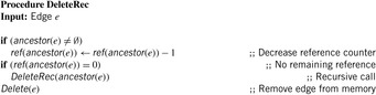
The relaxation of a successor edge within the threshold is performed by the subprocedure UpdateEdge (see Alg. 18.3). This is similar to the corresponding relaxation step in A*, updating the child's g- and f-values, its parent pointers, and inserting it into Open, if it is not already contained. However, in contrast to best-first search, it is inserted into the heap according to the antidiagonal level of its head vertex. Note that in the event that the former parent loses its last child, propagation of deletions (see Alg. 18.4) can ensure that only those Closed nodes continue to be stored that belong to some solution path. Edge deletions can also ensure deletion of dependent vertex and coordinate data structures (not shown in the pseudo code). The other situation that gives rise to deletions is if immediately after the expansion of a node no children are pointing back to it (the children might either be reachable more cheaply from different nodes, or their f-value might exceed the threshold).

The correctness of the algorithm can be shown analogously to the soundness proof of A*. If the threshold is smaller than δ(s, t), dynamic programming will terminate without encountering a solution; otherwise, only nodes are pruned that cannot be part of an optimal path. The invariant holds that there is always a node in each level that lies on an optimal path and is in the Open list. Therefore, if the algorithm terminates only when the heap runs empty, the best found solution stored will indeed be optimal.
The iterative-deepening strategy results in an overhead computation time due to reexpansions, and we are trying to restrict this overhead as much as possible. More precisely, we want to minimize the ratio  where nIDDP and nA* denote the number of expansions in IDDP and A*, respectively. We choose a threshold sequence U1, U2,… such that the number of expansions ni in stage i satisfies
  ; if we can at least double ni in each iteration, we will expand at most four times as many nodes as A*.
Procedure ComputeIncr stores the sequence of expansion numbers and thresholds from the previous search stages, and then uses curve fitting for extrapolation (in the first few iterations without sufficient data available, a very small default threshold is applied). We found that the distribution of nodes n(U) with an f-value smaller or equal to threshold U can be modeled very accurately according to the exponential approach  Consequently, to attempt to double the number of expansions, we choose the next threshold according to
18.2.4. Sparse Representation of Solution Paths
When the search progresses along antidiagonals, we do not have to fear back leaks, and are free to prune Closed nodes. We only want to delete them lazily and incrementally when being forced to by the algorithm approaching the computer's memory limit, however.
When deleting an edge e, the backtrack pointers of its child edges that refer to it are redirected to the respective predecessor of e, the reference count of which is increased accordingly. In the resulting sparse solution path representation, backtrack pointers can point to any optimal ancestors.
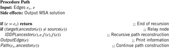
After termination of the main search, we trace back the pointers starting with the goal edge; this is outlined Alg. 18.5, which prints out the solution path in reverse order. Whenever an edge e points back to an ancestor e′ that is not its direct parent, we apply an auxiliary search from start edge e′ to goal edge e to reconstruct the missing links of the optimal solution path. The search threshold can now be fixed at the known solution cost; moreover, the auxiliary search can prune those edges that cannot be ancestors of e because they have some coordinate greater than the corresponding coordinate in e. Since also the shortest distance between e and e′ is known, we can stop at the first path that is found at this cost. To improve the efficiency of the auxiliary search even further, the heuristic could be recomputed to suit the new target. Therefore, the cost of restoring the solution path is usually marginal compared to that of the main search.
Which edges are we going to prune, in which order? For simplicity, assume for the moment that the Closed list consists of a single solution path. According to the Hirschberg approach, we would keep only one edge, preferably lying near the center of the search space (e.g., on the longest antidiagonal), to minimize the complexity of the two auxiliary searches. With additional available space allowing us to store three relay edges, we would divide the search space into four subspaces of about equal size (e.g., additionally storing the antidiagonals halfway between the middle antidiagonal and the start node respectively the target node). By extension, to incrementally save space under diminishing resources we would first keep only every other level, then every fourth, and so on, until only the start edge, the target edge, and one edge halfway on the path would be left.
Since in general the Closed list contains multiple solution paths (more precisely, a tree of solution paths), we would like to have about the same density of relay edges on each of them. For the case of k sequences, an edge reaching level l with its head node can originate with its tail node from level l − 1,…, l − k. Thus, not every solution path passes through each level, and deleting every other level could result in leaving one path completely intact, while extinguishing another totally. Thus, it is better to consider contiguous bands of k levels each, instead of individual levels. Bands of this size cannot be skipped by any path. The total number of antidiagonals in an alignment problem of k sequences of length N is k⋅N − 1; thus, we can decrease the density in  steps.
A technical implementation issue concerns the ability to enumerate all edges that reference some given prunable edge, without explicitly storing them in a list. However, the reference counting method described earlier ensures that any Closed edge can be reached by following a path bottom-up from some edge in Open. The procedure is sketched in Algorithm 18.6. The variable sparse denotes the interval between level bands that are to be maintained in memory. In the inner loop, all paths to Open nodes are traversed in a backward direction; for each edge e′ that falls into a prunable band, the pointer of the successor e on the path is redirected to its respective backtrack pointer. If e was the last edge referencing e′, the latter one is deleted, and the path traversal continues up to the start edge. When all Open nodes have been visited and the memory bound is still exceeded, the outer loop tries to double the number of prunable bands by increasing sparse.
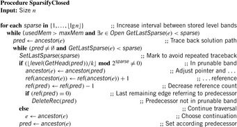
The procedure SparsifyClosed is called regularly during the search, for example, after each expansion. However, a naive version as described earlier would incur a huge overhead in computation time, particularly when the algorithm's memory consumption is close to the limit. Therefore, some optimizations are necessary. First, we avoid tracing back the same solution path at the same (or lower) sparse interval by recording for each edge the interval when it was traversed the last time (initially zero); only for an increased variable sparse can there be anything left for further pruning. In the worst case, each edge will be inspected  times. Second, it would be very inefficient to actually inspect each Open node in the inner loop, just to find that its solution path has been traversed previously, at the same or higher sparse value; however, with an appropriate bookkeeping strategy it is possible to reduce the time for this search overhead to O(k).
18.2.5. Use of Improved Heuristics
As we have seen, the estimator hpair, the sum of optimal pairwise goal distances, gives a lower bound on the actual path length. The tighter the estimator is, the smaller the search space the algorithm has to explore.
Beyond Pairwise Alignments
Kobayashi and Imai suggested applying more powerful heuristics by considering optimal solutions for subproblems of size m > 2. They proved that the following heuristics are admissible and more informed than the pairwise estimate.
• hall, m is the sum of all m-dimensional optimal costs, divided by  .
.
• hone, m splits the sequences into two sets of sizes m and k − m; the heuristic is the sum of the optimal cost of the first subset, plus that of the second one, plus the sum of all two-dimensional optimal costs of all pairs of sequences in different subsets. Usually, m is chosen close to k/2.
These improved heuristics can reduce the main search effort by orders of magnitudes. However, in contrast to pairwise subalignments, time and space resources devoted to compute and store higher-dimensional heuristics are in general no longer negligible compared to the main search. Kobayashi and Imai noticed that even for the case m = 3 of triples of sequences, it can be impractical to compute the entire subheuristic hall, m. As one reduction, they show that it suffices to restrict the search to nodes where the path cost does not exceed the optimal path cost of the subproblem by more than
This threshold can be seen as a generalization of the Carrillo-Lipman bound. However, it can still incur excessive overhead in space and computation time for the computation of the  lower-dimensional subproblems. A drawback is that it requires an upper bound, on which the accuracy of the algorithm's efficiency also hinges. We could improve this bound by applying more sophisticated heuristic methods, but it seems counterintuitive to spend more time doing so that we would rather use to calculate the exact solution. In spite of its advantages for the main search, the expensiveness of the heuristic calculation appears as a major obstacle.
An alternative is to partition the heuristic into (hyper-) cubes using a hierarchical oct-tree data structure; in contrast to “full” cells, “empty” cells only retain the values at their surface. When the main search tries to use one of them, its interior values are recomputed on demand. Still, this work assumes that each node in the entire heuristic is calculated at least once using dynamic programming.
One cause of the dilemma lies in the implicit assumption that a complete computation is necessary. The previous bound δ refers to the worst-case scenario, and can generally include many more nodes than actually required in the main search. However, since we are only dealing with the heuristic, we can actually afford to miss some values occasionally; although this might slow down the main search, it cannot compromise the optimality of the final solution. Therefore, we propose to generate the heuristics with a much smaller bound δ. Whenever the attempt to retrieve a value of the m-dimensional subheuristic fails during the main search, we simply revert to replacing it by the sum of the  -optimal pairwise goal distances it covers.
The IDDP algorithm lends itself well to make productive use of higher-dimensional heuristics. First and most important, the strategy of searching to adaptively increasing thresholds can be transferred to the δ-bound as well.
Second, as far as a practical implementation is concerned, it is important to take into account not only how a higher-dimensional heuristic affects the number of node expansions, but also their time complexity. This time is dominated by the number of accesses to subalignments. With k sequences, in the worst case an edge has 2k − 1 successors, leading to a total of  evaluations for
  . One possible improvement is to enumerate all edges emerging from a given vertex in lexicographic order, and to store partial sums of heuristics of prefix subsets of sequences for later reuse. In this way, if we allow for a cache of linear size, the number of accesses is reduced to
  correspondingly, for a quadratic cache we only need
  evaluations. For instance, in aligning 12 sequences using hall,3, a linear cache reduces the evaluations to about 37% within one expansion.
As mentioned earlier, in contrast to A*, IDDP gives us the freedom to choose any particular expansion order of the edges within a given level. Therefore, when we sort edges lexicographically according to the target nodes, much of the cached prefix information can be shared additionally across consecutively expanded edges. The higher the dimension of the subalignments, the larger the savings.
Trade-Off between Computation of Heuristic and Main Search
As we have seen, we can control the size of the precomputed subalignments by choosing the bound δ up to which f-values of edges are generated beyond the respective optimal solution cost. There is obviously a trade-off between the auxiliary and main searches. It is instructive to consider the heuristic miss ratio r, the fraction of calculations of the heuristic h during the main search when a requested entry in a partial Multiple Sequence Alignment has not been precomputed. The optimum for the main search is achieved if the heuristic has been computed for every requested edge (r = 0). Going beyond that point will generate an unnecessarily large heuristic containing many entries that will never be actually used. On the other hand, we are free to allocate less effort to the heuristic, resulting in r > 0 and consequently decreasing performance of the main search. Generally, the dependence has an S-shaped form.
Unfortunately, in general we do not know in advance the right amount of auxiliary search. As mentioned earlier, choosing δ according to the Carrillo-Lipman bound will ensure that every requested subalignment cost will have been precomputed; however, in general we will considerably overestimate the necessary size of the heuristic.
As a remedy, algorithm IDDP gives us the opportunity to recompute the heuristic in each threshold iteration in the main search. In this way, we can adaptively strike a balance between the two.
When the currently experienced fault rate r rises above some threshold, we can suspend the current search, recompute the pairwise alignments with an increased threshold δ, and resume the main search with the improved heuristics.
Like for the main search, we can accurately predict the auxiliary computation time and space at threshold δ using an exponential fitting. Due to the lower dimensionality, it will generally increase less steeply; however, the constant factor might be higher for the heuristic, due to the combinatorial number of  alignment problems to be solved.
A doubling scheme as explained previously can bound the overhead to within a constant factor of the effort in the last iteration. In this way, when also limiting the heuristic computation time by a fixed fraction of the main search, we can ensure as an expected upper bound that the overall execution time stays within a constant factor of the search time that would be required when using only the pairwise heuristic.
If we knew the exact relation between δ, r, and the speedup of the main search, an ideal strategy would double the heuristic whenever the expected computation time is smaller than the time saved in the main search. However, this dependence is more complex than simple exponential growth; it varies with the search depth and specifics of the problem. Either we would need a more elaborate model of the search space, or the algorithm would have to conduct explorative searches to estimate the relation.
18.3. Bibliographic Notes
Gusfield (1997) and Waterman (1995) have given comprehensive introductions to computational molecular biology. The definition of a pathway has been given by Thagard (2003). The mammalian cell cycle control has been described by Kohn (1999). It appeared as an application domain in the fifth international planning competition in 2006, where it was modeled by Dimopoulos, Gerevini, and Saetti. A recent search tool for the alignment of metabolic pathways has been presented by Pinter, Rokhlenko, Yeger-Lotem, and Ziv-Ukelson (2005). Given a query pathway and a collection of pathways, it finds and reports all approximate occurrences of the query in the collection.
Bosnacki (2004) has indicated a natural analogy between biochemical networks and (concurrent) systems with an unknown structure. Both are considered as a black box with unknown internal workings about which we want to check some property; that is, verify some hypothesis about their behavior. Test sequences can be casted as counterexamples obtained by search as observed by Engels, Feijs, and Mauw (1997). A suitable algorithm for inducing a model of a system has been developed by Angluin (1987). The algorithm requires an oracle that in this case is substituted by a conformance testing. Unlike model checking that is applied to the model of the system, (conformance) testing is performed on the system implementation. Also, conformance testing does not try to cover all execution sequences of the implementation. Rather than understanding the networks, the goal of Rao and Arkin (2001) is to design biological networks for a certain task.
FASTA and BLAST (see Altschul, Gish, Miller, Myers, and Lipman, 1990)), are standard methods for database searches. Davidson (2001) has employed a local beam search scheme. Gusfield (1993) has proposed an approximation called the star-alignment. Out of all the sequences to be aligned, one consensus sequence is chosen such that the sum of its pairwise alignment costs to the rest of the sequences is minimal. Using this “best” sequence as the center, the other ones are aligned using the “once a gap, always a gap” rule. Gusfield has shown that the cost of the optimal alignment is greater than or equal to the cost of this star alignment, divided by (2 − 2/k). The program MSA due to Gupta, Kececioglu, and Schaffer (1996) allows the user to adjust δ to values below the Carrillo-Lipman bound individually for each pair of sequences (Carrillo and Lipman, 1988).
For Multiple Sequence Alignment problems in higher dimensions, A* is clearly superior to dynamic programming. However, in contrast to the Hirschberg algorithm, it still has to store all the explored nodes in the Closed list to avoid “back leaks." As a remedy, Korf (1999) and Korf and Zhang (2000) have proposed to store a list of forbidden operators with each node, or to place the parents of a deleted node on Open with an f-value ∞. The approach by Zhou and Hansen (2004a) only requires the boundary to be stored.
The main algorithm IDDP as described in this chapter has been published by Schrödl (2005). The work by Korf, Zhang, Thayer, and Hohwald (2005) refers to a related incremental dynamic programming algorithm called iterative-deepening bounded dynamic programming.
McNaughton, Lu, Schaeffer, and Szafron (2002) have suggested an oct-tree data structure for storing the heuristic function. A different line of research tries to restrict the search space of the breadth-first approaches by incorporating bounds. Ukkonen (1985) has presented an algorithm for the pairwise alignment problem, which is particularly efficient for similar sequences; its computation time scales as O(dm), where d is the optimal solution cost.
Another approach for Multiple Sequence Alignment is to make use of the lower bounds h from A*. The key idea is the following: Since all nodes with an f-value lower than δ(s, t) have to be expanded anyway to guarantee optimality, we might as well explore them in any reasonable order, like that of Dijkstra's algorithm or dynamic programming, if we only knew the optimal cost. Even slightly higher upper bounds will still help pruning. Spouge (1989) has proposed to bound dynamic programming to nodes v where g(v)+h(v) is smaller than an upper bound for δ(s, t).
Linear bounded diagonal alignment (LBD-Align) by Davidson (2001) uses an upper bound to reduce the computation time and memory in solving a pairwise alignment problem by dynamic programming. The algorithm calculates the dynamic programming matrix one antidiagonal at a time, starting in the top-left corner, and working down toward the bottom-right corner. While A* would have to check the bound in every expansion, LBD-Align only checks the top and bottom cell of each diagonal. If, for example, the top cell of a diagonal has been pruned, all the remaining cells in that row can be pruned as well, since they are only reachable through it; this means that the pruning frontier on the next row can be shifted one down. Thus, the pruning overhead can be reduced from a quadratic to a linear amount in terms of the sequence length.
Progresses have been made to improve the scaling of the Multiple Sequence Alighnment algorithms. Niewiadomski, Amaral, and Holte (2006) have applied large-scale parallel frontier search with delayed duplicate detection to solve challenging (Balibase) instances, and Zhou and Hansen (2006a) have successfully improved the sparse-memory graph search with a breadth-first heuristic search.
..................Content has been hidden....................
You can't read the all page of ebook, please click here login for view all page.