Search in book...
Toggle Font Controls
Create new playlist

Name your new playlist

Playlist description (optional)
Sign In

Email address

Password

Forgot Password?

or

Continue with Facebook

Continue with Google
Sign Up

Full Name

Email address

Confirm Email Address

Password

or

Continue with Facebook

Continue with Google

Chapter 3. *Dictionary Data Structures

For the enhanced efficiency of A* this chapter discusses different dictionary data structures. Priority queues are provided for integer and total ordered keys. For duplicate elimination, hashing is studied, including provably constant access time. Moreover, maintaining partial states in form of substrings or subsets is considered.

Keywords: priority queue, 1-level bucket, 2-level bucket, Radix heap, van-Emde-Boas queue, heap, pairing heap, weak-heap, Fibonacci heap, relaxed weak queue, hash function, hash table, incremental hashing, universal hashing, perfect hashing, ranking and unranking, cuckoo hashing, suffix list, bitstate hashing, hash compaction, collapse compression, subset dictionary, unlimited branching tree, substring dictionary, suffix tree.

The exploration efficiency of algorithms like A* is often measured with respect to the number of expanded/generated problem graph nodes, but the actual runtimes depend crucially on how the Open and Closed lists are implemented. In this chapter we look closer at efficient data structures to represent these sets.

For the Open list, different options for implementing a priority queue data structure are considered. We distinguish between integer and general edge costs, and introduce bucket and advanced heap implementations.

For efficient duplicate detection and removal we also look at hash dictionaries. We devise a variety of hash functions that can be computed efficiently and that minimize the number of collisions by approximating uniformly distributed addresses, even if the set of chosen keys is not (which is almost always the case). Next we explore memory-saving dictionaries, the space requirements of which come close to the information-theoretic lower bound and provide a treatment of approximate dictionaries.

Subset dictionaries address the problem of finding partial state vectors in a set. Searching the set is referred to as the Subset Query or the Containment Query problem. The two problems are equivalent to the Partial Match retrieval problem for retrieving a partially specified input query word from a file of k-letter words with k being fixed. A simple example is the search for a word in a crossword puzzle. In a state space search, subset dictionaries are important to store partial state vectors like dead-end patterns in Sokoban that generalize pruning rules (see Ch. 10).

In state space search, string dictionaries are helpful to exclude a set of forbidden action sequences, like UD or RL in the (n² − 1)-Puzzle, from being generated. Such sets of excluded words are formed by concatenating move labels on paths that can be learned and generalized (see Ch. 10). Therefore, string dictionaries provide an option to detect and eliminate duplicates without hashing and can help to reduce the efforts for storing all visited states. Besides the efficient insertion (and deletion) of strings, the task to determine if a query string is the substring of a stored string is most important and has to be executed very efficiently. The main application for string dictionaries are web search engines. The most flexible data structure for efficiently solving this Dynamic Dictionary Matching problem is the Generalized Suffix Tree.

3.1. Priority Queues

When applying the A* algorithm to explore a problem graph, we rank all generated but not expanded nodes u in list Open by their priority

. As basic operations we need to find the element of the minimal f-value: to insert a node together with its f-value and to update the structure if a node becomes a better f-value due to a shorter path. An abstract data structure for the three operations Insert, DeleteMin, and DecreaseKey is a priority queue.

In Dijkstra's original implementation, the Open list is a plain array of nodes together with a bitvector indicating if elements are currently open or not. The minimum is found through a complete scan, yielding quadratic execution time in the number of nodes. More refined data structures have been developed since, which are suitable for different classes of weight functions. We will discuss integer and general weights; for integer cost we look at bucket structures and for general weights we consider refined heap implementations.

3.1.1. Bucket Data Structures

In many applications, edge weights can only be positive integers (sometimes for fractional values it is also possible and beneficial to achieve this by rescaling). As a general assumption we state that the difference between the largest key and the smallest key is less than or equal to a constant C.

Buckets

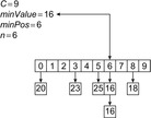
A simple implementation for the priority queues is a 1-Level Bucket. This priority queue implementation consists of an array of C + 1 buckets, each of which is the first link in a linked list of elements. With the array we associate the three numbers minValue, minPos, and n: minValue denotes the smallest f value in the queue, minPos fixes the index of the bucket with the smallest key, and n is the number of stored elements. The i th bucket

contains all elements v with

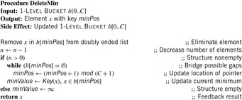
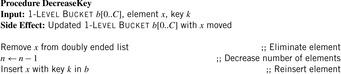
. Figure 3.1 illustrates an example for the set of keys {16, 16, 18, 20, 23, 25}. The implementations for the four main priority queue operations Initialize, Insert, DeleteMin, and DecreaseKey are shown in Algorithm 3.1, Algorithm 3.2, Algorithm 3.3 and Algorithm 3.4.

With doubly linked lists (each element has a predecessor and successor pointer) we achieve constant runtimes for the Insert and DecreaseKey operations, while the DeleteMin operation consumes O (C) time in the worst-case for searching a nonempty bucket. For DecreaseKey we generally assume that a pointer to the element to be deleted is available. Consequently, Dijkstra's algorithm and A* run in

time, where e is the number of edges (generated) and n is the number of nodes (expanded).

B9780123725127000031/f03-01-9780123725127.jpg is missing

Figure 3.1

Example for a 1-Level Bucket data structure.

Algorithm 3.1.

Initializing a 1-Level Bucket.

B9780123725127000031/u03-02-9780123725127.jpg is missing

Algorithm 3.2.

Inserting an element into a 1-Level Bucket.

B9780123725127000031/u03-03-9780123725127.jpg is missing

Algorithm 3.3.

Deleting the minimum element in a 1-Level Bucket.

Given that the f-value can often be bounded by a constant f_max in a practical state space search, authors usually omit the modulo operation mod (C + 1), which reduces the space for array b to O (C), and take a plain array addressed by f instead. If f_max is not known in advance a doubling strategy can be applied.

B9780123725127000031/u03-04-9780123725127.jpg is missing

Algorithm 3.4.

Updating the key in a 1-Level Bucket.

Multilayered Buckets

In state space search, we often have edge weights that are of moderate size, say realized by a 32-bit integer for which a bucket array b of size 2³² is too large, whereas 2¹⁶ can be afforded.

The space complexity and the worst-case time complexity O (C) for DeleteMin can be reduced to an amortized complexity of

operations by using a 2-Level Bucket data structure with one top and one bottom level, both of length

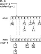
In this structure we have two pointers for the minimum position, minPosTop and minPosBottom, and a number nbot of bottom elements. Although each bucket in the bottom array holds a list of elements with the same key as before, the top layer points to lower-level arrays. If after a DeleteMin operation that yields a minimum key k no insertion is performed with a key less than k(as it is the case for a consistent heuristic in A*), it is sufficient to maintain only one bottom bucket (at minPosTop ), and collect elements in higher buckets in the top level; the lower-level buckets can be created only when the current bucket at minPosTop becomes empty and minPosTop moves on to a higher one. One advantage is that in the case of maximum distance between keys, DeleteMin has to inspect only the

buckets of the top level; moreover, it saves space if only a small fraction of the available range C is actually filled.

As an example, take C = 80, minPosTop = 2, minPosBottom = 1, and the set of element keys

. The intervals and elements in the top buckets are

, and

. Bucket b [2] is expanded with nonempty bottom buckets 1, 5, and 7 containing the elements 7, 11, and 13, respectively. Figure 3.2 illustrates the example.

B9780123725127000031/f03-02-9780123725127.jpg is missing

Figure 3.2

Example for 2-Level Bucket data structure.

Since DeleteMin reuses the bottom bucket in case it becomes empty, in some cases it is fast and in other cases it is slow. In our case of the 2-Level Bucket, let

be the number of elements in the top-level bucket, for the l th operation, then DeleteMin uses

time in the worst-case, where m_l is the number of elements that move from top to bottom. The term

is the worst-case distance passed by in the top bucket, and m_l are efforts for the reassignment, which costs are equivalent to the number of elements that move from top to bottom. Having to wait until all moved elements in the bottom layer are dealt with, the worst-case work is amortized over a longer time period. By amortization we have

operations. Both operations Insert and DecreaseKey run in real and amortized constant time.

Radix Heaps

For achieving an even better amortized runtime, namely

, a so-called Radix Heap maintains a list of

buckets of sizes 1, 1, 2, 4, 8, 16, and so on (see Fig. 3.3). The main difference to layered buckets is to use buckets of exponentially increasing sizes instead of a hierarchy. Therefore, only

buckets are needed.

For the implementation we maintain buckets

and bounds

with

and

. Furthermore, the bucket number

denotes the index of the actual bucket for key k. The invariants of the algorithms are (1) all keys in

are in

; (2)

; and (3) for all

we have

Figure 3.3

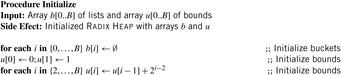
Example for a Radix Heap. The bottom row numbers denote current values of the bounds u and the top row numbers denote the size of the interval defined by two successive u-values.

The operations are as follows. Initialize generates an empty Radix Heap according to the invariants (2) and (3). The pseudo code is shown in Algorithm 3.5.

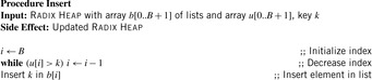
To insert an element with key k, in a linear scan a bucket i is searched, starting from the largest one (i = B). Then the new element with key k is inserted into the bucket

with

. The pseudo-code implementation is depicted in Algorithm 3.6.

B9780123725127000031/u03-05-9780123725127.jpg is missing

Algorithm 3.5.

Creating a Radix Heap.

B9780123725127000031/u03-06-9780123725127.jpg is missing

Algorithm 3.6.

Inserting an element into a Radix Heap.

B9780123725127000031/u03-07-9780123725127.jpg is missing

Algorithm 3.7.

Inserting an element into a Radix Heap.

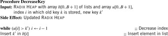
For DecreaseKey, bucket i for an element with key k is searched linearly. The difference is that the search starts from the actual bucket i for key k as stored in

. The implementation is shown in Algorithm 3.7.

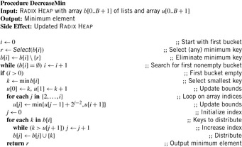
For DeleteMin we first search for the first nonempty bucket

and identify the element with minimum key k therein. If the smallest bucket contains an element it is returned. For the other case

is set to k and the bucket bounds are adjusted according to the invariances; that is,

is set to

and for

bound

is set to

. Lastly, the elements of

are distributed to buckets

and the minimum element is extracted from the nonempty smallest bucket. The implementation is shown in Algorithm 3.8.

B9780123725127000031/u03-08-9780123725127.jpg is missing

Algorithm 3.8.

Delete the minimum from a Radix Heap.

As a short example for DeleteMin consider the following configuration (written as

) of a Radix Heap

(see Fig. 3.4). Extracting key 0 from bucket 1 yields

. Now, key 6 and 7 are distributed. If

then the interval size is at most

. In

we have

buckets available. Since all keys in

are in

all elements fit into

Figure 3.4

Example for DeleteMin operation in a Radix Heap.

The amortized analysis of the costs of maintaining a Radix Heap uses the potential

for operation l. We have that Initialize runs in O (B), and Insert runs in O (B). DecreaseKey has an amortized time complexity in

, and DeleteMin runs in time

amortized. In total we have a running time of

for m Insert and l DecreaseKey and ExtractMin operations.

Utilizing this representation, A* runs in time

time. For current computers, the value of

for encompassing the entire integer range is small (32 or 64), so that A* on integers using a Radix Heap runs in linear time in practice.

Van Emde Boas Priority Queues

A Van Emde Boas Priority Queue is efficient when

for a universe

of keys. In this implementation, all priority queue operations reduce to successor computation, which takes

time. The space requirements are

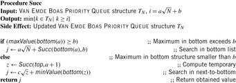
We start by considering a data structure T_N on the elements

defining only three operations: Insert (x), Delete (x), and Succ (x), where the two first ones have an obvious semantics and the last one returns the smallest item in T_N that is larger than or equal to x. All priority queue operations use the recursive operation Succ (x) that finds the smallest y in the structure T_N with

. For the priority queue data structure, DeleteMin is simply implemented as Delete (Succ (0)), assuming positive key values, and DecreaseKey is a combination of a Delete and an Insert operation.

Using an ordinary bitvector, Insert and Delete are constant-time operations, but Succ is inefficient. Using balanced trees, all operations run in time

. A better solution is to implement a recursive representation with

distinct versions of

. The latter trees are called bottom, and an element

is represented by the entry b in bottom (a). The conversion from i to a and b in bit-vector representation is simple, since a and b refer to the most and least significant half of the bits. Moreover, we have another version

called top that contains a only if a is nonempty.

Algorithm 3.9 depicts a pseudo-code implementation of Succ. The recursion for the runtime is

. If we set

then

so that

and

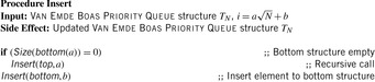
. The subsequent implementations for Insert and Delete are shown in Algorithm 3.10 and Algorithm 3.11. Inserting element x in T_N locates a possible place by first seeking the successor Succ (x) of x. This leads to a running time of

. Deletion used the doubly linked structure and the successor relation. It also runs in

time.

A Van Emde Boas Priority Queue k-structure is recursively defined. Consider the example k = 4 (implying N = 16) with the set of five elements

. Set top is a 2-structure on

based on the set of possible prefixes in the binary encoding of the values in S. Set bottom is a vector of 2-structures (based on the suffixes of the binary state encodings in S) with bottom

, bottom

, and bottom

, since

, and

. Representing top as a 2-structure implies k = 2 and N = 4, such that the representation of

with

, and

leads to a sub-top structure on

and two sub-bottom structures bottom

and bottom

B9780123725127000031/u03-09-9780123725127.jpg is missing

Algorithm 3.9.

Finding the successor in a Van Emde Boas Priority Queue.

B9780123725127000031/u03-10-9780123725127.jpg is missing

Algorithm 3.10.

Inserting an element in a Van Emde Boas Priority Queue.

B9780123725127000031/u03-11-9780123725127.jpg is missing

Algorithm 3.11.

Deleting an element from a Van Emde Boas Priority Queue.

To realize the structures in practice, a mixed representation of the element set is appropriate. On one hand, a doubly connected linked list contains the elements sorted according to the values they have in the universe. On the other hand, a bitvector b is devised, with bit i denoting if an element with value b_i is contained in the list. The two structures are connected via links that point from each nonzero element to an item in the doubly connected list. The mixed representation (bitvector and doubly ended leaf list) for the earlier 4-structure (without unrolling the references to the single top and four bottom structures) is shown Figure 3.5.

B9780123725127000031/f03-05-9780123725127.jpg is missing

Figure 3.5

An example of a 4-structure for the Van Emde Boas Priority Queue.

3.1.2. Heap Data Structures

Let us now assume that we can have arbitrary (e.g., floating-point) keys. Each operation in a priority queue then divides into compare-exchange steps. For this case, the most common implementation of a priority queue (besides a plain list) is a Binary Search Tree or a Heap.

Binary Search Trees

A Binary Search Tree is a binary tree implementation of a priority queue in which each internal node x stores an element. The keys in the left subtree of x are smaller than (or equal) to the one of x, and keys in the right subtree of x are larger than the one of x. Operations on a binary search tree take time proportional to the height of the tree. If the tree is a linear chain of nodes, linear comparisons might be induced in the worst-case. If the tree is balanced, a logarithmic number of operations for insertion and deletion suffice. Because balancing can be involved, in the following we discuss more flexible and faster data structures for implementing a priority queue.

Heaps

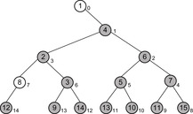
A Heap is a complete binary tree; that is, all levels are completely filled except possibly the lowest one, which is filled from the left. This means that the depth of the tree (and every path length from the root to a leaf) is

. Each internal node v satisfies the heap property: The key of v is smaller than or equal to the key of either of its two children.

Complete binary trees can be embedded in an array A as follows. The elements are stored levelwise from left to right in ascending cells of the array;

is the root; the left and right child of

are

and

, respectively; and its parent is

. On most current microprocessors, the operation of multiplication by two can be realized as a single shift instruction. An example of a Heap (including its array embedding) is provided in Figure 3.6.

B9780123725127000031/f03-06-9780123725127.jpg is missing

Figure 3.6

Example of a Heap. Array indices are attached to the nodes.

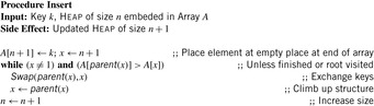
To insert an element into a Heap, we first tentatively place it in the next available leaf. As this might violate the heap property, we restore the heap property by swapping the element with its parent, if the parent's key is larger; then we check for the grandparent key, and so on, until the heap property is valid or the element reaches the root. Thus, Insert needs at most

time. In the array embedding we start with the last unused index n + 1 in array A and place key k into

. Then, we climb up the ancestors until a correct Heap is constructed. An implementation is provided in Algorithm 3.12.

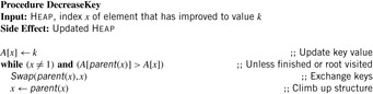
DecreaseKey starts at the node x that has changed its value. This reference has to be maintained with the elements that are stored. Algorithm 3.13 shows a possible implementation.

B9780123725127000031/u03-12-9780123725127.jpg is missing

Algorithm 3.12.

Inserting an element into a Heap.

B9780123725127000031/u03-13-9780123725127.jpg is missing

Algorithm 3.13.

Decreasing the key of an element in a Heap.

To extract the minimum key is particularly easy: It is always stored at the root. However, we have to delete it and guarantee the heap property afterward. First, we tentatively fill the gap at the root with the last element on the bottom level of the tree. Then we restore the heap property using two comparisons per node while going down. This operation is referred to as SiftDown. That is, at a node we determine the minimum of the current key and that of the children; if the node is actually the minimum of the three, we are done, otherwise it is exchanged with the minimum, and the balancing continues at its previous position. Hence, the running time for DeleteMin is again

in the worst-case. The implementation is displayed in Algorithm 3.14. Different SiftDown procedures are known: (1) top-down (as in Alg. 3.15); (2) bottom-up (first following the special path of smaller children to the leaf, then sifting up the root element as in Insert ); or (3) with binary search (on the special path).

B9780123725127000031/u03-14-9780123725127.jpg is missing

Algorithm 3.14.

Extracting the minimum element from a Heap.

B9780123725127000031/u03-15-9780123725127.jpg is missing

Algorithm 3.15.

Rearrange Heap.

An implementation of the priority queue using a Heap leads to an

algorithm for A*, where n(resp. e) is the number of generated problem graph nodes (resp. edges). The data structure is fast in practice if n is small, say a few million elements (an accurate number depends on the efficiency of the implementation).

Pairing Heaps

A Pairing Heap is a heap-ordered (not necessarily binary) self-adjusting tree. The basic operation on a Pairing Heap is pairing, which combines two Pairing Heaps by attaching the root with the larger key to the other root as its left-most child. More precisely, for two Pairing Heaps with respective root values k₁ and k₂, pairing inserts the first as the left-most subtree of the second if

, and otherwise inserts the second into the first as its left-most subtree. Pairing takes constant time and the minimum is found at the root.

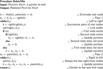
In a multiway tree representation realizing the priority queue operations is simple. Insertion pairs the new node with the root of the heap. DecreaseKey splits the node and its subtree from the heap (if the node is not the root), decreases the key, and then pairs it with the root of the heap. Delete splits the node to be deleted and its subtree, performs a DeleteMin on the subtree, and pairs the resulting tree with the root of the heap. DeleteMin removes and returns the root, and then, in pairs, pairs the remaining trees. Then, the remaining trees from right to left are incrementally paired (see Alg. 3.16).

Since the multiple-child representation is difficult to maintain, the child-sibling binary tree representation for Pairing Heaps is often used, in which siblings are connected as follows. The left link of a node accesses its first child, and the right link of a node accesses its next sibling, so that the value of a node is less than or equal to all the values of nodes in its left subtree. It has been shown that in this representation Insert takes O (1) and DeleteMin takes

amortized, and DecreaseKey takes at least

and at most

steps.

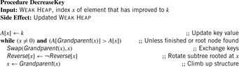
Weak Heaps

A Weak Heap is obtained by relaxing the Heap requirements. It satisfies three conditions: the key of a node is smaller than or equal to all elements to its right, the root has no left child, and leaves are found on the last two levels only.

The array representation uses extra bits Reverse

. The location of the left child is located at

and the right child is found at

. By flipping Reverse

the locations of the left child and the right child are exchanged. As an example take

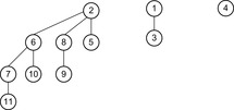
and

as an array representation of a Weak Heap. Its binary tree equivalent is shown in Figure 3.7.

B9780123725127000031/f03-07-9780123725127.jpg is missing

Figure 3.7

Example of a Weak Heap. Reflected nodes are shown in gray.

B9780123725127000031/u03-16-9780123725127.jpg is missing

Algorithm 3.16.

Rearrange Pairing Heap.

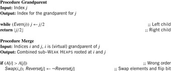
The function Grandparent is defined as

in case i is a left child, and

if i is a right one. In a Weak Heap,

refers to the index of the deepest element known to be smaller than or equal to the one at i. An illustration is given in Figure 3.8.

Figure 3.8

Grandparent relationship in a Weak Heap indicated using dashed arrows.

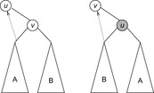
Let node v be the root of a balanced tree T and let node u with the left subtree of T and v with the right subtree of T each form a Weak Heap. Merging u and v yields a new Weak Heap. If

then the tree with root u and right child v is a Weak Heap. If, however,

we swap

with

and reflect the subtrees in T(see Fig. 3.9, right). Algorithm 3.17 provides the pseudo-code implementation for Merge and Grandparent.

B9780123725127000031/f03-09-9780123725127.jpg is missing

Figure 3.9

Merging operation in a Weak Heap.

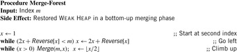
To restore the Weak Heap all subtrees corresponding to grandchildren of the root are combined. Algorithm 3.18 shows the implementation of this Merge-Forest procedure. The element at position m serves as a root node. We traverse the grandchildren of the root in which the second largest element is located. Then, in a bottom-up traversal, the Weak Heap property is restored by a series of Merge operations.

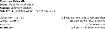
For DeleteMin we restore the Weak Heap property after exchanging the root element with the last one in the underlying array. Algorithm 3.19 gives an implementation.

To construct a Weak Heap from scratch all nodes at index i for decreasing i are merged to their grandparents, resulting in the minimal number of n − 1 comparisons.

B9780123725127000031/u03-17-9780123725127.jpg is missing

Algorithm 3.17.

Implementation of different subroutines for Weak Heaps.

B9780123725127000031/u03-18-9780123725127.jpg is missing

Algorithm 3.18.

Restoration of Weak Heaps.

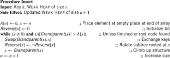
For Insert given a key k, we start with the last unused index x in array A and place k into

. Then we climb up the grandparents until the Weak Heap property is satisfied (see Alg. 3.20). On the average, the path length of grandparents from a leaf node to a root is approximately half of the depth of the tree.

B9780123725127000031/u03-19-9780123725127.jpg is missing

Algorithm 3.19.

Extracting the minimum element from a Weak Heap.

B9780123725127000031/u03-20-9780123725127.jpg is missing

Algorithm 3.20.

Inserting an element into a Weak Heap.

For the DecreaseKey operation we start at the node x that has changed its value. Algorithm 3.21 shows an implementation.

Fibonacci Heaps

A Fibonacci Heap is an involved data structure with a detailed presentation that exceeds the scope of this book. In the following, therefore, we only motivate Fibonacci Heaps.

Intuitively, Fibonacci Heaps are relaxed versions of Binomial Queues, which themselves are extensions to Binomial Trees. A Binomial Tree B_n is a tree of height n with 2ⁿ nodes in total and

nodes in depth i. The structure of B_n is found by unifying 2-structure

, where one is added as an additional successor to the second.

Binomial Queues are unions of heap-ordered Binomial Trees. An example is shown in Figure 3.10. Tree B_i is represented in queue Q if the i th bit in the binary representation of n is set. The partition of a Binomial Queue structure Q into trees B_i is unique as there is only one binary representation of a given number. Since the minimum is always located at the root of one B_i, operation Min takes

time. Binomial Queues Q₁ and Q₂ of sizes n₁ and n₂ are meld by simulating binary addition of n₁ and n₂. This corresponds to a parallel scan of the root lists of Q₁ and Q₂. If

then meld can be performed in time

. Having to meld the queues

and

leads to a queue

B9780123725127000031/u03-21-9780123725127.jpg is missing

Algorithm 3.21.

Decreasing the key of an element in a Weak Heap.

Binomial Queues are themselves priority queues. Operations Insert and DeleteMin both use procedure meld as a subroutine. The former creates a tree B₀ with one element, and the latter extracts tree B_i containing the minimal element and splits it into its subtrees

. In both cases the resulting trees are merged with the remaining queue to perform the update. DecreaseKey for element v updates the Binomial Tree B_i in which v is located by propagating the element change bottom-up. All operations run in

A Fibonacci Heap is a collection of heap-ordered Binomial Trees, maintained in the form of a circular doubly linked unordered list of root nodes. In difference to Binomial Queues, more than one Binomial Tree of rank i may be represented in one Fibonacci Heap. Consolidation traverses the linear list and merges trees of the same rank (each rank is unique). For this purpose, an additional array is devised that supports finding the trees of the same rank in the root list. The minimum element in a Fibonacci Heap is accessible in O (1) time through a pointer in the root list. Insert performs a meld operation with a singleton tree.

B9780123725127000031/f03-10-9780123725127.jpg is missing

Figure 3.10

Example of a Binomial Queue.

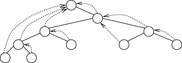
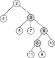
For the critical operation consolidate (see Algorithm 3.22) a node is marked if it loses a child. Before it is marked twice, a cut is performed, which separates the node from its parent. The subtree of the node is inserted in the root list (where the node becomes unmarked again). The cut may cascade as it is propagated to the parent node. An example for a cascading cut is shown in Figure 3.11. Nodes with the keys 3, 6, and 8 are already marked. Now we decrease the key 9 to 1, so that 3, 6, and 8 will lose their second child.

B9780123725127000031/u03-22-9780123725127.jpg is missing

Algorithm 3.22.

Consolidation with bitvectors and heuristic factor in a Fibonacci Heap.

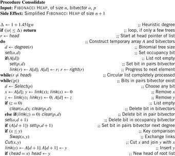
DecreaseKey performs the update on the element in the heap-ordered tree. It removes the updated node from the child list of its parent and inserts it into the root list while updating the minimum. DeleteMin extracts the minimum and includes all subtrees into the root list and consolidates it.

B9780123725127000031/f03-11-9780123725127.jpg is missing

Figure 3.11

Cascading cut in heap-ordered tree.

A heuristic parameter can be set to call consolidation less frequently. Moreover, a bitvector can improve the performance of consolidation, as it avoids additional links and faster access to the trees of the same rank to be merged. In an eager variant Fibonacci heaps maintain the consolidation heap store at any time.

Relaxed Weak Queues

Relaxed Weak Queues are worst-case efficient priority queues, by means that all running times of Fibonacci Heaps are worst-case instead of amortized.

Weak Queues contribute to the observation that Perfect Weak Heaps inherit a one-to-one correspondence to Binomial Queues by only taking edges that are defined by the Grandparent relation. Note that in Perfect Weak Heaps the right subtree of the root is a complete binary tree. A Weak Queue stores n elements and is a collection of disjoint (nonembedded) Perfect Weak Heaps based on the binary representation of

. In its basic form, a Weak Queue contains a Perfect Weak Heap H_i of size 2_i if and only if

Relaxed Weak Queues relax the requirement of having exactly one Weak Heap of a given rank in the Weak Queue and allow some inconsistent elements that violate the Weak Heap property. A structure (of logarithmic size) called the heap store maintains Perfect Weak Heaps of the same rank similar to Fibonacci Heaps. At most two heaps per rank suffice to efficiently realize injection and ejection of the heaps. To keep the worst-case complexity bounds, merging Weak Heaps of the same rank is delayed by maintaining the following structural property on the sequence of numbers of Perfect Weak Heaps of the same rank.

The rank sequence

is regular if any digit 2 is preceded by a digit 0, possibly having some digits 1 in between. A subsequence of the form

is called a block. That is, every digit 2 must be part of a block, but there can be digits, 0's and 1's, that are not part of a block. For example, the rank sequence (1011202012) contains three blocks. For injecting a Weak Heap, we join the first two Weak Heaps that are of the same size, if there are any. They are found by scanning the rank sequence. For O (1) access, a stack of pending joins, the so-called join schedule implements the rank sequence of pending joins. Then we insert the new Weak Heap, which will preserve the regularity of the rank sequence. For ejection, the smallest Weak Heap is eliminated from the heap sequence and, if this Perfect Weak Heap forms a pair with some other Perfect Weak Heap, the top of the join schedule is also popped.

To keep the complexity for DecreaseKey constant, resolving Weak Heap order violations is also delayed. The primary purpose of a node store is to keep track and reduce the number of potential violation nodes at which the key may be smaller than the key of its grandparent. A node that is a potential violation node is marked. A marked node is tough if it is the left child of its parent and also the parent is marked. A chain of consecutive tough nodes followed by a single nontough marked node is called a run. All tough nodes of a run are called its members; the single nontough marked node of that run is called its leader. A marked node that is neither a member nor a leader of a run is called a singleton. To summarize, we can divide the set of all nodes into four disjoint node type categories: unmarked nodes, run members, run leaders, and singletons.

A pair (type, height) with (type) being either unmarked, member, leader, or singleton and (height) being a value in

denotes the state of a node. Transformations induce a constant number of state transitions. A simple example of such a transformation is a join, where the height of the new root must be increased by one. Other operations are cleaning, parent, sibling, and pair transformations (see Fig. 3.12). A cleaning transformation rotates a marked left child to a marked right one, provided its neighbor and parent are unmarked. A parent transformation reduces the number of marked nodes or pushes the marking one level up. A sibling transformation reduces the markings by eliminating two markings in one level, while generating a new marking one level up. A pair transformation has a similar effect, but also operates on disconnected trees.

All transformations run in constant time. The node store consists of different list items containing the type of the node marking, which can either be a fellow, a chairman, a leader, or a member of a run, where fellows and chairmen refine the concept of singletons. A fellow is a marked node, with an unmarked parent, if it is a left child. If more than one fellow has a certain height, one of them is elected a chairman. The list of chairmen is required for performing a singleton transformation. Nodes that are left children of a marked parent are members, while the parent of such runs is entitled the leader. The list of leaders is needed for performing a run transformation.

B9780123725127000031/f03-12-9780123725127.jpg is missing

Figure 3.12

Primitives used in a λ-reduction: (a) cleaning transformation, (b) parent transformation, (c) sibling transformation, and (d) pair transformation.

The four primitive transformations are combined to a λ-reduction, which invokes either a singleton or run transformation (see Alg. 3.23). A singleton transformation reduces the number of markings in a given level by one, not producing a marking in the level above; or it reduces the number of markings in a level by two, producing a marking in the level above. A similar observation applies to a run transformation, so that in both transformations the number of markings is reduced by at least one in a constant amount of work and comparisons. A λ-reduction is invoked once for each DecreaseKey operation. It invokes either a singleton or a run transformation and is enforced, once the number of marked nodes exceeds

Table 3.1 measures the time in μ-seconds (for each operation) for inserting n integers (randomly assigned to values from n to 2n − 1). Next, their values are decreased by 10 and then the minimum element is deleted n times. (The lack of results in one row is due to the fact that Fibonacci Heaps ran out of space.)

**Table 3.1** Performance of priority queue data structures on n integers.
	n = 25'000'000			n = 50'000'000
	Insert	Dec.Key	Del.Min	Insert	Dec.Key	Del.Min
Relaxed Weak Queues	0.048	0.223	4.38	0.049	0.223	5.09
Pairing Heaps	0.010	0.020	6.71	0.009	0.020	8.01
Fibonacci Heaps	0.062	0.116	6.98	—	—	—
Heaps	0.090	0.064	5.22	0.082	0.065	6.37

B9780123725127000031/u03-23-9780123725127.jpg is missing

Algorithm 3.23.

Reducing number of markings in a Relaxed Weak Queue.

3.2. Hash Tables

Duplicate detection is essential for state space search to avoid redundant expansions. As no access to all states is given in advance, a dynamically growing dictionary to represent sets of states has to be provided. For the Closed list, we memorize nodes that have been expanded and for each generated state we check whether it is already stored. We also have to search for duplicates in the Open list, so another dictionary is needed to assist lookups in the priority queue. The Dictionary problem consists of providing a data structure with the operations Insert, Lookup, and Delete. In search applications, deletion is not always necessary. The slightly easier membership problem neglects any associated information. However, many implementations of membership data structures can be easily generalized to dictionary data structures by adding a pointer. Instead of maintaining two dictionaries for Open and Closed individually, more frequently, the Open and Closed lists are maintained together in a combined dictionary.

There are two major techniques for implementing dictionaries: (balanced) search trees and hashing. The former class of algorithms can achieve all operations in

worst-case time and O (n) storage space, where n is the number of stored elements. Generally, for hashing constant time for lookup operations is required, so we concentrate on hash dictionaries. We first introduce different hash functions and algorithms. Incremental hashing will be helpful to enhance the efficiency of computing hash addresses. In perfect hashing we consider bijective mapping of states to addresses. In universal hashing, we consider a class of hash functions that will be useful for more general perfect hashing strategies. Because memory is a big concern in state space search we will also address memory-saving dictionary data structures. At the end of this section, we show how to save additional space by being imprecise (saying in the dictionary when it is not).

3.2.1. Hash Dictionaries

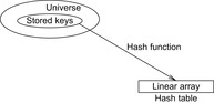
Hashing serves as a method to store and retrieve states

efficiently. A dictionary over a universe

of possible keys is a partial function from a subset

(the stored keys ) to some set I(the associated information). In state space hashing, every state

is assigned to a key k (x), which is a part of the representation that uniquely identifies S. Note that every state representation can be interpreted as a binary integer number. Then not all integers in the universe will correspond to valid states. For simplicity, in the following we will identify states with their keys.

The keys are mapped into a linear array

, called the hash table. The mapping

is called the hash function (see Fig. 3.13). The lack of injectiveness yields address collisions; that is, different states that are mapped to the same table location. Roughly speaking, hashing is all about computing keys and detecting collisions. The overall time complexity for hashing depends on the time to compute the hash function, the collision strategy, and the ratio between the number of stored keys and the hash table size, but usually not on the size of the keys.

B9780123725127000031/f03-13-9780123725127.jpg is missing

Figure 3.13

Basic principle of hashing.

The choice of a good hash function is the central problem for hashing. In the worst-case, all keys are mapped to the same address; for example, for all

we have

, with

. In the best case, we have no collisions and the access time to an element is constant. A special case is that of a fixed stored set R, and a hash table of at least m entries; then a suitable hash function is

with

and

These two extreme cases are more of theoretical interest. In practice, we can avoid the worst-case by a proper design of the hash function.

3.2.2. Hash Functions

A good hash function is one that can be computed efficiently and minimizes the number of address collisions. The returned addresses for given keys should be uniformly distributed, even if the set of chosen keys in S is not, which is almost always the case.

Given a hash table of size m and the sequence

of keys to be inserted, for each pair (k_i, k_j of keys,

, we define a random variable

Then

is the sum of collisions. Assuming a random hash function with uniform distribution, the expected value of X is

Using a hash table of size

, for 1 million elements, we expect about

address collisions.

Remainder Method

If we can extend S to

, then

is the quotient space with equivalence classes

induced by the relation

Therefore, a mapping

with

distributes S on T. For the uniformity, the choice of m is important; for example, if m is even then h (x) is even if and only if x is.

The choice

, for some

, is also not appropriate, since for

we have

This means that the distribution takes only the last w digits into account.

A good choice for m is a prime that does not divide a number

for small j, because

is equivalent to

so that (case +)

that is, keys with same sum of digits are mapped to the same address.

Multiplicative Hashing

In this approach the product of the key and an irrational number ϕ is computed and the fractional part is preserved, resulting in a mapping into

. This can be used for a hash function that maps the key x to

as follows:

One of the best choices for ϕ for multiplicative hashing is

, the golden ratio. As an example take

and

; then

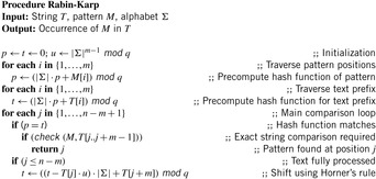
Rabin and Karp Hashing

For incremental hashing based on the idea of Rabin and Karp, states are interpreted as strings over a fixed alphabet. In case no natural string representation exists it is possible to interpret the binary representation of a state as a string over the alphabet {0, 1}. To increase the effectiveness of the method the string of bits may be divided into blocks. For example, a state vector consisting of bytes yields 256 different characters.

The idea of Rabin and Karp originates in matching a pattern string

to a text

. For a certain hash function h, pattern M is mapped to the number h (M), assuming that h (M) fits into a single memory cell and can be processed in constant time. For

the algorithm checks if

. Due to possible collisions, this check is a necessary but not a sufficient condition for a valid match of M and

. To validate that the match is indeed valid in case

, a character-by-character comparison has to be performed.

To compute

in constant time, the value is calculated incrementally—the algorithm takes the known value

into account to determine

with a few CPU operations. The hash function has to be chosen carefully to be suited to the incremental computation; for example, linear hash functions based on a radix number representation such as

are suitable, where q is a prime and the radix r is equal to

Algorithmically, the approach works as follows. Let q be a sufficiently large prime and

. We assume that numbers of size

fit into a memory cell, so that all operations can be performed with single precision arithmetic. To ease notation, we identify characters in Σ with their order. The algorithm of Rabin and Karp as presented in Algorithm 3.24 performs the matching process.

The algorithm is correct due to the following observation.

B9780123725127000031/u03-24-9780123725127.jpg is missing

Algorithm 3.24.

Algorithm of Rabin and Karp.

Theorem 3.1

(Correctness Rabin-Karp) Let the steps ofAlgorithm 3.24be numbered wrt. the loop counter j. At the start of the j th iteration we have

Proof

Certainly,

and inductively we have

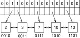
B9780123725127000031/si219.gif is missing

As an example take

and q = 13. Furthermore, let M = 31415 and T = 2359023141526739921. The application of the mapping h is illustrated in Figure 3.14.

Figure 3.14

Example of Rabin-Karp hashing for string matching.

We see h produces collisions. The incremental computation works as follows.

The computation of all hash addresses has a resulting running time of

, which is also the best-case overall running time. In the worst-case, the matching is still of order

, as the example problem of searching

shows.

Incremental Hashing

For a state space search, we have often the case that a state transition changes only a part of the representation. In this case, the computation of the hash function can be executed incrementally. We refer to this approach as incremental state space hashing. The alphabet Σ denotes the set of characters in the string to be hashed. In the state space search, the set Σ will be used for denoting the domain(s) of the state variables.

Take, for example, the Fifteen-Puzzle. With

, a natural vector representation for state u is

, where

means that the tile labeled with l is located at position i, and

is the blank. Because successor generation is fast and Manhattan distance heuristic can be computed incrementally in constant time (using a table addressed by the tile's label

, the tile's move direction

, and the position

of the tile that is being moved), the computational burden is on computing the hash function.

One hash value of a Fifteen-Puzzle state u is

. Let state u′ with representation

be a successor of u. We know that there is only one transposition in the vectors t and t′. Let j be the position of the blank in u and k be the position of the blank in u′. We have

, and for all

, with

, it holds that

. Therefore,

B9780123725127000031/si240.gif is missing

To save time, we may precompute

for each k and l in

. If we were to store

for each value of j, k, and l, we would save another addition. As

and

, we may further substitute the last mod by faster arithmetic operations.

As a particular case, we look at an instance of the Fifteen-Puzzle, where the tile 12 is to be moved downward from its position 11 to position 15. We have

Next we generalize our observations. The savings are larger, when the state vector grows. For the (n² − 1)-Puzzle nonincremental hashing results in

time, whereas in incremental hashing the efforts remain constant. Moreover, incremental hashing is available for many search problems that obey a static vector representation. Hence, we assume that state u is a vector

with u_i in finite domain

Theorem 3.2

(Efficiency of Incremental Hashing) Let I (a) be the set of indices in the state vector that change when applying a, and

. The hash value of v for successor u of v via a given the hash value for u is available in time:

; using an O (k)-size table.

2. O (1); using an

-size table. where

Proof

We define

as the hash function, with

and

for

. For case 1 we store

for all

in a precomputed table, so that

lookups are needed. For case 2 we compute

for all possible actions

. The number of possible actions is bounded by

, since at most

indices may change to at most

different values.

Note that the number of possible actions is much smaller in practice. The effectiveness of incremental hashing relies on two factors: on the state vector's locality (i.e., how many state variables are affected by a state transition) and on the node expansion efficiency (i.e., the running time of all other operations to generate one successor). In the Rubik's Cube, exploiting locality is limited. If we represent position and orientation of each subcube as a number in the state vector, then for each twist, 8 of the 20 entries will be changed. In contrast, for Sokoban the node expansion efficiency is small; as during move execution, the set of pushable balls has to be determined in linear time to the board layout, and the (incremental) computation of the minimum matching heuristic requires at least quadratic time in the number of balls.

For incremental hashing the resulting technique is very efficient. However, it can also have drawbacks, so take care. For example, as with ordinary hashing, the suggested schema induces collisions, which have to be resolved.

Universal Hash Functions

Universal hashing requires a set of hash functions to have on average a good distribution for any subset of stored keys. It is the basis for FKS and cuckoo hashing and has a lot of nice properties. Universal hashing is often used in a state space search, when restarting a randomized incomplete algorithm with a different hash function.

Let

be the set of hash addresses and

be the set of possible keys. A set of hash function H is universal, if for all

The intuition in the design of universal hash functions is to include a suitable random number generator inside the hash computation. For example, the Lehmer generator refers to linear congruences. It is one of the most common methods for generating random numbers. With respect to a triple of constants a, b, and c a sequence of pseudo-random numbers x_i is generated according to the recursion

Universal hash functions lead to a good distribution of values on the average. If h is drawn randomly from H and S is the set of keys to be inserted in the hash table, the expected cost of each Lookup, Insert, and Delete operation is bounded by

. We give an example of a class of universal hash functions. Let

, p be prime with

. For

, define

Then

is a set of universal hash functions. As an example, take m = 3 and p = 5. Then we have 20 functions in H:

B9780123725127000031/si279.gif is missing

all taken mod 5 mod 3. Hashing 1 and 4 yields the following address collisions:

B9780123725127000031/si280.gif is missing

To prove that H is universal, let us look at the probability that two keys

are mapped to locations r and s by the inner part of the hash function,

This means that

, which has exactly one solution

since

is a field (we needed

to ensure that

). Value r cannot be equal to s, since this would imply

, contrary to the definition of the hash function. Therefore, we now assume

. Then there is a 1 in

chance that a has the right value. Given this value of a, we need

, and there is a

chance that b gets this value. Consequently, the overall probability that the inner function maps x to r and y to s is

Now, the probability that x and y collide is equal to this

, times the number of pairs

such that

. We have p choices for r, and subsequently at most

choices for s(the −1 is for disallowing s = r). Using

for integers v and w, the product is at most

Putting this all together, we obtain for the probability of a collision between x and y,

Perfect Hash Functions

Can we find a hash function h such that (besides the efforts to compute the hash function) all lookups require constant time? The answer is yes—this leads to perfect hashing. An injective mapping of R with

is called a perfect hash function; it allows an access without collisions. If n = m we have a minimal perfect hash function. The design of perfect hashing yields an optimal worst-case performance of O (1) accesses. Since perfect hashing uniquely determines an address, a state S can often be reconstructed given h (S).

If we invest enough space, perfect (and incremental) hash functions are not difficult to obtain. In the example of the Eight-Puzzle for a state u in vector representation

we may choose

for

different hash addresses (equivalent to about 46 megabytes space). Unfortunately, this approach leaves most hash addresses vacant. A better hash function is to compute the rank of the permutation in some given ordering, resulting in 9! states or about 44 kilobytes.

Lexicographic Ordering

The lexicographic rank of permutation π (of size N) is defined as

where the coefficients d_i are called the inverted index or factorial base.

By looking at a permutation tree it is easy to see that such a hash function exists. Leaves in the tree are all permutations and at each node in level i, the i th vector value is selected, reducing the range of available values in level i + 1. This leads to an

algorithm. A linear algorithm for this maps a permutation to its factorial base

with d_i being equal to t_i minus the number of elements t_j,

that are smaller than t_i; that is;

with the number of inversions c_i being set to

. For example, the lexicographic rank of permutation

is equal to

, corresponding to

and

. The values c_i are computed in linear time using a table lookup in a

-size table T. In the table T we store the number of ones in the binary representation of a value,

with

. For computing the hash value, while processing vector position t_i we mark bit t_i in bitvector x(initially set to 0). Thus, x denotes the tiles we have seen so far and we can take

as the value for c_i. Since this approach consumes exponential space, time-space trade-offs have been discussed.

For the design of a minimum perfect hash function of the sliding-tile puzzles we observe that in a lexicographic ordering every two successive permutations have an alternating signature (parity of the number of inversions) and differ by exactly one transposition. For minimal perfect hashing a (n² − 1)-Puzzle state to

we consequently compute the lexicographic rank and divide it by 2. For unranking, we now have to determine which one of the two uncompressed permutations of the puzzle is reachable. This amounts to finding the signature of the permutation, which allows us to separate solvable from insolvable states. It is computed as

. For example, with

we have

B9780123725127000031/u03-25-9780123725127.jpg is missing

Algorithm 3.25.

Rank operation for permutations.

There is one subtle problem with the blank. Simply taking the minimum perfect hash value for the alternation group in

does not suffice, since swapping a tile with the blank does not necessarily toggle the solvability status (e.g., it may be a move). To resolve this problem, we partition state space along the position of the blank. Let

denote the sets of blank-projected states. Then each B_i contains

elements. Given index i and the rank inside B_i, it is simple to reconstruct the state.

Myrvold Ruskey Ordering

We next turn to alternative permutation indices proposed by Myrvold and Ruskey. The basic motivation is the generation of a random permutation according to swapping

with

, where r is a random number uniformly chosen in

, and i decreases from N − 1 down to 1.

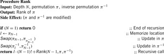
One (recursive) algorithm Rank is shown in Algorithm 3.25. The permutation π and its inverse

are initialized according to the permutation, for which a rank has to be determined.

The inverse

of π can be computed by setting

, for all

. Take as an example permutation

. Then its rank is

. This unrolls to

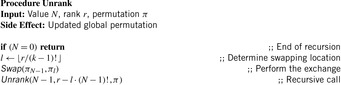
. It is also possible to compile a rank back into a permutation in linear time. The inverse procedure Unrank, initialized with the identity permutation, is shown in Algorithm 3.26. The depth value N is initialized with the size of the permutation, and the rank r is the value computed with Algorithm 3.25. (As a side effect, if the algorithm is terminated at the N th step, the positions

hold a random l-permutation of the numbers

Algorithm 3.27 shows another (in this case nonrecursive) unrank algorithm proposed by Myrvold and Ruskey. It also detects the parity of the number of inversions (the signature of the permutation) efficiently and fits to the ranking function in Algorithm 3.28. All permutations of size N = 4 together with their signature and ranked according to the two approaches are listed in Table 3.2.

**Table 3.2** Myrvold and Ruskey 's perfect permutation hash functions.
Index	Unrank (Alg. 3.26)	Signature	Unrank (Alg. 3.27)	Signature
0	(2,1,3,0)	0	(1,2,3,0)	0
1	(2,3,1,0)	1	(3,2,0,1)	0
2	(3,2,1,0)	0	(1,3,0,2)	0
3	(1,3,2,0)	1	(1,2,0,3)	1
4	(1,3,2,0)	1	(2,3,1,0)	0
5	(3,1,2,0)	0	(2,0,3,1)	0
6	(3,2,0,1)	1	(3,0,1,2)	0
7	(2,3,0,1)	0	(2,0,1,3)	1
8	(2,0,3,1)	1	(1,3,2,0)	1
9	(0,2,3,1)	0	(3,0,2,1)	1
10	(3,0,2,1)	0	(1,0,3,2)	1
11	(0,3,2,1)	1	(1,0,2,3)	0
12	(1,3,0,2)	0	(2,1,3,0)	1
13	(3,1,0,2)	1	(2,3,0,1)	1
14	(3,0,1,2)	0	(3,1,0,2)	1
15	(0,3,1,2)	1	(2,1,0,3)	0
16	(1,0,3,2)	1	(3,2,1,0)	1
17	(0,1,3,2)	0	(0,2,3,1)	1
18	(1,2,0,3)	1	(0,3,1,2)	1
19	(2,1,0,3)	0	(0,2,1,3)	0
20	(2,0,1,3)	1	(3,1,2,0)	0
21	(0,2,1,3)	0	(0,3,2,1)	0
22	(1,0,2,3)	0	(0,1,3,2)	0
23	(0,1,2,3)	1	(0,1,2,3)	1

Theorem 3.3

(Myrvold-Ruskey Permutation Signature) Given the Myrvold-Ruskey rank (as computed byAlg. 3.28), the signature of a permutation can be computed in O (N) time withinAlgorithm 3.27.

Proof

In the unrank function we always have N − 1 element exchanges. For swapping two elements u and v at respective positions i and j with

we count

transpositions:

. As

, each transposition either increases or decreases the parity of the number of inversion, so that the parity for each iteration toggles. The only exception is if

, where no change occurs. Hence, the sign of the permutation can be determined by executing the Myrvold-Ruskey algorithm in O (N) time.

B9780123725127000031/u03-26-9780123725127.jpg is missing

Algorithm 3.26.

Unrank operation for permutations.

B9780123725127000031/u03-27-9780123725127.jpg is missing

Algorithm 3.27.

Recursion-free unranking and signature computation.

Theorem 3.4

(Compression of Alternation Group) Let π (i) denote the value returned by the Myrvold and Ruskey's Unrank function (Alg. 3.28) for index i. Then π (i) matches

except for transposing π₀ and π₁.

Proof

The last call for

in Algorithm 3.27 is

, which resolves to either

. Only the latter one induces a change. If

denote the indices of

in the iterations

of Myrvold and Ruskey's Unrank function, then

, which is 1 for

and 0 for

3.2.3. Hashing Algorithms

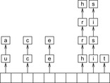
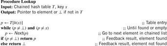
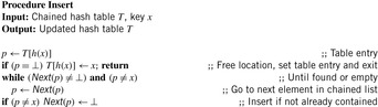
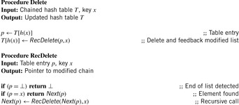
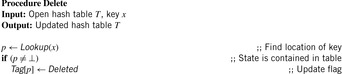
There are two standard options for dealing with colliding items: chaining or open addressing. In hashing with chaining, keys x are kept in linked overflow lists. The dictionary operations Lookup, Insert, and Delete amount to computing h (x) and then performing pure list manipulations in

. Their pseudo-code implementation is provided in Algorithm 3.29, Algorithm 3.30 and Algorithm 3.31. They assume a null pointer ⊥ and a link Next to the successor in the chained list. Operations Insert and Delete suggest a call to Lookup prior to their invocation to determine whether or not the element is contained in the hash table. An example for hashing the characters in heuristic search in a table of 10 elements with respect to their lexicographical order modulo 10 is depicted in Figure 3.15.

B9780123725127000031/f03-15-9780123725127.jpg is missing

Figure 3.15

Hashing the characters of the term heuristic search with chaining.

B9780123725127000031/u03-28-9780123725127.jpg is missing

Algorithm 3.28.

Recursion-free ranking operation for permutations.

B9780123725127000031/u03-29-9780123725127.jpg is missing

Algorithm 3.29.

Searching a chained hash table.

B9780123725127000031/u03-30-9780123725127.jpg is missing

Algorithm 3.30.

Inserting an element into a chained hash table.

B9780123725127000031/u03-31-9780123725127.jpg is missing

Algorithm 3.31.

Deleting an element from a chained hash table.

Hashing with open addressing integrates the colliding elements at free locations in the hash table; that is, if

is occupied, it searches for an alternative location for x. Searching a key x starts at h (x) and continues in the probing sequence until either x or an empty table entry is found. When deleting an element, some keys may have to be moved back to fill the hole in the lookup sequence.

The linear probing strategy considers

for

. In general, we have the sequence

for probing function

There is a broad spectrum of suitable probing sequences, for example,

B9780123725127000031/si361.gif is missing

where r_x is a random number depending on x, and h′ is a second function, which determines the step size of the probing sequence in double hashing.

B9780123725127000031/u03-32-9780123725127.jpg is missing

Algorithm 3.32.

Searching an element in an open hash table.

To exploit the whole table,

, …,

, and

should be a permutation of

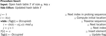
An implementation of the procedure Lookup for a generic probing function s is provided in Algorithm 3.32. The implementation assumes an additional array Tag that associates one of the values Empty, Occupied, and Deleted with each element. Deletions (see Alg. 3.33) are handled by setting the Deleted tag for the cell of the deleted key. Lookups skip over deleted cells, and insertions (see Alg. 3.34) overwrite them.

When the hash table is nearly full, unsuccessful searches lead to long probe sequences. An optimization is ordered hashing, which maintains all probe sequences sorted. Thus, we can abort a Lookup operation as soon as we reach a larger key in the probe sequence. The according algorithm for inserting a key x is depicted in Algorithm 3.35. It consists of a search phase and an insertion phase. First, the probe sequence is followed up to a table slot that is either empty or contains an element that is larger than x. The insertion phase restores the sorting condition to make the algorithm work properly. If x replaces an element

, the latter has to be reinserted into its respective probe sequence, in turn. This leads to a sequence of updates that end when an empty bin is found. It can be shown that the average number of probes to insert a key into the hash table is the same as in ordinary hashing.

B9780123725127000031/u03-33-9780123725127.jpg is missing

Algorithm 3.33.

Inserting an element into an open hash table.

B9780123725127000031/u03-34-9780123725127.jpg is missing

Algorithm 3.34.

Deleting an element from an open hash table.

B9780123725127000031/u03-35-9780123725127.jpg is missing

Algorithm 3.35.

Inserting an element for ordered hashing.

For a hash table of size m that stores n keys, the quotient

is called the load factor. The load factor crucially determines the efficiency of hash table operations. The analysis assumes uniformness of h; that is,

for all

and

. Under this precondition, the expected number of memory probes for insertion and unsuccessful lookup is

B9780123725127000031/si372.gif is missing

Thus, for any

, in terms of number of probes we obtain the following rank order: ideal hashing, chained hashing, double hashing, quadratic probing, and linear probing. The order of the last four methods is true for any α.

Although chaining scores quite favorably in terms of memory probes, the comparison is not totally fair, since it dynamically allocates memory and uses extra linear space to store the pointers.

FKS Hashing Scheme

With a hash function h of a class H of universal hash functions, we can easily obtain constant lookup time if we don't mind spending a quadratic amount of memory. Say we allocate a hash table of size

. Since there are

pairs in R, each with a chance

of colliding with each other, the probability of a collision in the hash table is bounded by

. In other words, the chance of drawing a perfect hash function for the set of stored keys is

. While for each given hash function there is a worst set of stored keys that maps all of them into the same bin, the crucial element of the algorithm is a randomized rehashing: If the chosen h actually leads to a collision, just try again with another hash function drawn with uniform probability from H.

Perfect hashing has important advances in storing and retrieving information in the visited list and, equally important, for fast lookup of pattern databases (see Ch. 4). The apparent question for practical search is whether memory consumption for perfect hashing can be reduced. The so-called FKS hashing scheme (named after the initials of the inventors Fredman, Komlòs, and Szemerèdi) ended a long dispute in research about whether it is also possible to achieve constant access time with a linear storage size of O (n). The algorithm uses a two-level approach: First, hash into a table of size n, which will produce some collisions, and then, for each resulting bin, rehash it as just described, squaring the size of the hash bucket to get zero collisions.

Denote the subset of elements mapped to bin i as R_i, with

. We will use the property that

(3.1)

This can be seen by noting that

is the total number of ordered pairs that land in the same bin of the table; we have

B9780123725127000031/si382.gif is missing

Using the Markov inequality

with

shows

. Consequently,

Choosing

, this implies that for at least half of the functions

we have

(3.2)

At the second level, we use the same property with the choice of the size of the hash table for R_i,

. Then, for at least half of the functions

we obtain

where n_ij is the number of elements in the second-level bin j of R_i; in other words,

for all j.

So, the total space used is O (n) for the first table (assuming it takes a constant amount of space to store each hash function), plus

for the other tables. For the last equality we used Equation 3.2.

Dynamic Perfect Hashing

Unfortunately, the FKS hashing scheme is only applicable to the static case, where the hash table is created once with a fixed set of keys, and no insertions and deletions are allowed afterward.

Later the algorithm was generalized to allow for update operations. Deletion of an element is handled simply by tagging it, and subsequently ignoring tagged keys, overwriting them later.

A standard doubling strategy is used to cope with a growing or shrinking number of stored elements. Every time that a predetermined maximum number of update operations has occurred, the structure is recreated from scratch in the same way as in the static case, but slightly larger than necessary to accommodate future insertions. More precisely, it is planned for a maximum capacity of

, where n is the number of currently stored keys. The top-level hash function contains s (m) bins, which is defined as an O (n) function. Each second-level bin is allocated for a capacity m_i of twice as many elements in it; that is, if n_i keys fall into bin i, its size is chosen as

, with

. The resulting new structure will be used subsequently for at most

update operations.

Before this maximum update count is reached, an insert operation first tries to insert an element according to the given structure and hash functions; this is possible if Equation 3.2 is still valid, the bin i the element is mapped to has some spare capacity left (i.e.,

), and the position within bin i assigned by the second-level hash function is empty. If only the last condition doesn't hold, bin i is reorganized by randomly drawing a new second-level hash function. If

, the bin's capacity is doubled (from m_i to

) prior to reorganization. If, on the other hand, Equation 3.2 is violated, a new top-level hash function has to be selected, and hence the whole structure must be recreated.

It can be shown that this scheme uses O (n) storage; Lookup and Delete are executed in constant worst-case time, whereas Insert runs in constant amortized expected time.

Cuckoo Hashing

The FKS hashing is involved and it is unclear whether the approach can be made incremental. For the first-level hash function this is possible, but for the selection of a universal hash function for each bucket we lack an appropriate answer.

Therefore, we propose an alternative conflict strategy. Cuckoo hashing implements the dictionary with two hash tables, T₁ and T₂, and two different hash functions, h₁ and h₂. Each key, k, is contained either in

or in

. Algorithm 3.36 provides a pseudo-code implementation for searching a key. If an item produces a collision in the first table the detected synonym is deleted and inserted into the other table. Figure 3.16 gives an example—arrows point to the alternative bucket in the other hash table. If D is hashed into the first hash table where it preempts C, then C needs to go into the second hash table where it preempts B, and B needs to go into the first hash table where it found an empty location. During the insertion process the arrows have to be inverted. That is, B that has been moved to the first table points to C in the second table, and C that has been moved to the second table now points to the inserted element D in the first table.

B9780123725127000031/f03-16-9780123725127.jpg is missing

Figure 3.16

A successful insertion of an element via cuckoo hashing.

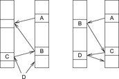
There is a small probability that the cuckoo process may not terminate at all and loop forever; Figure 3.17 gives an example. If D is hashed into the first hash table where it preempts C, then C needs to go into the second hash table where it preempts A, A needs to go into the first hash table where it preempts E, E needs to go into the second hash table where it preempts B, B needs to go into the first hash table where it preempts D, D needs to go into the second hash table where it preempts G, G needs to go into the first hash table where it preempts F, F needs to go into the second hash table where it preempts D, D needs to go into the first hash table where it preempts B, and so on. The analysis shows that such a situation is rather unlikely, so that we can pick fresh hash functions and rehash the entire structure after a fixed number t of failures. Algorithm 3.37 provides an implementation for the insert procedure.

Algorithm 3.36.

Lookup for a key in a cuckoo hash table.

Although reorganization costs linear time it contributes a small amount to the expected runtime. The analysis reveals that if t is fixed appropriately (

for r being the individual hash table sizes and

) the probability of rehash is

. Therefore, rehashing n elements causes no recursive rehash with probability

. As the expected time for inserting one element is constant, the total expected time to reinsert all n elements is O (n). This is also the total expected time for rehashing.

B9780123725127000031/f03-17-9780123725127.jpg is missing

Figure 3.17

An infinite cuckoo process; rehashing is needed.

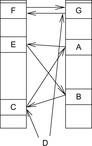
In summary, cuckoo hashing has worst-case constant access time and amortized worst-case insertion time. It is simple to implement and efficient in practice.

B9780123725127000031/u03-37-9780123725127.jpg is missing

Algorithm 3.37.

Inserting a key into a cuckoo hash table.

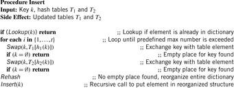
3.2.4. Memory-Saving Dictionaries

The information-theoretic lower bound on the number of bits required to store an arbitrary subset of size n of a universe of size N is

, since we have to be able to represent all possible combinations of selecting n values out of the N. Using Stirling's approximation and defining

, we obtain

with an error less than

, where e is Euler's constant. Alternatively, using

we can approximate the logarithm by two corresponding integrals. If we properly bias the integral limits we can be sure to compute a lower bound

For the case of dynamic dictionaries (where insertions and deletions are fully supported), we want to be able to maintain subsets of varying size, say, of zero up to a maximum of n elements. This results in a minimum number of

bits. For

(which is usually the case for nontrivial search problems) we have

The correctness follows from the property of binomial coefficients

for

. We are only interested in the logarithms, so we conclude

Obviously in this restricted range it is sufficient to concentrate on the last binomial coefficient. The error in our estimate is at most one bit. At the end, as we look at the logarithms, the dynamic case is not much different from the static case.

If N is large compared to n, listing all elements, for example, in a hash table comes close to the information-theoretic minimum number of bits B. In the other border case, for small r it is optimal to list the answers, for example, in the form of a bitvector of size N. The more difficult part is to find appropriate representations for intermediate sizes.

Suffix Lists

Given B bits of memory, for space-efficient state storage we want to maintain a dynamically evolving visited list closed under inserts and membership queries. For the ease of presentation, the entries of Closed are integers from

. Using hashing with open addressing, the maximal size of Closed nodes m is limited to

, since

bits are required to encode a state. A gain is only to be expected if we can exploit redundancies in the state vector set. In the following we describe a simple but very space-efficient approach with small update and query times.

Let

be the binary representation of an element

from the set Closed. We split

in p high bits and

low bits. Furthermore,

denotes the prefix of

and

stands for the suffix of

A Suffix Tree list data structure consists of a linear array P of size 2^p bits and of a two-dimensional array L of size

bits. The basic idea of a Suffix Tree list is to store a common prefix of several entries as a single bit in P, whereas the distinctive suffixes form a group within L. P is stored as a bit array. L can hold several groups with each group consisting of a multiple of

bits. The first bit of each

-bit row in L serves as a group bit. The first s-bit suffix entry of a group has group bit one, and the other elements of the group have group bit zero. We place the elements of a group together in lexicographical order (see Fig. 3.18).

First, we compute

, which gives us the search position in the prefix array P. Then we simply count the number of ones in P starting from position

until we reach

. Let z be this number. Finally, we search through L until we have found the z th suffix of L with group bit one. If we have to perform a membership query we simply search in this group. Note that searching a single entry may require scanning large areas of main memory.

B9780123725127000031/f03-18-9780123725127.jpg is missing

Figure 3.18

Example for a Suffix List with p = 4 and s= 3.

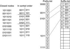
To insert entry u we first search the corresponding group as described earlier. In case u opens a new group within L this involves setting group bits in P and L. The suffix of u is inserted in its group while maintaining the elements of the group sorted. Note that an insert may need to shift many rows in L to create space at the desired position. The maximum number m of elements that can be stored in B bits is limited as follows: We need

bits for P and

bits for each entry of L. Hence, we choose p so that r is maximal subject to

For

the space requirement for both P and the suffixes in L is small enough to guarantee

We now show how to speed up the operations. When searching or inserting an element u we have to compute z to find the correct group in L. Instead of scanning potentially large parts of P and L for each single query we maintain checkpoints, one-counters, to store the number of ones seen so far. Checkpoints are to lie close enough to support rapid search but must not consume more than a small fraction of the main memory. For

we have

for both arrays, so

bits are sufficient for each one-counter.

Keeping one-counters after every

entries limits the total space requirement. Binary search on the one-counters of P now reduces the scan area to compute the correct value of z to

bits.

Searching in L is slightly more difficult because groups could extend over 2^s entries, thus potentially spanning several one-counters with equal values. Nevertheless, finding the beginning and the end of large groups is possible within the stated bounds. As we keep the elements within a group sorted, another binary search on the actual entries is sufficient to locate the position in L.

We now turn to insertions where two problems remain: adding a new element to a group may need shifting large amounts of data. Also, after each insert the checkpoints must be updated. A simple solution uses a second buffer data structure BU that is less space efficient but supports rapid inserts and lookups. When the number of elements in BU exceeds a certain threshold, BU is merged with the old Suffix Tree list to obtain a new up-to-date space-efficient representation. Choosing an appropriate size of BU, amortized analysis shows improved computational bounds for inserts while achieving asymptotically the same order of phases for the graph search algorithm.

Note that membership queries must be extended to BU as well. We implement BU as an array for hashing with open addressing. BU stores at most

elements of size

, for some small constant c₂. As long as there is 10% space left in BU, we continue to insert elements into BU, otherwise BU is sorted and the suffixes are moved from BU into the proper groups of L. The reason not to exploit the full hash table size is again to bound the expected search and insert time within BU to a constant number of tests. Altogether, we can prove the following theorem.

Theorem 3.5

(Time Complexity Suffix Tree list) Searching and inserting n items into a Suffix Tree list under space restriction amounts to a runtime of O (nlgn).

Proof

For a membership query we perform binary searches on numbers of

bits or s bits, respectively. So, to search an element we need

bit operations since

and

Each of the

buffer entries consists of

bits, hence sorting the buffer can be done with

bit operations. Starting with the biggest occurring keys merging can be performed in O (1) memory scans. This also includes updating all one-counters. In spite of the additional data structures we still have

Thus, the total bit complexity for n inserts and membership queries is given by

B9780123725127000031/si457.gif is missing

Assuming a machine word length of

, any modification or comparison of entries with

bits appearing in a Suffix Tree list can be done using O (1) machine operations. Hence, the total complexity reduces to

operations.

The constants can be improved using the following observation: In the case n = (1 + ϵ) ⋅ B, for a small ϵ > 0 nearly half of the entries in P will always be zero, namely those that are lexicographically bigger than the suffix of n itself. Cutting the P array at this position leaves more room for L, which in turn enables us to keep more elements.

Table 3.3 compares a Suffix Tree list data structure with hashing and open addressing. The constants for the Suffix Tree list are chosen so that

, which means that if m elements can be treated, we set aside

bits to speed up internal computations. For hashing with open addressing we also leave 10% of memory free to keep the internal computation time moderate. When using a Suffix Tree list instead of hashing, note that only the ratio between n and B is important.

**Table 3.3** Fractions of n that can be accommodated in a Suffix List and in hashing with open addressing. *Note: n* is the size of the search space to be memorized, and B is the number of bits available for storing the data. The columns denote the maximal portion of the state space that can be stored according to the information theoretical bound, the Suffix List structure, and ordinary hashing according to two practical values of n.
			Hashing
n/B	Upper Bound	Suffix Lists	n = 2²⁰	n = 2³⁰
1.05	33.2%	22.7%	4.3%	2.9%
1.10	32.4%	21.2%	4.1%	2.8%
1.25	24.3%	17.7%	3.6%	2.4%
1.50	17.4%	13.4%	3.0%	2.0%
2.00	11.0%	9.1%	2.3%	1.5%
3.00	6.1%	5.3%	1.5%	1.0%
4.00	4.1%	3.7%	1.1%	0.7%
8.00	1.7%	1.5%	0.5%	0.4%
16.00	0.7%	0.7%	0.3%	0.2%

Hence, the Suffix Tree list data structures can close the memory gap in search algorithms between the best possible and trivial approaches like hashing with open addressing.

3.2.5. Approximate Dictionaries

If we relax the requirements to a membership data structure, allowing it to store a slightly different key set than intended, new possibilities for space reduction arise.

The idea of erroneous dictionaries was first exploited by Bloom. A Bloom Filter is a bitvector v of length m, together with k independent hash functions

. Initially, v is set to zero. To insert a key x, compute

, for all

, and set each

to one. To lookup a key, check the status of

; if it is zero, x is not stored, otherwise continue with

. If all these bits are set, report that x is in the filter. However, since they might have been turned on by different keys, the filter can make false positive errors. Deletions are not supported by this data structure, but they can be incorporated by replacing the bits by counters that are incremented in insertions rather than just set to one.

Bit-State Hashing

For large problem spaces, it can be most efficient to apply a depth-first search strategy in combination with duplicate detection via a membership data structure. Bit-state hashing is a Bloom Filter storage technique without storing the complete state vectors. If the problem contains up to 2³⁰ states and more (which implies a memory consumption of 1GB times state vector size in bytes), it resorts to approximate hashing. Obviously, the algorithm is no longer guaranteed to find a shortest solution (or any solution at all, for that matter). As an illustration of the bit-state hashing idea, Figure 3.19, Figure 3.20 and Figure 3.21 depict the range of possible hash structures: usual hashing with chaining, single-bit hashing, and double-bit hashing.

B9780123725127000031/f03-19-9780123725127.jpg is missing

Figure 3.19

Ordinary hashing with chaining.

Figure 3.20

Single bit-state hashing.

B9780123725127000031/f03-21-9780123725127.jpg is missing

Figure 3.21

Double bit-state hashing.

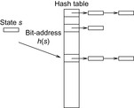
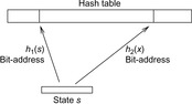
Let n be the number of reachable states and m be the maximal number of bits available. As a coarse approximation for single bit-state hashing with

, the average probability P₁ of a false positive error during the course of the search is bounded by

since the i th element collides with one of the i − 1 already inserted elements with a probability of at most

. For multibit hashing using h(independent) hash functions with the assumption

, the average probability of collision P_h is reduced to

, since i elements occupy at most

addresses,

. In the special case of double bit-state hashing, this simplifies to

An attempt to remedy the incompleteness of partial search is to reinvoke the algorithm several times with different hash functions to improve the coverage of the search tree. This technique, called sequential hashing, successively examines various beams in the search tree (up to a certain threshold depth). In considerably large problems, sequential hashing succeeds in finding solutions (but often returns long paths). As a rough estimate on the error probability we take the following. If in sequential hashing exploration of which the first hash function covers

of the search space, the probability that a state x is not generated in d independent runs is

, such that x is reached with probability

Hash Compaction

To increase the coverage of the search space, further lossy compression techniques have been considered in practice to best exploit the limited amount of memory. Like bit-state hashing, the hash compaction method aims at reducing the memory requirements for the state table. However, it stores a compressed state descriptor in a conventional hash table instead of setting bits corresponding to hash values of the state descriptor in a bitvector. The compression function c maps a state to a b-bit number in

. Since different states can have the same compression, false positive errors can arise. Note, however, that if the probe sequence and the compression are calculated independently from the state, the same compressed state can occur at different locations in the table.

In the analysis, we assume that breadth-first search with ordered hashing using open addressing is applied. Let the goal state s_d be located at depth d, and

be a shortest path to it.

It can be shown that the probability p_k of a false positive error, given that the table already contains k elements, is approximately equal to

(3.3)

where

denotes a harmonic number.

Let k_i be the number of states stored in the hash table after the algorithm has completely explored the nodes in level i. Then there were at most

states in the hash table when we tried to insert s_i. Hence, the probability

that no state on the solution path was omitted is bounded by

If the algorithm is run up to a maximum depth d, it can record the k_i values online and report this lower bound on the omission probability after termination.

To obtain an a priori estimate, knowledge of the depth of the search space and the distribution of the k_i is required. For a coarse approximation, we assume that the table fills up completely (m = n) and that half the states in the solution path experience an empty table during insertion, and the other half experiences the table with only one empty slot. This models (crudely) the typically bell-shaped state distribution over the levels 0,…,d. Assuming further that the individual values in Equation 3.3 are close enough to one to approximate the product by a sum, we obtain the approximation

Assuming, more conservatively, only one empty slot for all states on the solution path would increase this estimate by a factor of two.

Collapse Compression

A related memory-saving strategy is collapse compression. It stores complex state vectors in an efficient way. The main idea is to store different parts of the state space in separate descriptors and represent the actual state as an index to relevant states. Collapse compression is based on the observation that although the number of distinct search states can become very large, the number of distinct parts of the state vector are usually smaller. In contrast, to jointly store the leading part of the state vector, as in Suffix Tree lists, different parts of the state can be shared (across all the visited states that are stored). This is especially important when only small parts of the state vector change and avoids storing the complete vector every time a new state is visited.

Essentially, different components are stored in separate hash tables. Each entry in one of the tables is given a unique number. A whole state vector is then identified by a vector of numbers that refer to corresponding components in the hash tables. This greatly reduces the storage needs for storing the set of already explored states. An illustration of this technique is provided in Figure 3.22. Besides the memory capacity for the state components, collapse compression additionally needs an overall hash table to represent the combined state. The collapsed state vector consists of (hash) IDs for the individual components. Therefore, there is a gain only if the individual state components that are collapsed are themselves complex data structures. Collapse compression can be implemented lossless or lossy.

B9780123725127000031/f03-22-9780123725127.jpg is missing

Figure 3.22

Effect of collapse compression. On the left there is the search tree. On the right, the states have been partitioned in three parts, which are stored individually and jointly addressed with indices. When moving from a to b only the part in the middle of the state vector changes and has to be newly stored.

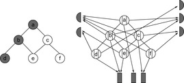
3.3. Subset Dictionaries

The problem of finding an element in a set of elements such that this element is a subset (or a superset) of the query occurs in many search applications; for example, in the matching of a large number of production rules, in the identification of inconsistent subgoals in AI planning, and in finding string completions for constructing or solving crossword puzzles. Moreover, efficiently storing and searching partial information is central to many learning processes. The problem also occurs in search applications that allow the user to search for documents containing a given set of words, and therefore extends the setting in the previous section.

For a state space search the stored sets often correspond to partially specified state vectors (patterns ). As an example, consider the solitaire game Sokoban (see Ch. 1), together with a selection of dead-end patterns. Since every given state is unsolvable, if the dead-end pattern is a subset of it, we want to quickly detect whether or not such a dead-end pattern is present in the data structure (see Ch. 10). We assume the patterns to sets of elements from a certain universe Γ (set of coordinates in Sokoban).

Definition 3.1

(Subset and Containment Query Problem, Subset Dictionary) Let D be a set of n subsets over a universe Γ. The Subset Query (Containment Query) problem asks for any query set

if there is any

with

A subset dictionary is an abstract data structure providing insertion of sets to D while supporting subset and containment queries.

Since p is a subset of q if and only if its complement is a superset of the complement of q, the two query problems are equivalent.

For the Sokoban problem, we have that each board position is an element of Γ. Inserting a pattern amounts to inserting a subset of Γ to the subset dictionary. Subsequently, determining whether or not a state matches a stored pattern is a containment query to the dictionary.

From an implementation point of view we may think of subset dictionaries as hash tables that contain generalized information about sets of problem states. But before diving into implementation issues, we draw another equivalence, which turns out to be essential.

Definition 3.2

(Partial Match) Let * denote a special don't care character that matches every character contained in an alphabet. Given a set D of n vectors over the alphabet Σ, the Partial Match problem asks for a data structure, which for any query

detects if there is any entry p in D such that q matches p.

The application for this problem is to solve approximate matching problems in information retrieval. A sample application is a crossword puzzle dictionary. A query like B*T*R in the Crossword Puzzle would be answered with words like BETTER, BITTER, BUTLER, or BUTTER.

Theorem 3.6

(Equivalence Partial Match and Subset Query Problems) The Partial Match problem is equivalent to the Subset Query problem.

Proof

As we can adjust any algorithm for solving the Partial Match problem to handle binary symbols by using a binary representation, it is sufficient to consider the alphabet

To reduce the Partial Match to the Subset Query problem, we replace each

by a set of all pairs

for all

. Moreover, we replace each query q by a set of all pairs

provided that q is not the don't care symbol ∗. Solving this instance to the subset query problem also solves the Partial Match problem.

To reduce the Subset Query to the Partial Match problem, we replace each database set by its characteristic vector, and replace query set q by its characteristic vector, of which the zeros have been replaced with don't cares.

As the Subset Query is equivalent to the Containment Query problem, the latter one can also be solved by algorithms for the Partial Match. For the sake of simplicity, in the following data structures we restrict the alphabet for the Partial Match problem to {0, 1}.

3.3.1. Arrays and Lists

These problems have two straightforward solutions. The first approach is to store all answers to all possible queries in a (perfect) hash table or array of size 2^m, with

. Query time is O (m) to compute the hash address. For the Containment Query each hash table entry contains a list of sets from the database corresponding to the query (state), which in turn is interpreted as a bitvector. Unfortunately, the memory requirements for this implementation are too large for most practical applications because we have to reserve a table entry for all queries (corresponding to the entire state space).

The list representation with each list item containing one database entry is the other extreme. The storage requirements with O (n) are optimal but searching for a match now corresponds to time O (nm), a term that is also too big for practical applications. In the following, we propose compromises in between storing plain arrays and lists.

3.3.2. Tries

One possible implementation that immediately comes to mind is a Trie, which compares a query string to the set of stored entries. A Trie is a lexicographic search tree structure, in which each node spawns at most

children. The transitions are labeled by

and are mutually exclusive for two successors of a state. Leaf nodes correspond to stored strings. A Trie is a natural and unique representation for a set of strings.

Since inserting and deleting strings in a Trie is simple, in Algorithm 3.38 we consider the traversal of the tree for a search. For notational convenience, we consider the Partial Match problem as introduced earlier. The recursive procedure Lookup is initially invoked with the root of the Trie, the query

with

, and the level 1. The expected sum of nodes examined has been estimated by

, where s is the number of indices specified in a query.

3.3.3. Hashing

An alternative reduction of the space complexity for the array representation is to hash the query sets to a smaller table. The lists in the chained hash table again correspond to database sets. However, the lists have to be searched to filter the elements that match.

A refined implementation of the array approach appropriate for Sokoban is to construct containers L_i of all patterns that share a ball at position i. In the pattern lookup for position u we test whether or not

is empty. Insertion and retrieval time correspond to the sizes

and the individual storage structures for them (e.g., sorted lists, bitvectors, balanced trees).

B9780123725127000031/u03-38-9780123725127.jpg is missing

Algorithm 3.38.

Searching a Trie for a partial match.

B9780123725127000031/u03-39-9780123725127.jpg is missing

Algorithm 3.39.

Searching a hash table for a partial match.

Generalizing the idea for the Partial Match problem leads to the following hashing approach. Let h be the hash function mapping

to the chained hash table. A record p is stored in the list L_j if and only if

For mapping queries q we have to hash all matching elements of

that are covered by q, and define h (q) as the union of all p such that q matches p. The implementation of the Lookup procedure is shown in Algorithm 3.39.

The complexity of computing set h (q) heavily depends on the chosen hash function h. For a balanced hash function, consider the partition of

induced by h; generating blocks

. A hash function is balanced if

is equal to

divided by the hash table size b for all j.

For large alphabets (as in the Crossword Puzzle problem) the hash table size b can be scaled to some value larger than 2^m and letters can be individually mapped. More precisely, we assume an auxiliary hash function h′ that maps Σ to a small set of b bits.

is determined by the concatenation

. A partial match query for queries q like

would be answered by inspecting all

table entries in h (q), where s is the number of fixed bits.

For small alphabets (like the binary case) we have

. One suitable approach is to extract the first

bits of each record as a first hash table index. However, the worst-case behavior can be poor: If none of the bits occurs in the first m positions, then every list must be searched.

To obtain good hash functions also for the worst-case, they have to depend on every input character.

3.3.4. Unlimited Branching Trees

A compromise between the Trie and hash table subset dictionary data structure is an ordered list of tries, called an Unlimited Branching Tree. Insertion is similar to an ordinary Trie insertion with the exception that we maintain a distinctive root for the first element in the sorted representation of the set.

Figure 3.23 displays the Unlimited Branching Tree data structure during the insertion of {1, 2, 3, 4}, {1, 2, 4}, and {3, 4}. To the left of the figure, the first subset generates a new Unlimited Branching Tree. In the middle of the figure, we see that insertion can result in branching. The insertion, which has been executed to the right of the figure, shows that a new Trie is inserted into the root list. The corresponding pseudo code is provided in Algorithm 3.40. The algorithm traverses the root list to detect whether or not a matching root element is present. In case we do not establish a new root element the implementation of the ordinary insert routine for the corresponding Trie (not shown) is called. In case there is no such element, a new one is constructed and added to the list.

B9780123725127000031/f03-23-9780123725127.jpg is missing

Figure 3.23

Evolution of an Generalized Suffix Tree.

The running time of the algorithm is

, where k is the size of the current Trie list and l the size of the sorted set, plus the time

to sort the elements. As with our example it is often the case that all elements are selected from the set

such that the running time is O (n) altogether.

The data structure is designed to solve the Subset Query and the Containment Query problem. In Algorithm 3.41 we show a possible implementation for the latter. First, all root elements matching the query are retrieved. Then the corresponding tries are searched individually for a possible match with the query. As both the query and the stored set are sorted, the match is available in linear time with respect to the query set. The number of root elements that have to be processed can grow considerably and is bounded by the size of the universe Γ.

The worst-case running time of the algorithm is

, where k is the size of the current Trie list and m is the size of the query set plus the time

to sort the elements. If all set elements have been selected from the set

, the worst-case running time is bounded by

B9780123725127000031/u03-40-9780123725127.jpg is missing

Algorithm 3.40.

Inserting a set in an Unlimited Branching Tree.

B9780123725127000031/u03-41-9780123725127.jpg is missing

Algorithm 3.41.

Searching for subsets in an Unlimited Branching Tree.

The matching efforts have been reduced using a data structure from rule-based production systems. The so-called Rete algorithm exploits the fact that the firing of rules, or playing moves as in our case, only changes a few parts of the state, and are of structural similarity, meaning that the same subpattern can occur in multiple rules. The Rete algorithm uses a rooted acyclic-directed graph, the Rete, where the nodes, with the exception of the root, represent patterns, and the edges represent dependencies (the relation ⊆ defined earlier can be directly mapped).

3.4. String Dictionaries

String dictionaries offer substring and superstring queries, and are a specialization of subset dictionaries since substrings and superstrings are consecutive character vectors that do not include gaps. In the following, we study string dictionaries based on Suffix Tree.

A Suffix Tree is a compact trie representation of all suffixes of a given string. The substring information stored at each suffix node is simply given by the indices of the first and the last characters. In the following, the Suffix Tree data structure and its linear-time construction algorithm are explained in detail.

Inserting each suffix of string m in a Trie yields a Suffix Trie. To avoid conflicts at terminal nodes, we append a special character $ to m. For notational convenience, in the following this tag is commonly interpreted as an integral part of m. An example of a Suffix Trie is shown in Figure 3.24. Each node in the Suffix Treetrie corresponds to exactly one unique substring in m. Unfortunately, it can consist of

nodes. Take, for example, the strings of the form

. They include

different substrings (see Exercises).

3.4.1. Suffix Trees

A Suffix Tree (see Fig. 3.25) is a compact representation of a Suffix Treetrie in which each node with only one successor is merged with its parent. (Such compressed structure of a Trie is sometimes referred to as Patricia Trie for practical algorithms to retrieve information coded in alphanumeric.) Each node in the Suffix Tree for m has more than one successor and

leaves. As a consequence, it consumes at most

space.

For efficient Suffix Tree construction, we need some definitions. A partial path is a consecutive sequence of edges starting at the root. A path is a partial path that ends at a leaf. The locus of a string α is the node at the end of the path of α (if it exists). An extension of a string α is each string that has α as a prefix. The extended locus of α is the locus of the shortest extension of α. The contracted locus of a string α is the locus of the longest prefix of α. The term

refers to the suffix of m starting at i, so that

. The string

is the longest prefix of

, which is also a prefix of

for some

, and

is defined as

; that is,

. As an example take

, then

, and

A naive approach starts with the empty tree T₀ and inserts suf_{i + 1} to construct T_{i + 1} from T_i for an increasing value of i.

To generate a Suffix Tree efficiently, suffix links are helpful, where a suffix link points from the locus of

, to the locus of α. Suffix links are used as shortcuts during construction and search. We have that head_i is the longest prefix of suf_i, which has an extended locus in T_{i − 1}, since in T_i all suffixes suf_j,

already have a locus.

For inserting

, tree T_{i + 1} can be constructed from T_i as follows (see Fig. 3.26). First, we determine the extended locus head_{i + 1} in T_i, divide the last edge that leads to it in two new edges, and introduce a new node. Then, we create a new leaf for suf_{i + 1}. For the given example string, Figure 3.27 depicts the modifications to transform T₂ into T₃.

B9780123725127000031/f03-24-9780123725127.jpg is missing

Figure 3.24

A Suffix Trie for the string 11010$.

B9780123725127000031/f03-25-9780123725127.jpg is missing

Figure 3.25

A Suffix Tree for the same string with suffix links.

Figure 3.26

Inserting suf_i.

Figure 3.27

Insertion for the example string.

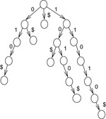
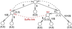
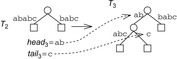
The algorithm takes a linear number of steps. If the extended locus of head_{i + 1} in T_i is found, the extension of the tree can be accomplished in constant time. Algorithm 3.42 has two stages. First, it determines head_{i + 1} in T_i in amortized constant time. Then, it sets another suffix link.

We observe that if

for character a and a (possibly empty) string γ, then γ is a prefix of head_{i + 1}. Let

, then there is a

, such that

is prefix of suf_i and suf_j according to the definition of head_i. Hence, γ is a prefix of suf_{i + 1} and suf_{j + 1}.

The loop invariants of the algorithm are (1) all internal nodes in T_{i − 1} have a correct suffix link in T_i (I1), and (2) during the construction of T_i the contracted locus of head_i in T_{i − 1} is visited (I2). The invariants are certainly true if

. If

, then (I2) implies that construction T_{i + 1} from T_i can start at the contracted locus of head_i in T_{i − 1}. If

, then let α_i be the concatenation of the edge labels of the path to the contracted locus of head_i without the first letter a_i. Moreover, β_i = head_i − a_i α_i; that is, head_i = a_i α_i β_i. If

, then T_i can be visualized as shown in Figure 3.28.

B9780123725127000031/f03-28-9780123725127.jpg is missing

Figure 3.28

Partition of T_i.

B9780123725127000031/u03-42-9780123725127.jpg is missing

Algorithm 3.42.

Algorithm to construct a Suffix Tree in linear time.

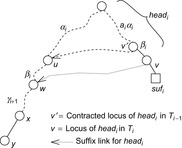
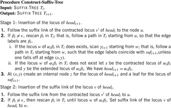
Based on the lemma we have

. From the contracted locus v′ of head_i we already have a correct suffix link in T_i to a node u according to (I1). To build the locus of head_{i + 1} in T_i we start at u instead of the root of T_i in the naive approach. In an actual implementation both stages would have to be interleaved.

Lemma 3.1

If the locus of

in T_i does not exist, then

Proof

Let v be the contracted locus and w be the extended locus of

. Let the labeling of the edges on the path to v be equal to γ and let the label of

be equal

with

and

. Then all suffixes with prefix

are contained in the subtree of T with root node w, and all suffixes in T have a prefix

. Therefore,

and suf_j has the prefix

. Hence, suf_j has the prefix

. We have to show that

and

with

Let suf_j′ be a suffix with prefix

. Then suf_{j′ + 1} has prefix

and suf_j′ has prefix

. Since

, the first letter a of δ₂ and the first letter b that follows

in suf_i are different. Therefore, the prefix of suf_{i + 1} is

and the prefix of suf_j is

, so that the longest common prefix is

As an example take

. The construction of T₁₄ from T₁₃ by inserting

in T₁₃ is shown in Figure 3.29.

B9780123725127000031/f03-29-9780123725127.jpg is missing

Figure 3.29

Construction of T₁₄ from T₁₃.

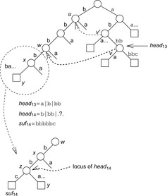
Theorem 3.7

(Time Complexity Suffix Tree Construction) Algorithm 3.42takes

time to generate a Suffix Tree for m.

Proof

In every step a suffix of m is scanned and rescanned. We first analyze rescanning. Since α_i β_i is a prefix of head_{i + 1}, at an edge we only have to test how many characters we have to skip in β_i. Subsequently, we require constant time for each traversed edge so that the total number of steps during rescanning is proportional to the number of traversed edges. Let

. At each edge e, which is traversed while rescanning β_{i − 1}, the string β_i is extended by δ of edge e; that is, δ is in res_i, but not in res_{i + 1}. Since

, we have

with k_i as the number of rescanned edges in step i, and

Next we analyze scanning. The number of scanned characters in step i equals

, where

Therefore, the total number of scanned characters is equal to

3.4.2. Generalized Suffix Trees

A Generalized Suffix Tree is a string data structure appropriate for web search and for solving problems in computational biology. After introducing Generalized Suffix Trees we first consider the problem of updating the information to obtain optimal space performance even in a dynamic setting.

The efficient construction of a Suffix Tree can be extended naturally to more than one string by building the Suffix Tree of the string

. It is not difficult to show (see Exercises) that the Suffix Tree for

is isomorphic to the compacted Trie for all suffixes of

up to all suffixes of

. Furthermore, the trees are identical except for the labels of the edges incident to leaves. This fact allows us to insert and search a string into an existing Suffix Tree.

A straightforward deletion of strings causes problems, since each edge stored at the subsequent nodes includes substring interval information of some previously inserted strings. Therefore, the update procedure also has to update substring references in the tree. The solution to this nontrivial problem is based on maintaining an additional Inverted Trie. Let M be the set of strings in the generalized Suffix Tree S and let T be the Trie that contains all inverted strings. Then there is a bijection between the set of nodes in T and the set of leaf nodes in S: On one hand, each suffix of a string m_i corresponds to a leaf node; on the other hand, for each prefix of

there is a prefix in T. Figure 3.30 shows a snapshot of inserting string 11010$ in a Generalized Suffix Tree with an associated inverted trie. Nodes of the same index indicate the bijection.

B9780123725127000031/f03-30-9780123725127.jpg is missing

Figure 3.30

Generalized Suffix Tree during insertion of 11010$.

Given the associated Inverted Trie, it is possible to delete a string from the largest suffix to the shortest. As a consequence, in each step the suffix links are correct. The problem that is often not dealt with in literature is that the deleted strings are indeed needed inside the generalized tree. The idea of the improvement is to extend the unique representation of the leaves given by T bottom to the internal nodes. Therefore, we invent twins that refer to the history of leaf generation. Figure 3.31 gives an example.

B9780123725127000031/f03-31-9780123725127.jpg is missing

Figure 3.31

Twin structure in the Generalized Suffix Tree.

As with the algorithm for constructing an ordinary Suffix Tree, the insertion process can be divided into a sequence of update operations. In the pseudo-code implementation of Algorithm 3.43 we assume a procedure to insert a suffix at an existing locus, and a procedure to split an existing edge. Deletion, as shown in Algorithm 3.44, is based on a subroutine for removing a leaf that is called for each removed node while deleting the inverted string in the Inverted Trie T. If removing a leaf, we access and adjust the string representation of a twin. The correctness argument is based on the following result.

B9780123725127000031/u03-43-9780123725127.jpg is missing

Algorithm 3.43.

Insertion of one suffix in a Generalized Suffix Tree.

B9780123725127000031/u03-44-9780123725127.jpg is missing

Algorithm 3.44.

Deleting a string in a Generalized Suffix Tree.

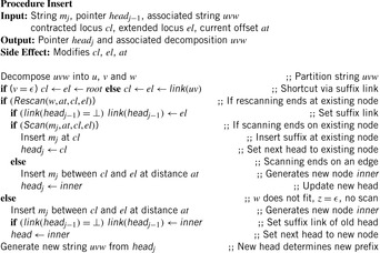
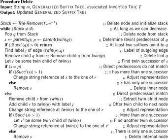
Lemmma 3.2

Let Internal and Leaves be the sets of all internal and leaf nodes in the Generalized Suffix Tree. Let

be the set of successor of p and

be the set of twin successors of p. The following invariances are preserved:

(Ia) For all

there is a

with

, which has the same string representative as p.

(Ib) For all

we have

; that is, the number of ordinary successors is always one larger to the number of twin successors.

Proof

To prove the result we perform a case study:

Inserting a suffix at a given node A newly inserted leaf extends both sets

and

for the existing node by one element. The string representation of the leaf and of the existing node is set to the inserted string m. Therefore, the invariances remain satisfied.

Inserting a suffix between two nodes In this case both newly generated nodes refer to m, so that we have (Ia). The internal node gets two successors and one twin successor (the new leaf node). Therefore,

and (Ib).

Removing a Leaf Let q be the node to be deleted, s be its predecessor, and p its twin predecessor. The algorithm considers two cases:

[

] Since q in

invariance (Ib) is satisfied. If

, then there exists a leaf r in

. Leaf r changes the string representation such that s no longer refers to the string representation of q. Therefore, we have (Ia) for node s. If, however,

, then s is deleted for good, and nothing has to be shown.

[

] This case is tricky. If

, then s is deleted. Moreover,

is set to

such that

remains unchanged. Otherwise,

. Using (Ib), then at the time when q was deleted we have

successors and k twin successors of s. Consequently, besides

there is another twin successor r of s. This node is used to determine the string representation for p; that is,

is set to

. We see that both invariances are maintained.

Hence, we can prove the following result.

Theorem 3.8

(Space Optimality Generalized Suffix Tree) Let S be a Generalized Suffix Tree after an arbitrary number of insert and delete operations and

be the maximal number of all characters of strings in the dictionary M; that is,

, where i denotes the operation step. The space requirements of S are bounded by

To find a substring of a given string m, we can determine the longest pattern prefix h of the string stored in the Generalized Suffix Tree that matches m starting at position i,

. Similarly, we can determine the longest substring h of the strings stored in the Generalized Suffix Tree that matches m ending at position i. In both cases we have to check if h is maximal; that is, if an accepting node that corresponds to a path for a full string m in the dictionary has been reached.

3.5. Summary

The search algorithms discussed in the previous chapter need to keep track of the generated and expanded states. A*, for example, needs to be able to check whether a state is in the Open list, insert a state into the Open list, with a given f-value, decrease the f-value of a state in the Open list, extract the state with the smallest f-value from the Open list, check whether a state is in the Closed list, insert a state into the Closed list, and perhaps delete a state from the Closed list. These operations need to be fast since they are typically performed a large number of times during each search. In this chapter, therefore, we discussed algorithms and data structures for implementing them.

The Open list is basically a priority queue. The values of the priorities (e.g., the f-values for A*) determine how the operations on the Open list can be implemented. If the priorities are floating-point values, then the operations can be implemented with heaps, including advanced heap structures and data structures. A Heap is a complete binary tree that stores a state at every node so that the priority of the state at a node is always higher than the priority of the states at the children of the node. A Fibonacci Heap, a Weak Heap, and a Weak Queue relax this requirement in different ways. If the priorities are integers, then the operations can also be implemented with buckets of fixed or exponentially increasing sizes (Radix Heap) or hierarchical structures of buckets, including the Van Emde Boas Priority Queue. Buckets consist of randomly accessible storage locations in a consecutive address range that are labeled with consecutive ranges of priorities, where each storage location stores the set of states of which the priorities are in its range of priorities. Implementations that use buckets are usually faster than those that use heaps.

Table 3.4 gives an overview for the priority queue data structures introduced in this chapter. The complexities for integer-based methods are measured in the number of instructions. For generic weights we express complexities in the number of comparisons. The parameters are C= max edge weight, N= max key, n= nodes stored, and e= nodes visited. The star (*) denotes amortized costs.

**Table 3.4** Priority queue data structures; top are bucket structures for integer keys, bottom are heap structures for general keys in a totally ordered set defined through a comparison function.
Data Structure	DecreaseKey	DeleteMin	Insert	Dijkstra/A*
1-Level Bucket (Algorithm 3.1, Algorithm 3.2, Algorithm 3.3 and Algorithm 3.4)	O (1)	O (C)	O (1)	O (e + Cn)
2-Level Bucket	O (1)		O (1)
Radix Heap (Algorithm 3.5, Algorithm 3.6, Algorithm 3.7 and Algorithm 3.8)	O (1)*	O (lg C)*	O (1)*	O (e + n ⋅ lg C)
Emde Boas (Algorithm 3.9, Algorithm 3.10 and Algorithm 3.11)	O (lg lg N)	O (lg lg N)	O (lg lg N)	O ((e + n) lg lg N)
Binary Search Tree	O (lg n)	O (lg n)	O (lg n)	O ((e + n) lg n)
Binomial Queue	O (lg n)	O (lg n)	O (lg n)	O ((e + n) lg n)
Heap (Algorithm 3.12, Algorithm 3.13 and Algorithm 3.14)	2lgn	2lgn	2lgn	O ((e + n) lg n)
Weak Heap (Algorithm 3.17, Algorithm 3.18, Algorithm 3.19, Algorithm 3.20 and Algorithm 3.21)	lgn	lgn	lgn	O ((e + n) lg n)
Pairing Heap (3.16)		O (lg n)*	O (1)
Fibonacci Heap (3.22)	O (1)*	O (lg n)*	O (1)	O (e + nlgn)
Rel. Weak Queue (3.23)	O (1)	O (lg n)	O (1)	O (e + nlgn)

The Closed list is a simple set. The operations on it can, therefore, be implemented with bitvectors, lists, search trees, or hash tables. Bitvectors assign a bit to every state in a set. The bit is set to one if the state is in the set. They are a good choice if the percentage of states in the set (out of all states) is large. Lists simply represent all states in the set, perhaps storing compressed versions of states by representing similar parts of several states only once (Suffix Tree list). They are a good choice if the percentage of states in the set is small. The question then becomes how to test membership efficiently. To this end, lists are often represented as search trees or, more commonly since faster, hash tables rather than linked lists. Hash tables (hash dictionaries) consist of randomly accessible storage locations in a consecutive address range. Hashing maps each state to an address.

We discussed different hash functions. Perfect hashing (similar to bitvectors) maps every state to its own address. To insert a state into a hash table, we store the state at its address. To delete a state from the hash table, we remove the state from its address. To check whether a state is in the hash table, we compare the state in question against the state stored at its address. If and only if there is a state stored at its address and it matches the state in question, then the state in question is in the hash table. Perfect hashing is memory intensive. Regular hashing can map two states to the same address, which is called an address collision. Address collisions can be handled either via chaining or open addressing. Chaining resolves the conflict by storing all states in the hash table that map to the same address in a linked list and stores a pointer to the linked list at this address. Open addressing resolves the conflict by storing a state at a different address in either the same or a different hash table when some other state is already stored at its address. We discussed different ways of determining this other address, including using more than one hash table.

We also discussed how to increase the size of the hash table, in case the number of successive address collisions is too large, until an empty address is found. Regular hashing is less memory intensive than perfect hashing but can still be memory intensive. Approximate hashing saves memory by storing an insufficient amount of information to implement the membership test exactly. For example, it might store only a compressed version of the state in one or more hash tables. In the extreme case, it might only set a single bit to one in one or more hash tables to indicate that some state is stored at an address. In case of several hash tables, the state is considered stored if and only if all hash tables report that it is stored. Approximate hashing can make the mistake to determine that a state is in the Closed list even though it is not, which means that a search might not expand a state since it thinks it has expanded the state already and thus might not be able to find a path even if one exists.

Table 3.5 gives an overview of the different hash methods and their time complexity. We indicate whether states are stored in a compressed or ordinary way, and whether or not the hashing method is lossy.

**Table 3.5** Hashing algorithms. With Y we denote . With p⁺ (α) and p⁻(α) we denote the time complexities for successful and unsuccessful search based on the current hash table load α. More accurate values depend on the conflict resolution strategy used.
	Insert	Lookup	Compressed	Lossy
Chaining (Algorithm 3.29, Algorithm 3.30 and Algorithm 3.31)	O (1)	O (Y)	–	–
Open addressing (Algorithm 3.32, Algorithm 3.33, Algorithm 3.34 and Algorithm 3.35)	O (p⁻(α))	O (p⁺ (α))	–	–
Suffix List hashing	O (lgn)*	O (lgn)*	√	–
FKS hashing	O (1)*	O (1)	–	–
Cuckoo hashing (Algorithm 3.36, Algorithm 3.37 and Algorithm 3.38)	O (1)*	O (1)	–	–
Bit-state hashing	O (1)	O (1)	√	√
Hash compact	O (1)	O (1)	√	√

Moreover, we have seen two storage structures for partial information. The subset dictionary stores partial states in the form of sets, and the substring dictionary stores partial paths in the form of substrings. In the first case, different implementations have been discussed to solve one of the equivalent problems, Subset Query, Containment Query, and Partial Match; for the second case, we have concentrated on the Suffix Tree data structure and its extensions for solving the Dynamic Dictionary Matching problem.

3.6. Exercises

3.1 Display the

1. 2-Level Bucket data structure (C = 80)

2. Radix Heap data structure

for the elements {28, 7, 69, 3, 24, 7, 72}.

3.2 A union-find data structure is a dictionary for maintaining partitions of a set. We may represent each interval by its right-most element, so that the partitioning

is represented by the set

. Consider the data type that represents a partition of

into intervals with the operations:

• Find (x) that returns the interval containing x.

• Union (x) that unifies an interval with the immediately following one.

• Split (x) that splits the interval T containing x into two intervals

and

1. How do the basic operations act on this set?

2. Use a Van Emde Boas Priority Queue to implement this strategy.

3.3 In a randomly filled array with n entries the minimal and maximal elements have to be found. For the sake of simplicity, you may assume

to be a power of 2.

1. Describe a divide-and-conquer algorithm that uses

comparisons.

2. Use Weak Heaps to elegantly solve the problem with

comparisons.

3. Show as a lower bound

comparisons are required to solve the problem.

4. Show a similar bound to search the first- and second-smallest element.

3.4

1. Show that the path to index n in a Heap is determined by the binary representation of n.

2. Let f (n) be the number of Heaps with n pairwise different keys and let s_i be the size of the subtree for root i,

. Show that

3.5 Merge two Heaps with n₁ and n₂ elements efficiently.

1. Assume that n₁ und n₂ are very different; for example, n₁ is much larger than n₂.

2. Assume that n₁ and n₂ are almost the same, say

Provide the time complexities for both cases in big-oh notation.

3.6 Double-ended queues are priority queues that allow the insertion and the deletion of the minimum and maximum element.

1. Transform a Heap/Weak Heap into its dual and estimate the number of required comparisons.

2. Show how to perform the transposition of elements in such a compare-exchange structure.

3.7 Transform a Weak Heap into a heap in-place with a small number of comparisons.

1. Study the base case of a Weak Heap of size 8.

2. Develop a recursive algorithm. For the ease of construction, you may assume

3. Compare the number of comparisons with ordinary heap construction and top-down, bottom-up, and binary search sift-down.

3.8 In an initially empty Binomial Queue perform the following operations:

1. Insert(45), Insert(33), Insert(28), Insert(21), Insert(17),Insert(14)

2. Insert(9), Insert(6), Insert(5), Insert(1),DeleteMin

3. DecreaseKey(33,11), Delete(21), DecreaseKey(28,3),DeleteMin

Display the data structure for all intermediate results.

3.9 Consider an initially empty hash table with 11 entries. Insert the keys 16, 21, 15, 10, 5, 19, and 8 according to the following hash algorithms and display the table after the last insertion. Use the two hash functions

and

1. Linear probing using

, quadratic probing using

2. Double and ordered hashing, single and double bit-state hashing.

3.10 Let

be a state for an Atomix problem on a board of size

. We define its hash value as

. Let v be an immediate successor of u that differs from its predecessor u only in the position of atom i.

1. Determine h (v) based on h (u) using incremental hashing.

2. Use a precomputed table with

entries to accelerate the computation.

3. Avoid computationally expensive modulo operators by using addition/subtraction.

3.11 Dynamic incremental hashing considers hashing of state vectors of variable size.

1. How does the hash function

change if:

• A value is added to/deleted at the end of the existing state vector of u?

• A value is added to/deleted at the beginning of the existing state vector of u?

For both cases devise a formula that can be computed in time O (1).

2. For the general case, where a value is changed somewhere in the state vector

, compute the hash address in

time.

3.12 In the Suffix Tree list example of Figure 3.18, insert

and delete

3.13 Compute the

1. perfect hash value of the permutation

2. permutation (of size 15) for the rank

according to the lexicographic ordering and according to the one of Myrvold and Ruskey.

3.14 Devise two hash functions and a sequence of insertions that lead to an infinite cuckoo process.

3.15 Let

. A Navigation Pile is a complete binary tree with

nodes. The first

leaf elements store one element each and the remaining leaves are empty. Interior nodes (branches) contain links to the leaf nodes in the form of binary-encoded relative index information. For each branch the leaf is addressed that contains the smallest element of all elements stored in the leaf sequence.

The representation of a Navigation Pile are two sequences:

for the elements and

for the navigation information, pointing to the elements in A. An example Navigation Pile of size 14 and capacity 16 are shown in Figure 3.32. The parent/ child relationship is shown with dotted arrows and the navigation information with solid arrows.

B9780123725127000031/f03-32-9780123725127.jpg is missing

Figure 3.32

Example of a Navigation Pile.

1. Show that all navigation information can be stored with

bits.

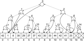
2. Argue that the following operations can be supported in constant time: depth, height, parent, first-leaf, last-leaf, first-child, second-child, root, is-root, and ancestor.

3. Show that bottom-up construction of a Navigation Pile requires

comparisons.

4. Show how to implement Insert with at most

comparisons and one element move (given that

additional instructions are allowed).

3.16 Draw a Suffix Tree for 10100100110001100$ including the suffix links.

3.17 Consider a text t.

1. Show how to report all substrings in t in between two given strings with respect to their lexicographic ordering. For example, ACCGTA is in between ACA and ACCT.

2. Devise an efficient algorithm to find the longest substring that occurs at least twice in t.

3.18 There are

substrings of string T of size n. Some of the substrings are identical.

1. Show that

has

different substrings.

2. Show how to print all different substrings in time proportional to their total length.

3.19 Let D be a set of k string of length

1. Devise an efficient algorithm to determine for each string in D if it is a substring of another string in D.

2. Devise an algorithm that computes the longest common substring for all pairs of strings in D. The running time should be

, where d is the sum of the sizes of the strings in D.

3. Let

. Devise an algorithm that computes the longest common prefix for all pairs of strings in D. The running time should be

, where p is the number of pairs, of which the common prefix is not empty.

3.20 Consider a (very long) text T = t₁…t_n over the alphabet Σ to be searched for a maximal pattern P = t_it_{i + 1}…t_j such that the reflection

is also a pattern in T. For example, in T = 10000111100101111000001 the pair P = 000011110 and

is maximal. Describe an efficient algorithm to solve the problem and provide its time and space complexities.

3.7. Bibliographic Notes

Dial (1969) has invented the 1-Level Bucket priority queue data structure. Its variants have been studied by Ahuja, Magnanti, and Orlin (1989). The 2-level architecture can be further refined to an arbitrary number k of levels, with k-arrays of the size

. Space and time can be improved to

, but the implementation becomes quite involved. Two-layered Radix Heap data structures improve the bound for DeleteMin to

and a hybrid with a Fibonacci Heap yields an

time algorithm. Alternative priority queue data structures based on keys have been studied by van Emde Boas, Kaas, and Zijlstra (1977). Dementiev, Kettner, Mehnert, and Sanders (2004) have provided cache-efficient implementations.

Fredman and Tarjan (1987) have given the amortized analysis for a Fibonacci Heap that apply Insert and DecreaseKey in amortized constant time and DeleteMin in amortized logarithmic time. Cherkassy, Goldberg, and Silverstein (1997b) compare different priority queue implementations and provide an efficient shortest path library (Cherkassy, Goldberg, and Ratzig, 1997a). Many priority queue implementations have been integrated in LEDA by Mehlhorn and Näher (1999).

The Weak Heap data structure has been introduced by Dutton (1993) and analyzed in detail by Edelkamp and Wegener (2000). Edelkamp and Stiegeler (2002) have implemented a sorting index based on Weak Heapsort with

comparisons in the worst-case and an in-place Quicksort variant with

comparisons on average. The latter approach is based on replacing original Heapsort with Weak Heapsort in the hybrid of Quick-Heapsort originally proposed by Cantone and Cinotti (2002).

Minimizing the number of moves has been considered by Munro and Raman (1996). The Navigation Pile data structure has been introduced by Katajainen and Vitale (2003). It has been applied to sorting, yielding an algorithm with

comparisons,

element moves, and

further instructions. Independently, Franceschini and Geffert (2003) devised a sorting algorithm with less than

moves and

comparisons. Other doubly ended priority queue structures are min-max Heaps proposed by Atkinson, Sack, Santoro, and Strothotte (1986), Deaps by Carlsson (1987) and Interval Heaps by van Leeuwen and Wood (1993).

Thorup (1999) has shown that for integer weights in undirected graphs a deterministic linear-time algorithm can be devised. It bypasses the requirement for extracting the minimum element. The data structure is substituted by a growing Component Tree. However, the algorithm is pretty involved and rather of theoretical interest, since its data structure, an Atomic Heap, requires

. Thorup (2000) has studied RAM priority queues. For a random access machine with arbitrary word size a priority queue is obtained supporting Insert, Delete, and DeleteMin operations in worst-case time

. This improves

for a hybrid Radix Heap. Relaxed Weak Queues (a.k.a. Run-Relaxed Weak Queues) by Elmasry, Jensen, and Katajainen (2005) are binary tree variants of run-relaxed heaps invented by Driscoll, Gabow, Shrairman, and Tarjan (1988) and implement a worst-case efficient priority queue (with constant-time efficiencies for Insert and DecreaseKey and logarithmic time for Delete and DeleteMin). Other structures achieving this performance are Brodal Heaps by Brodal (1996) and Fat Heaps by Kaplan, Shafrir, and Tarjan (2002). By sacrificing worst for average case performance, Rank-Relaxed Weak Queues achieve a better practical efficiency. Another promising competitor in this class are Violation Heaps proposed by Elmasry (2010). Policy-based benchmarking has been done by Bruun, Edelkamp, Katajainen, and Rasmussen (2010).

Theoretical advances for reducing the number of comparisons for deleting the minimum to

and

have been discussed by Elmasry, Jensen, and Katajainen (2008c) and Elmasry, Jensen, and Katajainen (2008b). Pairing Heaps have been suggested by Fredman, Sedgewick, Sleator, and Tarjan (1986). A refined implementation has been suggested by Stasko and Vitter (1987). A transformational approach and survey on efficient double-ended priority queues has been provided by Elmasry, Jensen, and Katajainen (2008a).

Hashing is fundamental to state space search and by the need of good distribution functions links to the generation of pseudo-random numbers. One generator has been proposed by Lehmer (1949) and its improvement has been suggested by Schrage (1979). The distribution and the selection of good random numbers have been analyzed by Park and Miller (1988).

Karp and Rabin (1987) have suggested incremental hashing for string search. A related incremental hashing for game playing has been introduced by Zobrist (1970). Its application to state space search and multiple pattern databases has been proposed by Mehler and Edelkamp (2005). For dynamic state vectors, incremental hashing has been extended by Mehler and Edelkamp (2006). Recursive hashing has been introduced by (Cohen 1997) and most prominently implemented in the software model checker SPIN (Holzmann 2004). Gains for incremental recursive hashing in SPIN are documented by Nguyen and Ruys (2008). In this context universal hashing has been shown to have advantages by Eckerle and Lais (1998). In experiments the authors have shown that the ideal circumstances for error prediction in sequential hashing are not found in practice and refine the model for coverage prediction to match the observation. Bit-state hashing has been adopted in protocol validator SPIN that parses the expressive concurrent Promela protocol specification language (Holzmann, 1998). Hash compaction has been contributed by Stern and Dill (1996) and collapse compression has been implemented by Holzmann (1997) and Lerda and Visser (2001).

The Bloom Filter has been invented by Bloom (1970) and been used in the web context by Marais and Bharat (1997) as a mechanism for identifying which pages have associated comments stored. Holzmann and Puri (1999) have suggested a finite-state machine description that shares similarities with binary decision diagrams. In work by Geldenhuys and Valmari (2003) the practical performance ratio has been shown to be close to the information theoretical bound for some protocols like the Dining Philosophers. As with the suffix list by Edelkamp and Meyer (2001) the construction aims at redundancies in the state vector. Similar ideas have been considered by Choueka, Fraenkel, Klein, and Segal (1986), but the data structure there is static and not theoretically analyzed. Another dynamic variant achieving asymptotically equivalent storage bounds is sketched in Brodnik and Munro (1999). Constants are only given for two static examples. Comparing with the numbers of Brodnik, a dynamic Suffix Tree list can host up to five times more elements of the same value range. However, the data structure of Brodnik provides constant access time.

Ranking permutations in linear time is due to Myrvold and Ruskey (2001). Korf and Schultze (2005) have used lookup tables with a space requirement of

bits to compute lexicographic ranks, and Bonet (2008) has discussed different time-space trade-offs. Mares and Straka (2007)proposed a linear-time algorithm for lexicographic rank, which relies on constant-time bitvector manipulations.

FKS hashing is due to Fredman, Komlós, and Szemeródi (1984). Dietzfelbinger, Karlin, Mehlhorn, auf der Heide, Rohnert, and Tarjan (1994) have devised the first dynamic version of it, yielding a worst-case constant-time hashing algorithm. Östlin and Pagh (2003) have shown that the space complexity for dynamical perfect hashing can be greatly reduced and Fotakis, Pagh, and Sanders (2003) have studied how to further reduce the space complexity to an information theoretical minimum. Practical perfect hashing has been analyzed by Botelho, Pagh, and Ziviani (2007) and an external memory perfect hash function variant has been given by Botelho and Ziviani (2007). The complexity is bounded by the need to sort all elements by their hash value in the partitioning step. Minimum perfect hash functions can be stored with less than four bits per item. With cuckoo hashing, Pagh and Rodler (2001) have devised a further practical and theoretical worst-case optimal hashing algorithm.

The Suffix Tree data structure is of widespread use in the context of web search (Stephen 1994) and computational biology (Gusfield 1997). The linear-time construction algorithm is due to McCreight (1976). Dynamic Dictionary Matching problems have been proposed and solved by Amir, Farach, Galil, Giancarlo, and Park (1994) and Amir, Farach, Idury, Poutré, and Schäffer (1995). The optimal space bound for arbitrary deletions has been proven by (Edelkamp 1998b). Another class for string search based on bit manipulation has been contributed by Baeza-Yates and Gonnet (1992).

Probably the first nontrivial result for the Partial Match problem has been obtained by Rivest (1976). He showed that the 2^m space of the exhaustive storage solution can be improved for

. New algorithms for subset queries and partial matching have been provided by Charikar, Indyk, and Panigrahy (2002), studying two algorithms with different trade-offs. The Rete algorithm is due to Forgy (1982). The related Two-Dimensional Pattern String Matching problem has been studied intensively in literature, for example, by Fredriksson, Navarro, and Ukkonen (2005). Hoffmann and Koehler (1999) have suggested Unlimited Branching Trees.

..................Content has been hidden....................

You can't read the all page of ebook, please click here login for view all page.

Table of Contents for Chapter 3. *Dictionary Data Structures

Create new playlist

Sign In

Sign Up

3.1. Priority Queues

3.1.1. Bucket Data Structures

Buckets

Multilayered Buckets

Radix Heaps

Van Emde Boas Priority Queues

3.1.2. Heap Data Structures

Binary Search Trees

Heaps

Pairing Heaps

Weak Heaps

Fibonacci Heaps

Relaxed Weak Queues

3.2. Hash Tables

3.2.1. Hash Dictionaries

3.2.2. Hash Functions

Remainder Method

Multiplicative Hashing

Rabin and Karp Hashing

Incremental Hashing

Universal Hash Functions

Perfect Hash Functions

Lexicographic Ordering

Myrvold Ruskey Ordering

3.2.3. Hashing Algorithms

FKS Hashing Scheme

Dynamic Perfect Hashing

Cuckoo Hashing

3.2.4. Memory-Saving Dictionaries

Suffix Lists

3.2.5. Approximate Dictionaries

Bit-State Hashing

Hash Compaction

Collapse Compression

3.3. Subset Dictionaries

3.3.1. Arrays and Lists

3.3.2. Tries

3.3.3. Hashing

3.3.4. Unlimited Branching Trees

3.4. String Dictionaries

3.4.1. Suffix Trees

3.4.2. Generalized Suffix Trees

3.5. Summary

3.6. Exercises

3.7. Bibliographic Notes

Table of Contents for
Chapter 3. *Dictionary Data Structures