
Chapter 12. Adversary Search
This chapter studies heuristic search in game graphs. For two-player games, tree search from the current node is performed and endgame databases are built. The chapter discusses different refinement strategies to improve the exploration for forward search and suggests a symbolic classification algorithm.
Keywords: two-player game, game tree search, AND/OR graph, minimax search, negmax search, alpha-beta pruning, null window search, principle variation search, memory-enhanced test driver, partition search, best-first game tree search, conspiracy search, UCT, retrograde analysis, multiplayer game, general game playing, AO* search, LAO* search
Adversaries introduce an element of uncertainty into the search process. One model for adversary search is game playing. It is a special case of a layered tree search that has been investigated in depth using specialized algorithms. Optimal strategies result in perfect play. In most settings, the players can take actions alternately and independently. We address the standard game playing algorithms negmax and minimax together with pruning options like αβ. Game tree searches are rather depth-bounded rather than cost-bounded, and values at the leaf nodes of the tree are computed through a static evaluation function. Retrograde analysis calculates entire databases of classified positions in a backward direction, starting from won and lost ones; these databases can be used in conjunction with specialized game playing programs as endgame lookup tables. Multiplayer and general game playing broaden this scope.
In nondeterministic or probabilistic environments, the adversary refers to the unpredictable behavior of nature. In contrast to the deterministic search models, the outcome of an executed action in a state is not unique. Each applicable action may spawn several successors. There are many reasons for such uncertainty: randomness that is in the real world, the lack of knowledge for modeling the real world precisely, the dynamic change in the environment that we cannot control, sensors and actuators that are imprecise, and so on.
Solutions to nondeterministic and probabilistic search tasks are no longer sequences of actions but mappings from state to actions. As opposed to linear solution sequences, adversary search requires state space traversal to return solution policies in the form of a tree or a graph. The policy is often implicitly represented in the form of a value function that assigns a value to each of the states. For the deterministic setting, the value function takes the role of the heuristic that is gradually improved to the goal distance. This links the solution process for adversary search problems to the ones presented for real-time search, where the value function for deterministic search models is improved over time.
To apply policies to the real world, we embed the solutions in the environment in the form of finite-state controllers. This means that solutions can be interpreted as being programs that react on inputs by issuing an action in the current internal state and changing this state based on the response of the environment.
In a probabilistic environment the standard formalism for a stochastic search problem is that of a Markov decision process. A simpler model of nondeterminism is an AND/OR graph, in which the solver controls the OR nodes, and the environment operates on the AND nodes. The main difference between the two is that outgoing edges when performing actions are labeled with probabilities.
We unify solving deterministic, nondeterministic, and probabilistic searches in one model. As with deterministic search, we usually search for policies that are optimal. In nondeterministic and probabilistic environments, the intended effect might be achieved or not; in this case, we maximize the expected rewards (or minimize the expected costs ).
12.1. Two-Player Games
According to John McCarthy, Chess is the Drosophila of AI, in an analogy with dominant use of that fruit fly to study inheritance. Since the early 1950s, Chess (see Fig. 12.1) has advanced to one of the main successes in AI, resulting in the defeat of the human world champion in a tournament match, even if we may argue on how the computation-intense search resemblances to the intellectual approach used by human players.
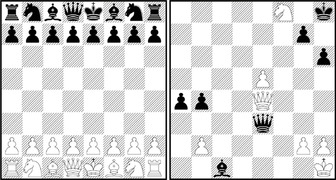
Generally, a move in Chess consists of transporting one of the pieces of the player to a different square, following the rules of movement for that piece. Up to one exception, a player can take a piece of the opponent by moving one of his own pieces to the square occupied by the opponent. The opponent's piece is removed from the board and remains out of play for the rest of the game. When the king is threatened and cannot make a move such that after the move the king is not threatened, then we have a mate position, which ends the game (see Fig. 12.1, right, for a mate in one move). When a player cannot make any legal move, but the king is not threatened, then the game is a draw. If the same position with the same player to move is repeated three times, he can also claim a draw.
The position to the right in Figure 12.1 illustrates a move in a recent human-machine game that has been overseen by the human world champion when playing against the program Deep Fritz. The personal computer won by 4:2. In contrast, Deep Thought, the first computer system that defeated a human world champion in a match, used a massively parallelized, hardware-oriented search scheme, evaluating and storing billions of nodes in a second with a fine-tuned evaluation function and a large, human-made opening book.
Besides competitive play, some combinatorial Chess problems, like the 33,439,123,484,294 complete Knight's tours, have been solved using search.
Tic-Tac-Toe (see Fig. 12.2) is a game between two players, who alternate in setting their respective tokens O and X on a 3 × 3 board. The winner of the game has to complete either a row, a column, or a diagonal with his own tokens. Obviously, the size of the state space is bounded by 39 = 19,683 states, since each field is either unmarked, or marked X or O. A complete enumeration shows that there is no winning strategy (for either side); the game is a draw (assuming optimal play).
Nim is a two-player game in which players remove one or more matches at a time from a single row. The player to take the last match wins. One classic Nim instance is shown in Figure 12.2 (right). By applying combinatorial game theory an optimal playing strategy can be obtained without much search (see Exercises).
Strong Go programs try to emphasize much of the human way of thinking rather than brute-force search methods for which computers are ideal, and from this point of view Go might have a chance to become the next fruit fly of AI, in the sense of McCarthy. Many techniques, like rule-based knowledge representation, pattern recognition, and machine learning, have been tried. The two players compete in acquiring territory by placing stones on a 19 × 19 board (see Fig. 12.3, left). Each player seeks to enclose territory with his stones and can capture opponent's ones. The object of the game is to enclose the largest territory. The game has been addressed by different strategies. One approach with exponential savings in some endgames uses a divide-and-conquer method in which some board situations are split into a sum of local games of tractable size. Another influencing search method exploits structure in samples of random play.
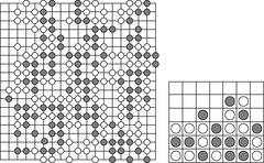
In Connect 4 (see Fig. 12.3, right), a player has to place tokens into one of the lowest unoccupied fields in each column. To win, four tokens of his color have to be lined up horizontally, vertically, or diagonally before the opponent does. This game has been proven to be a win for the first player in optimal play using a knowledge-based minimax-based search that introduces the third value unknown into the game search tree evaluation. The approach has a working memory requirement linear in the size of the search tree, whereas traditional αβ pruning requires only memory linear to the depth of it.
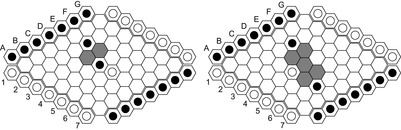
The basic aim of the board game Nine-Men-Morris (see Fig. 12.4) is to establish vertical or horizontal lines (a mill). Whenever a player completes a mill, that player immediately removes one opponent piece that does not form part of a mill from the board. If all the opponent's pieces form mills then an exception is made and the player is allowed to remove one. Initially, the players place a piece of their own color on any unoccupied point until all 18 pieces have been played. After that, play continues alternately but each turn consists of a player moving one piece along a line to an adjacent point. The game is lost for a player either by being reduced to two pieces or by being unable to move. Nine-Men-Morris has been solved with parallel search and huge endgame databases. The outcome of a complete search is that the game is a draw.
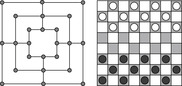
In Checkers (see Fig. 12.4, right) the two players try to capture all the other players' pieces or render them immobile. A regular piece can move to a vacant square, diagonally forward. When such a regular piece reaches the last row, it becomes a king. A king can move to a vacant square diagonally forward or backward. A piece (piece or king) can only move to a vacant square. A move can also consist of one or more jumps, capturing an opponent piece if jumped. Nowadays, checker programs have perfect information for all Checkers positions involving 10 or fewer pieces on the board generated in large retrograde analysis using a network of workstations and various high-end computers. Checkers is a draw.
Hex (see Fig. 12.5, left) is another PSPACE-complete board game. The players place balls in one of the cells with their color. Both players attempt to build a chain of his colored cells connecting his (opposing) borders. Since the game can never result in a draw, it is easy to prove that the game is won for the first player to move, since otherwise he can adopt the winning strategy of the second player to win the game. In Hex the current state-of-the-art programs use an unusual approach of electrical circuit theory to combine the influence of subpositions (virtual connections) to larger ones. A virtual semiconnection allows two groups of pieces to connect provided that one can move, and a full virtual connection allows groups to connect independent of the opponent's moves (see Fig. 12.6).
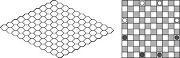
Amazons (see Fig. 12.5, right) is a board game, which has become popular in recent years, and has served as a platform for both game-theoretic study and AI games research. Players move queens on an n × n (usually 10 × 10) board. The pieces, called queens or amazons, move like Chess queens. As part of each move an arrow is shot from the moved piece. The point where the arrow lands is reachable from the target position and is eliminated from the playing area, such that the arrows eventually block the movement of the queens. The last player to complete a move wins. Amazons is in PSPACE, since (unlike Chess and Go) the number of moves in an Amazons game is polynomially bounded. Deciding the outcome of n × n Amazons is PSPACE-hard.
12.1.1. Game Tree Search
To select an optimal move in a two-person game, the computer constructs a game tree, in which each node represents a configuration (e.g., a board position). The root of the tree corresponds to the current position, and the children of a node represent configurations reachable in one move. Every other level (a.k.a. ply) corresponds to opponent moves. In terms of the formalism of Section 12.4, a game tree is a special case of an AND/OR graph, with alternating layers of AND and OR nodes. We are particularly concerned here with zero-sum games (the win of one player is the loss of the other), where both players have perfect information (unlike, for example, in a card game).
Usually, the tree is too large to be searched entirely, so the analysis is truncated at some fixed level and the resulting terminal nodes are evaluated by a heuristic procedure called a static evaluation function. The need for making a decision sooner than it takes to determine the optimal move and the bounded backup of horizon estimates is a characteristic that two-player search shares with real-time search.
The evaluation procedure assigns a numeric heuristic value to the position, where larger values represent positions more favorable to the player whose turn is to play. The static evaluator doesn't have to be correct, the only requirement is that it yields the correct values for terminal positions (e.g., checkmate or drawn configurations in Chess), and the informal expectation that higher values correlate with better positions, on average. There is no notion of admissibility as in single-player games. A static evaluator can be implemented using basically any appropriate representation. One common, simple form is a weighted sum of game-specific features, such as material difference, figure mobility, attacked figures, and so on.
A major share of the secret of writing strong computer games lies in the “black magic” of crafting good evaluation functions. The challenge lies in striking the right balance between giving an indicative value without excessive computational cost. Indeed, easy games can be searched completely, so almost any heuristic will do; on the other hand, if we had an evaluation function at hand that is always correct, we wouldn't have to search in the first place. Usually, evaluation functions are developed by experts in laborious, meticulous trial-and-error experimentation. However, we will later also discuss approaches to let the computer “learn” the evaluation on its own.
It is a real challenge to find good evaluation functions for interesting games that can be computed efficiently. Often the static evaluation function is computed in two separate steps. First, a number of features are extracted, then these features are combined to an overall evaluation function. The features are described by human experts. The evaluation function is also often derived by hand, but it can also be learned or optimized by a program. Another problem is that all feature values have to be looked at and that the evaluation can become complex. We give a solution based on classification trees, a natural extension of decision trees, which are introduced first. Then we show how classification trees can be used effectively in αβ-search and how to find the evaluation functions with bootstrapping.
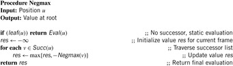
We will assume that the value of a position from the point of view of one player is the negative of its value from the point of view of the other. The principal variation is defined as the path from the root on which each player plays optimally; that is, chooses a move that maximizes his worst-case return (as measured by the static evaluator at the leaves of the tree). It may be found by labeling each interior node with the maximum of the negatives of the values of its children. Then the principal variation is defined as the path from the root to a leaf that follows from each node to its lowest-valued child; the value at the root is the value of the terminal position reached by this path (from the point of view of the first player). This labeling procedure is called the negmax algorithm, with its pseudo code shown in Algorithm 12.1.
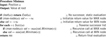
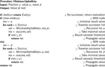
Minimax is an equivalent formulation of negmax, where the evaluation values for the two players do not necessarily have to be the negative of each other. The search tree consists of two different types of nodes: the MIN nodes for one player that tries to minimize the possible payoff, and the MAX nodes for the other player that tries to maximize it (see Alg. 12.2).
For all but some trivial games, the game tree cannot be fully evaluated. In practical applications, the number of levels that can be explored depends on a time limit for this move; in this respect, the interleaving of computation and action is reminiscent of the real-time search scenario (see Chapter 11). Since the actually required computation time is not known beforehand, most game playing programs apply an iterative-deepening approach; that is, they successively search to 2, 4, 6, … plies until the available time is exhausted. As a side effect, we will see that the search to ply k can also provide valuable information to speed up the next deeper search to ply k + 2.
12.1.2. αβ-Pruning
We have seen how the negmax procedure performs depth-first search of the game tree and assigns a value to each node. The branch-and-bound method of αβ-pruning determines the root's negmax value while avoiding examination of a substantial portion of the tree. It requires two bounds that are used to restrict the search; taken together, these bounds are known as the αβ-window. The value α is meant to be the least value the player can achieve, while the opponent can surely keep it at no more than β. If the initial window is (−∞,∞), the αβ-procedure will determine the correct root value. The procedure avoids many nodes in the tree by achieving cut-offs. There are two types to be distinguished: shallow and deep cut-offs.
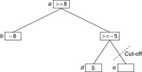
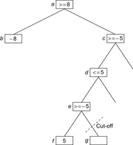
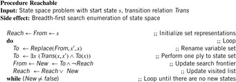
We consider shallow cut-offs first. Consider the situation in Figure 12.7, where one child has value −8. Then the value of the root will be at least 8. Subsequently, the value of node d is determined as 5, and hence node c achieves at least −5. Therefore, the player at the root would always prefer moving to b, and the outcome of the other children of c is irrelevant.
In deep pruning, the bound used for the cut-off can stem not only from the parent, but from any ancestor node. Consider Figure 12.8. After evaluating the first child f of e, its value must be −5 or larger. But the first player can already achieve 8 at the root by moving to b, so he will never choose to move to e from d, and the remaining unexplored children of e can be pruned. The implementation of αβ-search is shown in Algorithm 12.3.
For any node u, β represents an upper bound that is used to restrict the node below u. A cut-off occurs when it is determined that u's negmax value is greater than or equal to β. In such a situation, the opponent can already choose a move that avoids u with a value no greater than β. From the opponent's standpoint, the alternate move is no worse than u, so continued search below p is not necessary. We say that u is refuted. It is obvious how to extend αβ-pruning to minimax search (see Alg. 12.4).
The so-called fail-safe version of αβ initializes the variable res with −∞, instead of with α. This modification allows the search for the case where the initial window is smaller than (−∞, ∞) to be generalized. If the search fails (i.e., the root value lies outside this interval), an estimate is returned that informs us if the true value lies below α, or above β.
Theorem 12.1
(Correctness of Minimax Search with αβ-Pruning) Let u be an arbitrary position in a game and α < β. Then the following three assertions are true.
1.  .
.
2.  .
.
3.  .
.

Proof
We only proof the second assertion—the others are inferred analogously. Let u be a MAX node. We have  if and only if there exists a successor with res ≥ β. Since for all further successors we have that the value res only increases and res for the chosen state is the maximum of all previous res values including α, we conclude that res for the chosen state is equal to
  for some value res′ < res. By using induction we have that
  .
.
For the opposite direction we assume that  , which means that for all successors the value res is smaller than β. Therefore, the value val for all successors is smaller than β and
  .
.
An example of minimax game tree search with αβ pruning is shown in Fig. 12.9. In addition, the positive effect of pruning when additionally applying move ordering is illustrated.

Performance of αβ-Pruning
To obtain a bound on the performance of αβ-pruning, we have to prove that for each game tree there is a minimal (sub)tree that has to be examined by any search algorithm, regardless of the values of the terminal nodes. This tree is called the critical tree, and its nodes are critical nodes. It is helpful to classify nodes into three types, called PV, CUT, and ALL. The following rules determine critical nodes.
• The root is a PV node.
• The first child of a PV node is a PV, the remaining children are CUT nodes.
• The first child of a CUT node is an ALL node.
• All children of an ALL node are CUT nodes.
If we do not implement deep cut-offs, only three rules for determining the minimal tree remain.
• The root is a PV node.
• The first child of a PV node is also a PV, the remaining children are CUT nodes.
• The first child of a CUT node is a PV node.
The number of terminal leaves on the critical tree of a complete, uniform b-ary subtree of height d is This can also be motivated as follows. To prove that the value of the root is at least v, b⌈d/2⌉ leaves must be inspected, since one move must be considered on each player level, and all moves on each opponent level (this subtree is also called the player's strategy). Conversely, to see that the value is at most v, b⌊d/2⌋ − 1 leaf nodes have to be generated (the opponent's strategy). The principal variation lies in the intersection of the two.
If the tree is searched in best-first order (i.e., the best move is always chosen first for exploration), then αβ will search only the critical tree. Thus, for the performance of this algorithm it is crucial to apply move ordering (i.e., sorting the moves heuristically according to their expected merit).
Note that the preceding term is approximately  , where n = bd is the number of leaves in the whole (unpruned) tree. Consequently, we can state that αβ-pruning has the potential to double the search depth.
Extending Pruning to the Static Evaluator
Depending on its complexity, the static evaluation can claim most of the computational effort in game tree search. One idea to cut down on unnecessary overhead is to extend αβ-pruning into the evaluation itself. It is no longer considered an atomic operation. For example, in a weighted sum type of the evaluator, one feature is computed at a time, and a partial estimate is available at each step. Suppose that, as is usually the case, all feature values and weights are positive. Then, as soon as the partial sum exceeds the αβ-search window, we can discard the position without taking the remaining features into consideration.
This type of pruning is particularly powerful if the heuristic is represented in the form of a tree. Each internal node in a decision tree contains a test condition (e.g., an attribute comparison with a threshold value) that determines which branch to descend next. Its leaves contain the actual outcome of the evaluation. Decision trees can be automatically induced from labeled training examples. One drawback is that if an attribute is close to a threshold value, the evaluation can abruptly jump based on an arbitrary change in the input feature. As a remedy, generalizations of decision trees have been developed and have been applied to game playing that make the decision boundary “soft” or “fuzzy.”
12.1.3. Transposition Tables
As in single-agent search, transposition tables (see Sec. 6.1.1) are memory-intense dictionaries (see Ch. 3) of search information for valuable reuse. They are used to test if the value of a certain state has already been computed during a search in a different subtree. This can drastically reduce the size of the effective search game tree, since in two-player games it is very common to have different move sequences (or different orders of the same moves) lead to the same position.
The usual implementation of a transposition table is done by hashing. For fast hash function evaluations and large hash tables to be addressed a compact representation for the state is suggested.
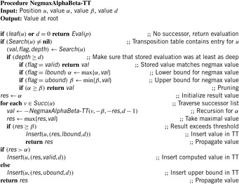
We apply transposition table lookup to the negmax algorithm with αβ-pruning. Algorithm 12.5 provides a suitable implementation. To interpret the different stored flags, recall that in the αβ-pruning scheme not all values of α and β yield the minimax value at its root. There are three sets to be distinguished: valid, the value of the algorithm matches the one of negmax search; lbound, the value of the algorithm is a lower bound for the one of negmax search; and ubound, the value of the algorithm is an upper bound for the one of negmax search.
In addition, note that the same position can be encountered at different depths of the tree. This depth is also stored in the transposition table. Only if the stored search depth is larger or equal to the remaining search depth can the result replace the execution of the search.
Major nuances of the algorithm concern the strategy of when to overwrite an entry in the transposition table. In Algorithm 12.5, the scheme “always replace” is used, which simply overwrites anything that was already there. This may not be the best scheme, and in fact, there has been a lot of experimental work trying to optimize this scheme. An alternative scheme is “replace if same depth or deeper.” This leaves a currently existing node alone unless the depth of the new one is greater than or equal to the depth of the one in the table.
As explained in the exposition of αβ-pruning (see Sec. 12.1.2), searching good moves first makes the search much more efficient. This gives rise to another important use of transposition tables, apart from eliminating duplicate work; along with a position's negmax value, it can also store the best move found. So if you find that there is a “best” move in your hash element, and you search it first, you will often improve your move ordering, and consequently reduce the effective branching factor. Particularly, if an iterative-deepening scheme is applied, the best moves from the previous, shallower search iteration tend to also be the best ones in the current iteration.
The history heuristic is another technique of using additional memory to improve move ordering. It is most efficient if all possible moves can be enumerated a priori; in Chess, for instance, they can be stored in a 64 × 64 array encoding the start and end squares on the board. Regardless of the exact occurrence in the search tree, the history heuristic associates a statistic with each move about how effective it was in inducing cut-offs in the search. It has been proven that these statistics can be used for very efficient move ordering.
12.1.4. *Searching with Restricted Windows
Aspiration Search
Aspiration search is an inexact approximation of αβ with higher cut-off rates. αβ-pruning uses an initial window  such that the game theoretical value is eventually found. If we initialize the window to some shorter range, we can increase the probability of pruning. For example, we can use a window
  , where v0 is a static estimate of the root value. If the bounds are chosen so large that for any position with a value at least that big we can be sure that it is won, then the exact outcome doesn't matter anymore. Alternatively, if the window was chosen too small, the fail-safe modification of αβ will return an improved bound α′ or β′ for either α or β, and a re-search has to be conducted with an appropriately enlarged window (α′, ∞) or (−∞, β′). The hope is that the increased pruning outweighs the overhead of occasional repeated searches.
Null-Window Search
A special case of this algorithm is the so-called null-window search. Using the fact that the values of α and β are integral, the initial window is set to (α − 1, α), so that no possible values lie between the bounds. This procedure will always fail, either low or high; it can essentially be used to decide whether the position is below or above a given threshold. Null-window search is mostly used as a subroutine for more advanced algorithms, as described in the following.
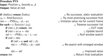
Principal-Variation Search
Principal-variation search (see Alg. 12.6) is based on the same rationale as aspiration search; that is, it is attempting to prune the search tree by reducing the evaluation window as much as possible. As soon as the value for one move has been obtained, it is assumed that this move is indeed the best one; a series of null-window searches is conducted to prove that its alternatives are inferior. If the null-window search fails high, then the search has to be repeated with the correct bounds.
Memory-Enhanced Test Framework
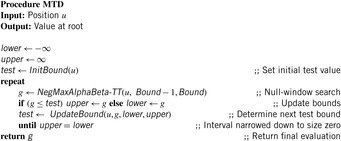
In contrast to principal-variation search, this class of algorithms relies only on a series of null-window searches to determine the negmax value of a position. The general outline of the framework is shown in Algorithm 12.7. It requires the programmer to implement two functions: InitBound calculates the test bound used in the first null-window search and UpdateBound does so for all successive iterations, depending on the outcome of the last search. The aim is to successively refine the interval (lowerBound, upperBound) in which the true negmax value lies, as fast as possible. To offset the cost of repeated evaluations, a transposition table is used.
One particular instantiation is called MTD(f). It uses the following procedure to update the bound: That is, the new bound obtained from the last null-window search is used to split the interval.
It is clear that starting with an initial guess closer to the real negmax value should reduce the number of iterations and lead to faster convergence. One way to obtain such an estimate would be to use the static evaluation. Better yet, if, as usual, an iterative-deepening scheme is applied, the result of the previous shallower search can be exploited in InitBound.
Apart from MTD(f), other possible instantiations of the MTD framework include:
MTD(∞): InitBound returns ∞, UpdateBound sets testBound to g. While MTD(f) can be called realistic, this procedure is optimistic to the extent that it successively decreases an upper bound.
MTD(bi): UpdateBound sets testBound to the average of lowerBound and upperBound to bisect the range of possible outcomes.
MTD(step): Like in MTD(∞), an upper bound is successively lowered. However, by making larger steps at a time, the number of searches can be reduced. To this end, UpdateBound sets testBound to max(lower + 1, g − stepsize).
Best-First Search
For over a decade prior to the introduction of the MTD framework, best-first search for two-player games had been shown to have theoretical advantages over the αβ-procedure. Like A*, the algorithm SSS* maintains an Open list of unexpanded nodes; as governed by a set of rules, in each step the node with the best evaluation is selected, and replaced by a number of other nodes, its children or its parent. In some cases, Open has to be purged of all ancestors of a node.
It was proven that in a statically ordered game tree, SSS* dominates αβ in the sense of the number of evaluated leaf nodes that cannot be higher, and is often significantly lower. However, the algorithm never played a practically relevant role due to a number of perceived shortcomings:
• From the original formulation, the algorithm is hard to understand.
• It has large memory requirements.
• Purging of ancestor nodes is slow.
These problems could still not be completely overcome by subsequently developed improvements and variations, such as a recursive formulation, and an algorithm, which in analogy to SSS* successively increases a lower bound on the negmax value.
Now, with the advent of the MTD framework described in the previous section, a surprising breakthrough in game tree search research was achieved by clarifying the relation between the previously incomparable and disparate approaches of depth-first and best-first search. Specifically, with a sufficiently large transposition table, MTD(∞) and SSS* are equivalent to the extent that they expand the same nodes, in the same order. Since MTD only adds one loop around standard αβ-search, it is easy to see that the reason why SSS* can expand less leaf nodes is that searching with a null window allows for considerably more pruning. The memory requirements can be flexibly alleviated in dependence of available main memory by allocating less space for the transposition table (though it might be argued that this objection to SSS* is no longer valid for modern-day computers). No expensive priority queue operations are needed in the implementation, and the transposition table is usually realized as a hash table, resulting in constant-time access.
An experimental comparison of different depth-first and best-first algorithms on realistic game situations in Checkers and Chess was conducted. All algorithms were given the same memory constraints. The results contradicted a number of previously held beliefs. MTD(f) turned out to consistently outperform other algorithms, both in terms of expansion numbers and execution times. SSS* yields only a modest improvement over αβ, and is sometimes outperformed both by depth-first and best-first algorithms. One reason is that the dominance proof of SSS* over αβ assumes static move ordering; when, in an iterative-deepening scheme, a transposition table is used to explore the best moves from the previous iteration first, the latter algorithm can beat the former one. Contradicting earlier results with artificially generated trees, best-first search is generally not significantly better than depth-first search in practice, and can sometimes be even much worse. The reason is that additional, commonly applied search enhancements (some of which will be briefly discussed) are very effective in improving efficiency and reducing their advantage.
Another important lesson learned from the empirical algorithm comparison is that with search enhancements on realistic situations, the efficiency of all algorithms differed only by at most around 10%. Thus, we can say that the search enhancements used in high-performance game playing programs improve the search efficiency to an extent close to the critical tree, such that the question of which algorithm to use is no longer of prime importance.
12.1.5. Accumulated Evaluations
In some domains (e.g., some card games), the total evaluation at a leaf is in fact the sum of the evaluation at interior nodes. In this case, the αβ-routine for minimax search has to be implemented with care. The problem of usual αβ-pruning is that the accumulated value that will be compared in a transposition table lookup is influenced by the path. Algorithm 12.8 shows a possible implementation for this case.
Theorem 12.2
(Correctness αβ for Accumulated Estimates) Let u be any game position. Then we have
12.1.6. *Partition Search
Partition search is a variation of αβ-search with a transposition table. The difference is that the transposition table not only contains single positions, but entire sets of positions that are equivalent.
The key observation motivating partition search is the fact that some local change in the state descriptor does not necessarily change the possible outcome. In Chess, a checkmate situation can be independent of whether a pawn is on a5 or a6. For card games, changing two (possibly adjacent) cards in one hand can result in the same tree. First, we impose an ordering ≺ on the set of individual cards, then two cards c and c′ are equivalent with respect to hands of cards C1, and C2, if  , and for all
  we have
  if and only if
  .
.
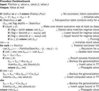
The technique is contingent on having available an efficient representation for the relevant generalization sets. These formalisms are similar as in methods dealing with abstract search spaces (see Ch. 4). In particular, we need three generalization functions called P, C, and R, that map a position to a set. Let U be the set of all states, S ⊆ U a set, and u ∈ U.
•  maps positions to sets such that
  ; moreover, if u is a leaf, then Eval(u) = Eval(u′) for each
  (i.e., P is any generalization function respecting the evaluation of terminal states).
•  maps a position and a set to a set. It must hold that
  , if some position in S is reachable from u; moreover, every
  must have some successor in S (i.e., R is a generalization of u that contains only predecessors of states in S).
Note that if all states in a set S have a value of at least val, then this is also true for R(p, S); analogously, an upper bound for the value of positions in S is also an upper bound for those in C(p, S). Combining these two directions, if Sall denotes a superset of the successors of a position u with equal value, and Sbest is a generalization of the best move with equal value, then all states in  will also have the same value as u. This is the basis for Algorithm 12.9.
In the game of Bridge, partition search has been empirically shown to yield a search reduction comparable to and on top of that of αβ-pruning.

12.1.7. *Other Improvement Techniques
During the course of the development of modern game playing programs, several refinements and variations of the standard depth-first αβ-search scheme have emerged that greatly contributed to their practical success.
• A common drawback of searching the game tree up to a fixed depth is the horizon effect: If the last explored move was, for example, a capture, then the static evaluation might be arbitrarily bad, ignoring the possibility that the opponent can take another piece in exchange. The technique of quiescence search, therefore, extends evaluation beyond the fixed depth until a stable or quiescent position is reached. Apart from null moves, where a player essentially passes, only certain disruptive moves are taken into consideration that can significantly change the position's value, such as captures.
• Singular extension increases the search depth at forced moves. A MAX position p with depth d value v is defined to be singular if all of its siblings p′ have a value at most v − δ, for an appropriately chosen margin δ. Singular extensions are considered crucial in the strength of world-champion Chess program Deep Thought.
• Conspiracy search can be seen as a generalization of both quiescence search and singular extensions. The basic rationale behind this approach is to dynamically let the search continue until a certain confidence in the root value has been established; this confidence is measured by the number of leaf nodes that would have to “conspire” to change their value to bring the strategy down. Thus, the higher the conspiracy number of a node, the more robust is its value to inaccuracies in the static evaluation function. The tree can be searched in a way that aims to increase the conspiracy number of the root node, and thus the confidence in its value, while expanding as few nodes as possible.
The ABC procedure works similarly as αβ, except that the fixed-depth threshold is replaced by two separate conspiracy-depth thresholds, one for each player. The list of options is recursively passed on to the leaves, as an additional function argument. To account for dependencies between position values, the measure of conspiracy depth can be refined to the sum of an adjustment function applied to all groups of siblings. A typical function should exhibit “diminishing return” and approach a maximum value for large option sets. For the choice of the constant function, the algorithm reduces to ordinary αβ-search as a special case.
• Forward pruning refers to different cut-off techniques to break full-width search at the deepest level of the tree. If it is MAX's turn at one level above the leaves, and the static evaluation of the position is already better than β, the successor generation is pruned; the underlying assumption is that MAX's move will only improve the situation in his favor. Forward pruning might be unsafe because, for example, zugzwang positions are ignored.
• Interior-node recognition is another memorization technique in game playing that includes game theoretical information in the form of score values to cut-off whole subtrees for interior-node evaluation in αβ-search engines. Recognizers are only invoked, if transposition table lookups fail.
• Monte Carlo search (random game play) is an upcoming technique currently used with some success in 9 × 9 Go. Instead of relying on a heuristic to rank the moves that are available in a position (and then choosing the best one), their value is derived from a multitude of simulated, complete games starting from that position that the computer plays against itself.
Before starting to play, the players form an ordered list of all available moves they are going to play. Then, in turn-taking manner they execute these moves regardless of the opponent's moves (unless it is not possible, in which case they simply skip to the subsequent one). The underlying assumption is made that the quality of the moves can be assessed independently of when they are played. Although this is certainly an oversimplification, it often holds in many games that a good move at one ply stays a good one two plys ahead. 1 The value of a move is the average score of the matches in which it occurred, and is updated after each game.
1We could call this the zero-order algorithm. The first-order algorithm would record the value of the move dependent on the preceding move of the opponent, and so on. On the flip side, this also increases drastically the number of games that need to be played to reach an acceptable accuracy.
When generating the move list, first, all moves are sorted according to their value. Then, in a second pass, each element is swapped with another one in the list with a small probability. The probability of shifting n places down the list is  where T is the so-called temperature parameter that slowly decreases toward zero between games. The intuition behind this annealing scheme is that in the beginning, larger variations are allowed to find the approximate “geographical region” of a good solution on a coarse scale. As T becomes smaller, permutations become less and less likely, allowing the solution to be refined, or, to use the spatial analogy, to find the lowest valley within the chosen region. In the end, the sequence is fixed, and the computer actually executes the first move in the list.
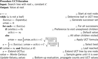
• The UCT algorithm is a value-based reinforcement learning algorithm. The action value function is approximated by a table, containing a subset of all state-action pairs. A distinct value is estimated for each state and action in the tree by Monte Carlo simulation. The policy used by UCT balances exploration with exploitation. UCT has two phases. In the beginning of each episode it selects actions according to knowledge contained within the search tree (see Algorithm 12.10). But once it leaves the scope of its search tree it has no knowledge and behaves randomly. Thus, each state in the tree estimates its value by Monte Carlo simulation. As more information propagates up the tree, the policy improves, and the Monte Carlo estimates are based on more accurate returns. Let n(u, a) count the number of times that action a has been selected from state u (initialized to 1 on the first visit). Let  be a simulated path in which—if present—unused actions are chosen uniformly, and—if all applicable actions have been selected—preferred by the q-value. The updates are
  , and
, and  , where rt is a constant to which q(u, a) is also initialized. For two-player games, under some certain assumptions, UCT converges to the minimax value without using any prior knowledge on the evaluation function. UCT also applies to single-agent state space optimization problems with large branching factors (e.g., Morpion Solitaire and Same Game, see Exercises).
• In some multiplayer games or games of incomplete information like Bridge we can use Monte Carlo sampling to model the opponents according to the information that is available. An exact evaluation of a set of samples for a given move option then gives a good decision procedure. The sampling approach is often implemented by a randomized algorithm that generates partial states efficiently. The drawback of sampling is that it cannot deal well with information-gathering moves.
12.1.8. Learning Evaluation Functions
As mentioned before, a crucial part of building good game playing programs lies in the design of the domain-specific evaluation heuristic. It takes a lot of time and effort for an expert to optimize this definition. Therefore, from the very beginning of computer game playing, researchers tried to automate some of this optimization, making it a testbed for early approaches to machine learning. For example, in the common case of an evaluation function being represented as a weighted sum of specialized feature values, the weight parameters could be adjusted to improve the program's quality of play based on its experience of previous matches. This scenario is closely related to that of determining an optimal policy for an MDP (see Sec. 1.8.3), so it will not come as a surprise that elements like the backup of estimated values play a role here, too. However, MDP policies are often formulated or implicitly assumed as a big table, with one entry for each state. For nontrivial games, this kind of rote learning is infeasible due to the huge number of possible states. Therefore, the static evaluator can be regarded as an approximation of the complete table, mapping states with similar features to similar values. In the domains of statistics and machine learning, a variety of frameworks for such approximators have been developed and can be applied, such as linear models, neural networks, decision trees, Bayes networks, and many more.
Suppose we have a parametric evaluation function Evalw(u) that depends on a vector of weights  , and a couple of training examples
  supplied by a teacher consisting of pairs of positions and their “true” value. If we are trying to adjust the function so that it comes as close as possible to the teacher's evaluation, one way of doing this would be a gradient descent procedure. The weights should be modified in small steps, such as to reduce the error E, measured, for example, in terms of the squared differences
  between the current output and the target value. The gradient ∇wE of the error function is the vector of partial derivatives, and so the learning rule could be to change w by an amount,
 with a small constant α called the learning rate.
Supervised learning requires a knowledgeable domain expert to provide a body of labeled training examples. This might make it a labor-intensive and error-prone procedure for training the static evaluator. As an alternative, it is possible to apply unsupervised learning procedures that improve the strategy while playing games against other opponents or even against themselves. These procedures are also called reinforcement learning, for they are not provided with a given position's true value—their only input is the observation of how good or bad the outcome is of a chosen action.
In game playing, the outcome is only known at the end of the game, after many moves of both parties. How do you find out which one(s) of them are really to blame for it, and to what degree? This general issue is known as the temporal credit assignment problem. A class of methods termed temporal difference learning is based on the idea that successive evaluations in a sequence of moves should be consistent.
For example, it is generally believed that the minimax value of a position u, which is nothing other than the backed-up static evaluation value of positions d moves ahead, is a more accurate predictor than the static evaluator applied to u. Thus, the minimax value could be directly used as a training signal for u. Since the evaluator can be improved in this way based on a game tree determined by itself, it is also a bootstrap procedure.
In a slightly more general setting, a discounted value function is applied: executing an action a in state u yields an immediate reward w(u, a). The total value fπ(u) under policy π is  , where a is the action chosen by π in a, and v is the resulting state. For a sequence of states u0, u1, and so on, chosen by always following the actions a0, a1, and so on prescribed by π, the value is equal to the sum
 The optimal policy π* maximizes the f*-value.
An action-value function Q*(u, a) is defined to be the total (discounted) reward experienced when taking action a in state u. It is immediate that  . Conversely, the optimal policy is
  .
.
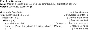
Temporal difference learning now starts with an initial estimate Q(u, a) of Q*(u, a), and iteratively improves it until it is sufficiently close to the latter (see Alg. 12.11). To do so, it repeatedly generates episodes according to a policy π, and updates the Q-estimate based on the subsequent state and action.
In Figure 12.10 (left) we have displayed a simple directed graph with highlighted start and goal nodes. The optimal solution is shown to its right. The costs (immediate rewards) assigned to the edges are 1,000 in case it is the node with no successor, 0 in case it is the goal node, and 1 if it is an intermediate node.
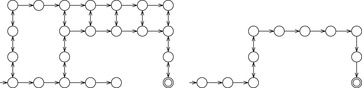
Figure 12.11 displays the (ultimate) effect of applying temporal difference learning or Q-learning. In the left part of the figure the optimal value function is shown, and on the right part of the figure the optimal action-value function is shown (upward/downward cost values are annotated to the left/right of the bidirectional arrows).
 |
| Figure 12.11 |
The TD(λ) family of techniques has gained particular attention due to outstanding practical success. Here, the weight correction tries to correct the difference between successive estimates in a consecutive series of position  ; basically, we are dealing with the special case that the discount factor δ is 1, and all rewards are zero except for terminal (won or lost) positions. A hallmark of TD(λ) is that it tries to do so not only for the latest time step, but also for all preceding estimates. The influence of these previous observations is discounted exponentially, by a factor λ:
 As the two extreme cases, when λ = 0, no feedback occurs beyond the current time step, and the formula becomes formally the same as the supervised gradient descent, but the target value is replaced by the estimate at the next time step. When λ = 1, the error feeds back without decay arbitrarily far in time.
Discount functions other than exponential could be used, but this form makes it particularly attractive from a computational point of view. When going from one time step to the next, the sum factor can be calculated incrementally, without the need to remember all gradients separately:
In Algorithm 12.11, the same policy being optimized is also used to select the next state to be updated. However, to ensure convergence, it has to hold that in an infinite sequence, all possible actions are selected infinitely often. One way to guarantee this is to let π be the greedy selection of the (currently) best action, except that it can select any action with a small probability ϵ. This issue is an instance of what is known as the Exploration-Exploitation Dilemma in Reinforcement Learning. We want to apply the best actions according to our model, but without sometimes making exploratory and most likely suboptimal moves, we will never obtain a good model.
One approach is to have a separate policy for exploration. This alley is taken by Q-learning (see Alg. 12.12). Note that
Finally, it should be mentioned that besides learning the parameters of evaluation functions, approaches have been investigated to let machines derive useful features relevant for the evaluation of a game position. Some logic-based formalisms stand out where inductive logic programming attempts to find if-then classification rules based on training examples given as a set of elementary facts describing locations and relationships between pieces on the board. Explanation-based learning was applied to classes of endgames to generalize an entire minimax tree of a position such that it can be applied to other similar positions. To express minimax (or, more generally, AND/OR trees) as a logical expression, it was necessary to define a general explanation-based learning scheme that allows for negative preconditions (intuitively, we can classify a position as lost if no move exists such that the resulting position is not won for the opponent).
12.1.9. Retrograde Analysis
Some classes of Chess endgames with very few pieces left on the board still require solution lengths that are beyond the capabilities of αβ-search for optimal play. However, the total number of all positions in this class might be small enough to store each position's value explicitly in a database. Therefore, many Chess programs apply such special-case databases instead of forward search. In the last decade, many of such databases have been calculated, and some games of low to moderate complexity have even been solved completely. In this and the following sections, we will have a look at how such databases can be generated.
The term retrograde analysis refers to a method of calculation that finds the optimal play for all possible board positions in some restricted class of positions (e.g., in a specific Chess endgame, or up to a limited depth). It can be seen as a special case of the concept of dynamic programming (see also Sec. 2.1.7). The characteristic of this method is that a backward calculation is performed, and all results are stored for reuse.
In the initialization stage, we start with all positions that are immediate wins or losses; all others are tentatively marked as draws, possibly to be changed later. From the terminal states, alternating win backup and loss backup phases successively calculate all won or lost positions in 1, 2, and further plies by executing reverse moves. The loss backup generates predecessors of states that are lost for the player in n plies; all of these are won for the opponent in n + 1 plies. Win backup requires more processing. It identifies all n-ply wins for the player, and generates their predecessor. For a position to be lost in n + 1 plies for the opponent, all of its successors must be won for the player in at least n plies. The procedure iterates until no new positions can be labeled. The states that could not be labeled won or lost during the algorithm are either drawn or unreachable; in other words, illegal.
It would be highly inefficient to explicitly check each successor of a position in the win backup phase. Instead, we can use a counterfield to store the number of successors that have not yet been proven a win for the opponent. If it is found to be a predecessor of a won position, the counter is simply decremented. When it reaches zero, all successors have been proven wins for the opponent, and the position can be marked as a loss.
12.1.10. *Symbolic Retrograde Analysis
In this section, we describe an approach to how retrograde analysis can be performed symbolically, following the approaches of symbolic search described in Chapter 7. The sets of won and lost positions are represented as Boolean expressions; efficient realizations can be achieved through BDDs.
We exemplify the algorithmic considerations to compute the set of reachable states and the game theoretical values in this set for the game of Tic-Tac-Toe. We call the two players white and black.
To encode Tic-Tac-Toe, all positions are indexed as shown in Figure 12.12. We devise two predicates: Occ(x, i) being 1 if position i is occupied, and Black(x, i) evaluating to 1 if the position i, 1 ≤ i ≤ 9 is marked by Player 2. This results in a total state encoding length of 18 bits. All final positions in which Player 1 has lost are defined by enumerating all rows, columns, and the two diagonals as follows.
The predicate BlackLost is defined analogously. To specify the transition relation, we fix a frame, denoting that in the transition from state s to s′, apart from the move in the actual grid cell i, nothing else will be changed. These predicates are concatenated to express that with respect to board position i, the status of every other cell is preserved.
 Now we can express the relation of a black move. As a precondition, we have that one cell i is not occupied; the effects of the action are that in state s′ cell i is occupied and black.
 The predicate WhiteMove is defined analogously.
To devise the encoding of all moves in the transition relation Trans(x, x′), we introduce one additional predicate Move, which it is true for all states with black to move. There are two cases. If it is black's turn and if he has not already lost, execute all black moves; the next move is a white one. The other case is interpreted as follows. If white has to move, and if he has not already lost, execute all possible white moves and continue with a black one.
Reachability Analysis
In general, not all positions that are expressible in the domain language are actually reachable from the initial state (e.g., no Tic-Tac-Toe position can occur where both white and black have three marks in a row). To make symbolic retrograde analysis more efficient, we can restrict attention to reachable states. Therefore, to prepare for this, we describe symbolic reachability analysis first.
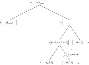
Essentially, it corresponds to a symbolic breadth-first search traversal, which successively takes the set From all positions in the current iteration and applies the transition relation to find the set of all New positions in the next iteration.
The algorithm terminates if no new position is available; that is, the expression for New is inconsistent. The union of all new positions is stored in the set Reached. The implementation is depicted in Algorithm 12.13.
Game-Theoretical Classification
As stated earlier, two-player games with perfect information are classified iteratively. Therefore, in contrast to reachability analysis, the direction of the search process is backward. Fortunately, backward search causes no problems, since the representation of all moves has already been defined as a relation.
Assuming optimal play and starting with all goal situations according to one player (here black's lost positions) all previous winning positions (here white's winning positions) are computed. A position is lost for black if all moves lead to an intermediate winning position in which white can force a move back to a lost position. This is also called a strong preimage. The choice of the actions ∧ for existential quantification (weak preimage) and ⇒ for universal quantification (strong preimage) are crucial.
The pseudo code for symbolic classification is shown in Algorithm 12.14. The algorithm Classify starts with the set of all final lost positions for black, and alternates between the set of positions that in which black (at move) will lose and positions in which white (at move) can win, assuming optimal play. In each iteration, each player moves once, corresponding to two quantifications in the analysis. The executed Boolean operations are exactly those established in the preceding recursive description. One important issue is to attach the player to move, since this information might not be available in the backward traversal. Furthermore, the computations can be restricted to the set of reachable states through conjunction. We summarize that given a suitable state encoding Config, for symbolic exploration and classification in a specific two-player game the programmer has to implement the procedures of the following interface.
1. Start(Config): Definition of the initial state for reachability analysis.
2. WhiteLost(Config): Final lost position for white.
3. BlackLost(Config): Final lost position for black.
4. WhiteMove(Config, Config): Transition relation for white moves.
5. BlackMove(Config, Config): Transition relation for black moves.

12.2. *Multiplayer Games
Most of the work in computer game playing research has focused on two-player games. Games with three or more players have received much less attention. Nearly all multiplayer games involve negotiation or coalition-building to some degree, which makes it harder to define what an “optimal” strategy consists of.
The value of a game state is formalized by a vector of size p, where component i denotes the value for player i. In turn-taking games at the root, it is the first player's turn to move; at the first level of the game tree, it is the second player's turn, and so on, until the sequence repeats after p levels. These trees are called Maxn-trees.
The negmax-search formulation is based on the zero sum assumption, and on the fact that with only two players, the score of one of them trivially determines the other one. Therefore, in the following we will stick to the minimax formulation. The basic evaluation procedure can be readily transferred to the case of multiple players: at each node, the player i to move chooses the one that maximizes the ith component of the score vector.
However, computational difficulties arise when trying to adopt two-player pruning strategies, such as αβ-search. More precisely, shallow pruning works in the same way if bounds on the maximum and minimum score of a player and of the total score can be provided; deep pruning, however, is not applicable.
Let minp and maxp be the minimum and maximum score any player can achieve, and minsum and maxsum be the minimum and maximum sum of the scores of all players. For zero-sum games, these two are equal. Figure 12.13 illustrates shallow pruning in an example with three players, and maxsum = 10. Player 1 can secure a value of 8 by moving from root a to b. Suppose subsequently node d is evaluated to a score of 3. Since Player 2 can score a 3 at c, both other players can achieve at most 10 − 3 = 7 for their components in the remaining unexplored children of c. Therefore, no matter what their exact outcome is, Player 1 will not choose to move to c, and hence they can be pruned.
The following lemma states that shallow pruning requires that the maximum achievable score for any player must be at least half of the maximum total score.
Lemma 12.1
Assume minp is zero. Then shallow pruning in a Maxn-tree requires maxp ≥ maxsum/2.
Proof
In Figure 12.13, denote the value for Player 1 at b as x, and that for Player 2 at d as y. A cut-off requires x being larger than the maximal achievable value at c, or x ≥ maxsum − y − (n − 2) ⋅ minp, which is equivalent to x + y ≥ maxsum using minp = 0. The claim follows from 2 ⋅ maxp ≥ x + y.
The asymptotic branching factor for Maxn with shallow pruning is  in the best case, where b is the branching factor without pruning. For a concrete game, the potential for pruning depends on the number of players and the values of maxp, minsum, and maxsum.
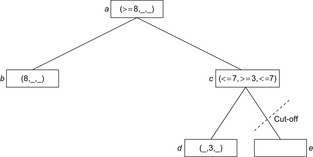
Let us now consider deep cut-offs. At first glance, following a similar argument as in the two-player case, the situation in Figure 12.14 should allow pruning all children of d but the first: Player 3 can achieve at least a value of 3, which leaves 7 for Player 1 at best, less than the 8 he can already achieve by moving from a to b. However, while the values of the other children of e cannot be the final outcome at the root, they can still influence the result. If the second child has the value (6, 0, 4), it will be selected by Player 3; at c, Player 2 will then prefer its right child e with value (9, 1, 0), which in turn yields the root value. In contrast, the branch would be irrelevant for the final outcome if Player 3 had selected the left child, f, instead.
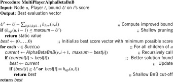
In the shallow pruning discussed earlier, we obtained an upper bound for Player 2 by subtracting the minimum achievable score for Player 1 from maxsum. But often we can give tighter values, when lower and/or upper bounds for all players are available. This is the case for examples in card games, where the number of tricks or the total value of card values in tricks is counted. A lower bound comes from the tricks a player has already won, and an upper bound from the outstanding cards left on the table; that is, those that have not yet been scored by another player.
A recursive formulation of the resulting algorithm is shown in Algorithm 12.15. It assumed two heuristic functions hlow(u, k) and hup(u, k) for lower and upper bounds on the score of player k in state u. The procedure performs shallow cut-offs based on a bound computed from the current best solution at the parent node.
As an alternative to Maxn, the tree evaluation can be reduced to the two-player case by making the paranoid assumption that all players form a coalition to conspire against the player at the root. This might result in nonoptimal play, however, reducing the search effort considerably. Player Max moves with a branching factor of b, while Min combines the rest of the players, and has therefore bp − 1 choices. The reduced tree has depth D = 2 ⋅ d/p, where d is the depth of the original tree. The best-case number of explored nodes is b(p−1)⋅D/2 for Max, and bD/2 for Min, which together results in  , or
, or  with respect to the original tree.
12.3. General Game Playing
In general game playing, strategies are computed domain-independently without knowing which game is played. In other words, the AI designer does not know anything about the rules. The players attempt to maximize their individual outcome. To enforce finite games, the depth is often bounded by using a step counter.
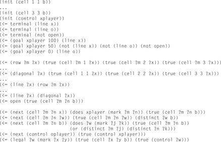
The game description language (GDL) is designed for use in defining complete information games. It is a subset of first-order logic. GDL is a Datalog-inspired language for finite games with discrete outcomes for each player. Broadly speaking, every game specification describes the states of the game, the legal moves, and the conditions that constitute a victory for the players. This definition of games is similar to the traditional definition in game theory with a couple of exceptions. A game is a graph rather than a tree. This makes it possible to describe games more compactly, and it makes it easier for players to play games efficiently. Another important distinction between GDL and classic definitions from game theory is that states of the game are described succinctly, using logical propositions instead of explicit trees or graphs. An example game in GDL notation is provided in Figure 12.15.
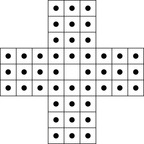
As another example, take the game Peg, of which the initial state is shown in Figure 12.16. On the board 32 pegs are located at the depicted locations. The player can move one peg by jumping over an occupied field onto an empty one. This jump may only be performed in a horizontal or vertical direction. The peg then moves to the formerly empty field, leaving the field where it started its jump empty. The peg that was jumped over is deleted from the board leaving its field empty, too. The game ends when no more jumps are possible. As with each jump one peg is removed, this situation arises after 31 jumps at the most. The main goal is to remove all pegs except for one. This then should be located in the very middle (i.e., we aim at the inverse of the initial state). This situation with 26,856,243 states is classified to receive 100 points. We also give certain points for other final states: 99 points for one remaining peg that is not in the middle (only 4 states receive this value), 90, …, 10 points for 2, …, 10 pegs remaining with respective 134,095,586; 79,376,060; 83,951,479; 25,734,167; 14,453,178; 6,315,974; 2,578,583; 1,111,851; and 431,138 states in the classification set. The remainder of 205,983 states have more than 10 pegs on the board.
Strategies for generalized game play include symbolic classification for solving, as well as variants of αβ and Monte Carlo and UCT search for playing the games.
12.4. AND/OR Graph Search
As before, we formalize a state space as a graph in which each node represents a problem state and each edge represents the application of an action. There are two conventional representations for AND/OR graphs, either with explicit AND and OR nodes, or as a hypergraph.
In the former representation, three different types of nodes exist. Apart from terminal (goal) nodes, interior nodes have an associate type, namely either AND or OR. Without loss of generality, we can assume that an AND node has only OR nodes as children, and vice versa; otherwise, we could transform it into one. As with regular search trees, edges can be assigned a weight, or cost. We will denote the cost of applying action a in state u (assuming it is applicable) as w(u, a). AND/OR graphs are commonly used in artificial intelligence to model problem reduction schemes. To solve a nontrivial problem, we decompose it to a number of smaller subproblems. Successfully solving the partial problems will produce a final solution to the original problem according to the decomposition conditions.
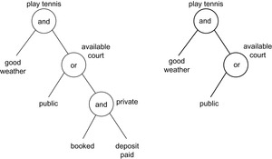
A simple example for an AND/OR graph is the following (see Fig. 12.17, left). To play tennis, two conjunctive conditions have to be satisfied: good weather and an available court. A court is either public or private. In the former case, there is no further requirement. If the playground is private, we have to book it and to pay a deposit.
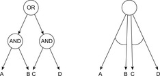
Hypergraphs are an equivalent formalization to AND/OR graphs. Instead of arcs that connect pairs of nodes, a hypergraph has hyperarcs that connect a node to a set of k nodes. The two representations can be transformed into each other by absorbing respectively inserting AND nodes, as Figure 12.18 demonstrates.
Both AND/OR graphs and hypergraphs can be interpreted in different ways. In the deterministic interpretation, an OR node corresponds to the type of nodes in ordinary search trees, in that it is sufficient to solve a single successor. In contrast, all successor states of an AND node have to be solved in turn and are necessary parts of an overall solution. On the other hand, in the framework of the Stochastic Shortest Path problem, an action is regarded as a stochastic action that transforms a state into one of several possible successor states according to some probability distribution: p(v|u, a) denotes the probability that applying action a to state u results in a transition to state v.
Because a hyperarc can have multiple successor states, AND/OR graph search generalizes the concept of a solution from a path to a tree (or, more generally, to a directed graph, if the same subgoal occurs in different branches). Starting from the initial state, it selects exactly one hyperarc for each state, each of its successors belong to the solution graph, in turn; each leaf is a goal node. The aim of the search algorithm is to find a solution tree (see Fig. 12.17, right) with minimal expected cost.
Recursively, a solution graph π satisfies the following properties. The root is part of the solution graph. Only one successor of an OR-node is contained in the solution graph. All of the successors of an AND node are part of π. The deepest directed paths must end with a goal node. The tennis example has two possible solution graphs.
In a solution graph, we can associate with each node the cost of solving the problem represented by that node. The cost of node u is defined by bottom-up recursion as follows. The cost f(u) of a goal node is 0. At an internal node, an action a is applied. We have  if v is a successor of an OR node u, and
 if u is an AND node. In the probabilistic interpretation, the latter formula becomes
 In other words, the objective of a minimum-cost solution is generalized to a solution with expected minimum cost, averaging over all possible outcomes of an action.
12.4.1. AO*
We now describe a heuristic search algorithm to determine the minimum-cost solution graph in an AND/OR tree. The algorithm starts with an initial node and then builds the AND/OR graph using the successor-generating subroutine Expand. At each time, it maintains a number of candidate partial solutions, which are defined in the same way as a solution, except that some tip nodes might not be terminal. To facilitate retrieval of the best partial solution, at each node the currently known best action is marked; it can then be extracted by following the marked edges top-down, starting at the root.
AO* as shown in Algorithm 12.16 works by repeatedly enlarging the best partial solution until a complete solution is found. The best partial solution is alleviated by associating with each iteration a nonterminal tip node from the currently best partial solution (which can be retrieved by following the marked paths from the root) that is selected for expansion. The f-value records a lower bound on the expected solution cost. For each successor, it is initialized with its h-value (or zero, for a goal state).
Eventually, the root becomes labeled as solved, in which case we obtain a minimum-cost solution graph by tracing down the marked edges. The performance of the algorithm depends on the informedness of the search heuristic.
Since the solution cost of a node depends on that of its successors, it has to be updated whenever the latter ones' estimate changes. Therefore, the algorithm interleaves forward expansion with a dynamic programming step that uses backup induction. The set Z of nodes possibly affected by the expansion of u consists of u and all its ancestors. More precisely, only those ancestors can change their value where u lies on a path of minimal cost. The nodes in Z are updated in an order so that all descendants of a node x are treated before x. In case of an OR node, we mark the edge that leads to the minimum heuristic estimate. In the case of an AND node, all edges are marked. Note that these updates can change the partial solution tree.
For sake of completeness, Algorithm 12.17 outlines the equivalent formalization of the AO* algorithm for a stochastic environment. This time, we provide the stochastic version, taking into account the probabilities  . The deterministic algorithm can be derived by simply setting them to 1. For brevity, the labeling of solved nodes is omitted.
Both Algorithm 12.16 and Algorithm 12.17 contain nondeterminism about which of the generally multiple terminal nodes of an optimal partial solution to choose for expansion. This choice will greatly affect the efficiency of the overall algorithm. Possible alternatives include the node with least cost, or with highest probability to be reached.
12.4.2. *IDAO*
Like IDA* does with A* for regular search graphs, it is similarly possible to devise an iterative-deepening variant of AO* to cope with AND/OR graphs. The approach exploits the fact that the value function often maps to a small integer. It reassembles ideas for IDA* from the deterministic case. The main driver loop of the IDAO* algorithm (see Alg. 12.18) triggers searches with successively increasing upper thresholds U.
The main difference to IDA* is the DFS subroutine (see Alg. 12.19). When expanding an AND node, it recursively invokes the main procedure rather than the DFS function. As a result, for each successor to an AND node, the IDAO* algorithm performs a series of searches with increasing cost bound, starting from the heuristic estimate of the successor node and ending when a solution is found or the cost bound of the predecessor AND node is reached. This is because we prefer cheaper partial solutions, even if the overall cost (determined by the maximum over all children) does not increase. The cost value returned is always a lower bound on the optimal cost of the expanded node, and equal to the optimal cost if the node is solved.
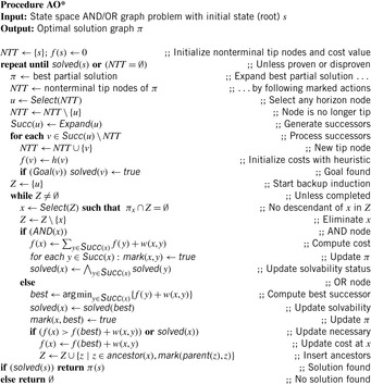
IDAO* stops searching the successors of an AND node as soon as one is found to have a cost greater than the current bound, since this implies the cost of the AND node to also increase the bound. However, since the algorithm performs repeated depth-first searches with increasing bounds, the entire problem will eventually be solved.
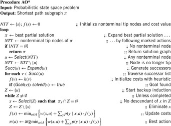
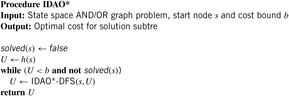
The algorithm shows how the f-value of a node can be made successively more accurate by backing up those of its children. When these improved bounds are stored in a transposition table that is always consulted prior to node expansion, the algorithm can be sped up considerably.
For brevity, we have not shown the reconstruction of the optimal solution. In contrast to AO*, this is performed in bottom-up fashion, starting at the leaves, and composing the solution from the partial solutions for the children at interior nodes. This could be implemented by augmenting the return value to comprise not only the cost of the solution, but the partial AND/OR tree as well.
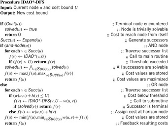
12.4.3. *LAO*
Unlike dynamic programming, heuristic search can find an optimal solution graph starting from a given state s without evaluating the entire state space. In light of the similarities to Markov decision processes, the question arises whether AND/OR graph search can be extended to this scenario for improved efficiency.
The major issue in the transferability concerns the existence of loops in MDPs. That is, after executing an action, there might be a nonzero chance of staying in the same state. A plan might have to repeat an action until it succeeds. As a consequence, MDPs are said to have an indefinite horizon, since no worst-case upper bound on the solution length can be ascertained.
LAO* is a simple generalization of AO* that can find solutions with loops (see Alg. 12.20). The key observation is that the backup-induction step of AO* can be regarded as a special case of dynamic programming, and hence, can be substituted by either policy iteration or value iteration (see Ch. 2). Like AO*, LAO* has two main steps: a forward search step and a dynamic programming step. The forward search step is the same as in AO*, except that it allows a solution graph to contain loops. Forward search of a partial solution graph now terminates at a goal node, a nonterminal tip node, or a loop back to an already expanded node.

For admissible estimates and policy iteration, LAO* has the following properties.
Theorem 12.3
(Optimality of LAO* for Policy Iteration) If h is admissible and policy iteration is used to perform dynamic programming in LAO*, then:
1. After each step for every state u we have f(u) ≤ f*(u).
2. After termination, for every state u in the best solution graph π, we have f(u) = f*(u).
3. LAO* terminates after a finite number of iterations.
Proof
The proof of the first assertion is by induction. Knowing that h is a lower bound, we have for every node u in the explicit graph an initial heuristic value h(u) ≤ f*(u). The forward search step expands the best partial solution graph and does not change the cost of any node and so it is sufficient to consider the dynamic programming step. For building an invariance condition, we make the inductive assumption that before the step, for every state u we have f(u) ≤ f*(u). If all tip nodes have optimal cost, then all the nontip nodes must converge to their optimal costs by the convergence for policy iteration. But by the induction hypothesis, all tip nodes have admissible costs. It follows that the nontip nodes must converge to costs that are as good or better than optimal when policy iteration is performed on them only.
To prove the second assertion, we observe that the search algorithm can only terminate if the solution graph is complete; that is, if it has no unexpanded nodes. For every state u in this solution graph it is contradictory to suppose f(u) < f*(u), since that implies a complete solution that is better than optimal. Together with Part 1 this yields f(u) = f*(u).
For proving the last assertion, it is clear that LAO* terminates after a finite number of iterations if the graph is finite, or equivalently the number of states in the MDP is finite.
For admissible estimates and value iteration algorithm LAO* can be proven to have similar properties.
Theorem 12.4
(Optimality of LAO* for Value Iteration) If h is admissible and value iteration is used to perform dynamic programming in LAO*, then:
1. After each step of LAO*, for every state u we have f(u) ≤ f*(u).
2. For every state u of the best solution graph π, we have f(u) converges to f*(u) in the limit.
Proof
The proof of the first assertion is also by induction. Knowing that h is a lower bound, for every node u in the explicit graph we have  . The hypothesis is that for every state u we have
  . If value iteration is performed, by restating the Bellman optimality equation we have
 To prove the second assertion, we observe that the graph is finite, so that LAO* must eventually find a complete solution graph. In the limit, the nodes in their solution graph must converge to their exact costs by the convergence proof for value iteration. The solution graph must be optimal by the admissibility of the costs of all the nodes in the explicit graph.
LAO* represents a solution as a mapping from states to actions in the form of a cyclic solution graph or, equivalently, a finite-state controller. The representation generalizes the graphical representations of a solution used by search algorithms like A* in the form of a simple path, and AO* in the form of an acyclic graph.
12.5. Summary
In this chapter, we generalized deterministic shortest path problems in different ways. Deterministic shortest path problems assume that the successor state is completely determined by the current state and the action executed in it. However, action executions can sometimes result in more than one successor state from which one is chosen during execution either probabilistically or by an adversary, in which case the search problem is either a probabilistic or minimax (respectively) shortest path problem and either the expected or worst-case (respectively) goal distances of the states must be found. The optimal behavior can, in both cases, be specified by the action that we should execute every time we are in a given state (policy).
We generalized these search problems to search problems with three different kinds of nodes: The first kind of nodes are the goal nodes. The have a given value. The second kind of nodes are called OR or, synonymously, MIN nodes. They are nodes where the MIN player picks one of the available actions. Their values are the minimum over all outgoing edges (i.e., actions) of the sum of the cost of moving to the successor node (i.e., the cost of executing the action) and the value of the successor Node. The third kind of nodes depends on the search problem: For probabilistic shortest path problems, they are called AVE nodes. They are nodes where nature picks one of the outcomes of the chosen action. Their values are the average over all outgoing edges (i.e., outcomes) of the sum of the cost of moving to the successor node (typically zero) and the value of the successor node.
We argued that probabilistic shortest path problems can be specified using Markov decision process (MDP) models with goal states. For minimax shortest path problems, the third kind of nodes are MAX nodes. MAX nodes are nodes where an adversary (the MAX player) picks one of the outcomes of the chosen action. Their values are the maximum over all outgoing edges (i.e., outcomes) of the sum of the cost of moving to the successor node (typically zero) and the value of the successor node. We also discussed AND/OR search problems, which are typically solved for tree-shaped state spaces only. For AND/OR search problems, the third kind of nodes are AND nodes. AND nodes are nodes where the chosen action is decomposed into several actions that all need to be executed. Their values are the sum over all outgoing edges of the sum of the cost of moving to the successor node and the value of the successor node.
We discussed ways of determining the values of all nodes for these search problems. For tree-shaped state spaces (of which the root node is the start node and the leaves are the goal nodes) this can be done by expanding every node once, starting at the goal nodes. An example is the minimax search method for minimax shortest path problems. Minimax shortest path problems can be solved with a Dijkstra-like search method that expands every node once, starting at the goal nodes, even for state spaces with more general topologies as long as there are only positive-cost cycles. The reason is that the optimal policy is acyclic if the values of all nodes are finite. However, probabilistic shortest path problems typically cannot be solved by expanding every node only once because there might be no optimal policy that is acyclic even if the values of all nodes are finite. We discussed several dynamic programming methods that can be used to solve probabilistic shortest path problems, including policy iteration, value iteration, and Q-learning, where Q-learning is not told about the outcomes and costs of the actions but needs to learn them by executing actions (reinforcement-learning problem). We also generalized these three search methods to probabilistic shortest path problems without goal nodes, by using discounting to guarantee that the values of the nodes are finite.
We discussed that we can often utilize the knowledge of the start node to avoid having to determine the values of all nodes. In this case, we can use heuristic search methods that generalize A*. They start at the start node and use heuristics to focus the search toward the goal nodes. Examples are AO* (and its iterative-deepening version to save memory) for AND/OR search problems and LAO* for MDPs. Table 12.1 summarizes the algorithms for this class. It denotes whether the pseudo code assumes a nondeterministic or probabilistic environment and whether the AND/OR structure is assumed to be a tree or a general graph. Last, but not least, we mention if the algorithms operate on a single source or on multiple sources.
We then applied our insights to two-person zero-sum games with complete knowledge of the current state (e.g., board configuration in Chess or Checkers), with a brief discussion of how to generalize the approaches to multiperson zero-sum games with complete and incomplete information. In two-person zero-sum games with complete knowledge of the current state, we try to find the best move for a player (typically assumed to be the MAX player) under the assumption that the opponent (MIN player) plays optimally, which is reasonable if we find a strong move since the move remains strong if the opponent does not play optimally. Thus, game playing problems are basically minimax shortest path problems where all action costs are zero. The goal states are the terminal states. Their value is, say, infinity for a win of the MAX player (i.e., loss of the MIN player) and minus infinity for a loss of the MAX player (i.e., win of the MIN player).
These minimax shortest-path problems can be solved with the minimax search method. Around goal states, we can simply calculate the correct values of the states offline (retrograde analysis) and store them in endgame databases. However, the state spaces are typically much larger than the available memory, thus we cannot store the values of all states. Instead, we perform a search each time the MAX player has to move, generating only part of the state space around the current state (local search space). The perimeter states of the local search space then become the goal states. Their values correspond to how favorable the state appears to be for the MAX player based on a static evaluation heuristic that can either be hand-coded or learned from experience with machine learning methods, including reinforcement learning methods. Larger local search spaces tend to help the minimax search method to discover misleading static evaluations and thus result in better decisions (although this is not guaranteed). The minimax search method is typically implemented with depth-first search and thus operates on trees that contain many states multiple times. It then uses transposition tables to detect that the value of a state has already been computed and thus does not need to be computed again, which makes it more efficient.
We discussed different ways of making it even more efficient by not evaluating the values of states that are unimportant because they cannot be reached during optimal play. The alpha-beta search method, for example, maintains an alpha value (i.e., the best value that the MAX player is guaranteed to achieve, initialized with the value of a loss of the MAX player) and a beta value (i.e., the best value that the MIN player is guaranteed to achieve, initialized with the value of a loss of the MIN player) during its minimax search. The value of the root node of the tree is then guaranteed to be between the alpha and beta value, and we do not need to calculate the value of a state for which the alpha value is not strictly smaller than the beta value. The alpha-beta search method calculates the same values as the minimax search method and thus executes the same actions, given the same local search spaces. However, it calculates the values of many fewer states and can thus search much larger local search spaces (namely trees of up to twice the depth if actions in states are evaluated in order of decreasing strength for the person to play in the state) in the same time as the minimax search method and thus select better actions than the minimax search method.
We also discussed variants of the alpha-beta search method that initialize the alpha and beta values differently and are then able to calculate the value of the root node exactly only if it is between the initial alpha and beta values. These variants include aspiration search, principal-variation search, and search using the memory-enhanced test framework. We discussed various other enhancements of the alpha-beta search method, including search methods that generalize over similar states, that use static evaluations that are vectors of values, and that avoid horizon effects by enlarging the local search space until the static evaluations are stable.
There are also other search methods, including best-first search methods, but they are more complex than these versions of the alpha-beta search method (basically a depth-first search method) without being much more efficient for games like Chess. Games with large branching factors (like Go), however, require fundamentally different approaches, for example, based on Monte Carlo search or problem decomposition. Games with probabilistic elements (e.g., Backgammon and other games that require you to roll dice) or incomplete information (e.g., many card games) can be solved with variants of the minimax or alpha-beta methods. For card games, for example, sampling the hands of the opponents based on the available information and then playing as if we knew their hands seems to be a promising approach that transforms the problem to one of complete information and allows us to use variants of the alpha-beta method.
Table 12.2 displays the basic game playing programs of this chapter. We denote if the traversal direction is forward or backward search, on how many players are usually modeled, and a typical game playing application scenario. Analyzing games of chance like Backgammon bridges the stochastic with game tree search. Moreover, we have attached the memory requirements, where d is the depth of the search tree and |T| is its size.
12.6. Exercises
12.1 Consider the state space of the game as  . A game has an initial state and some predicate goal to determine whether the game has come to an end. We assume that every path from the initial state to a final one is finite. For the set of goal states
  , we define an evaluation function
  , with −1 for a lost position, 1 for a winning position, and 0 for a drawing one. This function is extended to
  asserting a game theoretical value to each state in the game. Let Li be the set of lost positions for Player i,
  .
.
1. Define the sets L1 and L2 recursively assuming optimal play.
2. Let R be the set of all reachable states; with respect to the initial position and the rules of the game, define the set of draw games.
12.2 Represent the Connect 4 game efficiently and estimate the number of reachable states for board widths and heights in between 4 and 9.
12.3 In Hex, a goal pattern is a virtual connection between both sides of the board (see Fig. 12.19).
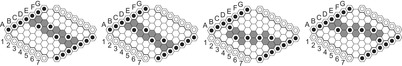
1. Show how to memorize goal patterns efficiently in an Unlimited Branching Tree (see Ch. 3). Insert the patterns of Figure 12.19 into the empty dictionary.
2. As illustrated in Figure 12.19 there are many further patterns that can be obtained through translation, reflection, and rotation. Determine the number of symmetries and insert all symmetric patterns in the example into the Unlimited Branching Tree.
12.4 In this partially completed Tic-Tac-Toe problem, both players were experts (neither one ever afforded the other an opportunity to force a win). What were the first and the last moves played?
 |
12.5 The key to the theory Nim is the digital binary sum neglecting all carryovers; for example, the sum for (011)2, (100)2, and (101)2 is (010)2. The optimal strategy is finishing every move with sum 0.
1. What is the optimal move for the configuration (3, 3, 5)?
2. Show that there is always a move from a situation with a digital sum ≠ 0 to one with a digital sum 0.
3. Show that every possible move in a situation with digital sum 0 makes the sum different to 0.
12.6 The most common implementation of an incremental hash function in game playing is Zobrist hashing. Given a board with n squares and p different types of pieces (including the blank) an array Z of size n × 2p is filled with random numbers. The hash number is the XOR over the occupied squares of the entire board. For a typical game, it can be computed incrementally.
If a piece is moved then an XOR of the current hash number with the Zobrist numbers for that piece corresponding to the two squares of the move is needed. For two-player games we often have to XOR in another random number for the side to move. Extend Zobrist hashing to capturing of pieces.
12.7 Provide the pseudo code for minimax-αβ with transposition table pruning.
12.8 The 2004 Chess world championship was almost won for Kramnik. However, Leko (playing black) won the Game 8 with very limited time, finding a brilliant move with regard to the board in Figure 12.21 (left), resulting in a win of black.
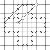
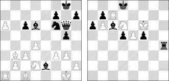
Now Leko was in the lead. But the last game was again won by Kramnik for a final outcome of 7:7. At the end he found a checkmate in at most three moves on the board in Figure 12.21 (right).
12.9 Morpion Solitaire is a pen-and-pencil game played on an infinite grid with some set S of a marked intersection taken as the initial state. In each move k − 1 intersections are covered and a new one is produced by placing a (horizontal, vertical, or diagonal) line having k − 1 edges. Edges of two lines must not overlap. The usual setting is S being a Greek cross with 36 = 6 ⋅ 4 + 6 ⋅ 2 marked intersections and k being 5 (see Figure 12.20). From a search perspective, Morpion Solitaire is a longest path state space problem. The best human solution of 170 moves dates back to April 1976. In 2010 a new record with 172 moves was obtained with Monte Carlo search and a grid computer.
1. Explain that the graph to be searched can be reduced to a tree.
2. Show that the game of the usual setting with k = 5 is finite.
3. Find a good state encoding and compare various bitmap encodings with line stacks.
4. Implement a breadth-first tree searcher. How deep can you go?
5. Implement a random depth-first tree searcher. What is the largest depth you find?
6. Apply UCT to the problem to trade exploitation with exploration.
12.10 Same Game is a single-agent game played on an n × m grid covered with nm balls in k colors. In the ordinary case, we have n = m = 15 and k = 5. Balls can be removed if they form a connected group of at least l elements. The reward of the move is (l − 2)2 points. If a group of balls is removed, others fall down. The goal of the game is to maximize reward. For total clearance, an additional reward of 1,000 points is given.
Speed-up Monte Carlo search.
1. Show that time O(nm) suffices to determine all valid successors of a grid state. (Propagate first the connectivity and then the sizes of the ball groups.)
2. Derive the concept of tabu colors that shouldn't be touched for a long time to form larger groups of balls. What would be a good color to select?
3. Given an evaluation function that assigns successors to positive values, derive a random choice model (think of a Roulette Wheel for weighted random choices).
4. What are good evaluation functions? Try to trade execution time with quality.
12.11 Skat is a popular three-player card game played on a 32 deck, where after bidding one player plays the other two. After bidding, computer Skat can be played on a double-dummy strategy that traverses a two-player search tree strategy grouping the two opponents together. (To determine the strength of a hand, Monte Carlo simulation has to be put on top of the double-dummy solver.)
1. Find out how Skat is played; that is, denote the value of each card and the rules of the game.
2. Find a 32-bit encoding for a hand, illustrate how to reverse the mapping, and determine a card-to-index procedure that allows you to efficiently determine if a card is better than another.
3. Explain how a card can be selected in O(1) and on modern computers by computing the most significant bit.
4. Analyze the following game of seven cards (♣ is trump, player 1 to play first.):
Player 1: ♣J ♣10 ♡8 ♡K ♡10 ♠7 ♠K
Player 2: ♠J ♡J ♣8 ♢9 ♢Q ♢10 ♢A
Player 3: ♣7 ♣Q ♢7 ♠8 ♠9 ♡7 ♡A
12.12 Apply symbolic retrograde analysis to Tic-Tac-Toe by using a symbolic model checking tool (e.g., SMV or μcke).
12.13 Blackjack is a card game, where a player tries to beat the dealer by obtaining a sum of card values that is higher than the dealer's. The limit is 21. The dealer stops hitting at 17. Explain how Blackjack can be solved with Q-learning. As the input, take the number of episodes for training, the number of games played per episode, the reinforcement values for a lost or won game, the step-size parameter, and the discount factor. Use epsilon-greedy for action selection. Higher epsilon values indicate higher exploration. Display the percentage of win games and the current learned Q-values.
12.14 In Tetris the player is continually given pieces of varying shapes that must be positioned and rotated, then dropped on the pieces below. The shape of each subsequent piece is random. Since pieces begin to pile up, the player must try to stack them efficiently. If the player manages to complete a row, then that row disappears, freeing up more space. Describe a reinforcement strategy to learn to play Tetris without directly programming its strategies. When given a random piece to add, it evaluates all the valid placements and chooses the action that results in the best one according to the evaluation function. Vary the value learning parameter and compare the efficiencies of Q-learning with temporal difference learning.
12.7. Bibliographic Notes
Good introductions to game theory have been given by Osborne and Rubinstein (1994) and by Owen (1982) and a general introduction to two-person game theory is found in the book by Rapoport (1966). Computer game playing goes back to the pioneer of computer science as a discipline (Turing et al., 1953) and the founding of information theory (Shannon, 1950). In 1950, Turing wrote the first computer chess program. The same year he proposed the Turing test, that in time, a computer could be programmed (e.g., playing Chess) to acquire abilities rivaling human intelligence. If a human did not see the other human or computer during an imitation game such as chess, he or she would not know the difference between the human and the computer.
There is some variance in notation in literature in writing Negmax/Negamax and MinMax/MiniMax. The idea of Neg(a)max results from a simplification reported by Baudet (1978). Several enhancements to αβ search including the history heuristic by Schaeffer (1989) have been proposed. Marsland and Reinefeld (1993) have treated principal-variation search. Plaat, Schaeffer, Pijls, and de Bruin (1996) have covered the MTD framework and its applications. SSS* has been proposed in Stockman (1997). Anantharaman, Campbell, and Hsu (1990) have described the concept of singular extensions. Classification tree and regression trees have been discussed by Breiman, Friedman, Olshen, and Stone (1984). Their application to αβ evaluation functions has been discussed by Heinz and Hense (1993). It has been proven that evaluation functions can exhibit some pathologies; see, for example, work by Nau (1983). Best-first minimax search, proposed by Korf and Chickering (1994), has clearly enhanced the quality of an Othello player. Generalization to αβ-search and SSS* have been discussed by Ibaraki (1986).
Conspiracy number search by McAllester (1988) and McAllester and Yuret (2002) search the game tree in a manner that several leaf evaluations have to change in order to change the root evaluation. Proof-number search, introduced by Allis, van der Meulen, and van den Herik (1994), proves or disproves the game-theoretical value. For this aim, it assigns a value to the root and shows that this value is equal to the minimax value. In every node, a proof number (and a disproof number) is stored that denotes the number of successors that have at least to be examined to prove (or disprove) the value. As proof-number search always considers the node with the largest influence on the root it is a best-first variant (with linear storage requirements). Proof-set search is a recent improvement to proof-number search, that trades node explorations for a higher memory consumption (Müller, 2002).
Samuel (1959) was the first researcher to implement a chess-playing program to apply learning in a game, and it was demonstrated on TV. His minimax algorithm included many heuristic extensions and cutoffs that we would call today αβ-pruning. He was also the first to use machine learning for improving the evaluation function, as a precursor of temporal-difference learning. The program played many thousand games against different versions of itself, and adjusted the weight parameters so as to approximate the minimax value of the position that resulted after two real plies in the match. TD(λ) has been proposed by Sutton (1988). It is an extension of TD(0) on so-called eligibility traces. The most impressive application of TD(λ) was Tesauro's TDGammon (1995) that is estimated to play close to the level of the best human players. Monte Carlo Go has been implemented by Bruegmann (1993) and has been played respectably on 9 × 9 Go. Most successful Go programs use UCT, as invented by Kocsis and Szepesvári (2006). UCT itself goes back to work by Auer, Cesa-Bianchi, and Fischer (2002). Known Go programs refer to initial work by Gelly and Silver (2007) and Coulom (2006).
Schrödl (1998) has introduced negation as failure to explanation-based learning and has used it to derive generalized logical descriptions of minimax trees for the chess endgame king-rook versus king-knight and could achieve up to 10-fold speedups.
A comprehensive reference for combinatorial game theory is contained in the book Winning Ways by Berlekamp, Conway, and Guy (1982), in which games are split into a sum of local games of tractable size. The divide-and-conquer decomposition search method by Müller (2001) propagates relative evaluations in the game tree and applies to all minimax search algorithms, such as αβ and proof-number search. It has been shown to be very effective in Go endgames (Müller, 1995) with exponential savings in several positions. PSPACE hardness results for Hex (invented by the Danish mathematician Hein) and Amazons (invented by Walter Zamkauskas) have been given by Reisch (1981) and Furtak, Kiyomi, Uno, and Buro (2005).
Heinz (2000) has written a computer-chess primer introducing many of the standard and some advanced techniques. Early work on endgame databases has been surveyed by van den Herik and Herschberg (1986). Nowadays, Edward's table-bases and Thompson's databases are most important to the Chess community. In Checkers, the distributed generation of a very large databases has eventually given the edge in favor to the computer. The story to beat the world champion has been revisited in a book by Schaeffer (1997). Connect 4 has been proven to be a win for the first player in optimal play by Allis (1998). The number of reachable positions has been counted by Edelkamp and Kissmann (2008b) with binary decision diagrams. Nine-Men-Morris has been solved with huge databases by Gasser (1995), in which every position (after the initial setting) has been asserted to its game-theoretical value. The result has been validated by Edelkamp, Sulewski, and Yücel (2010a) using a GPU and a minimum perfect hash function to compress the state space to compute a strong solution, providing optimal play for each reachable state. Another parallel retrograde analysis (without GPU) has been applied by Romein and Bal (2003) to strongly solve Awari on a bitvector.
Multiplayer games have been considered in Luckhardt and Irani (1986). Korf (1991) has introduced pruning in Maxn trees. The Soft-Maxn algorithm by Sturtevant and Bowling (2006) avoids the prediction of tie-breaking. It has been implemented with BDDs by Edelkamp and Kissmann (2008a). A branch-and-bound αβ-pruning strategy for multiplayer games has been proposed by Sturtevant and Korf (2000). UCT for multiplayer games has been studied by Sturtevant (2008). In Morpion Solitaire Chris Rosin is the first to beat the 34-year-old record of 170 moves by C.-H. Bruneau.
Early Bridge players that use hierarchical planning have been proposed by Smith, Nau, and Throop (1998). A state-of-the-art Bridge playing program based on Monte Carlo sampling has been described by Ginsberg (1999) and the Skat program has been contributed by Kupferschmid and Helmert (2006) and later extended with a bidding system by Keller and Kupferschmid (2008). Frank and Basin (1998) have shown that Monte Carlo sampling cannot determine optimal play.
In generalized game playing, as proposed by Love, Hinrichs, and Genesereth (2006), games are described using syntax from the knowledge interchangeable format (KIF). Early players have been contributed by Schiffel and Thielscher (2007) and Clune (2007). Recent players often use UCT (Finnsson and Björnsson, 2008). A two-player generalized game playing classification algorithm based on BDDs has been provided by Edelkamp and Kissmann (2008b) and improved in Kissmann and Edelkamp (2010b) with an instantiation module presented by Kissmann and Edelkamp (2010a).
Nilsson (1980) has introduced AO* search. A more recent implementation of AO* for adversarial planning has been provided by Bercher and Mattmüller (2008). LAO* has been proposed by Hansen and Zilberstein (1998) as an extended version of the AO* algorithm that is well-suited to MDP problems. Real-time dynamic programming as suggested by Barto, Bradtke, and Singh (1995) is based on the LRTA* search algorithm that has been introduced in Chapter 11. The difference to LAO* is trial-based exploration to explore the state space and to determine the order in which to update the state costs. On the other hand, LAO* finds a solution by systematically expanding a search graph in the manner of A* and AO*. In all these algorithms, dynamic value update and frontier extension are called in alternation. Algebraic decision diagrams (ADDs) are of common use for solving MDPs, as, for example, the publicly available library SPUDD (Hoey, St-Aubin, Hu, and Boutilier, 1999) shows. Feng and Hansen (2002) indicate how to incorporate guidance to MDP solving and devise a symbolic heuristic search implementation of LAO*. Applications of game playing in model checking includes work by Bakera, Edelkamp, Kissmann, and Renner (2008). Algorithm IDAO* with transposition tables has been provided by Haslum (2006) in the context of optimal temporal planning.
Learning DFS (LDFS) by Bonet and Geffner (2005) is a variant of IDA(O)* for AND/OR graphs and MDPs. While IDA* consists of a sequence of DFS iterations that backtrack upon encountering states with costs exceeding a given bound, LDFS consists of a sequence of DFS iterations that backtrack upon encountering states of which the values are not consistent with the values of its children. Upon encountering such inconsistent states, LDFS updates their values and backtracks, updating along the way ancestor states as well. In addition, when the DFS beneath a state does not find an inconsistent state, it is labeled as solved and not expanded again. Bounded LDFS by Bonet and Geffner (2005) is a slight variation of LDFS that accommodates an explicit bound parameter for focusing the search further on paths that are critical. For two-player games, bounded LDFS reduces to the memory-test driver algorithm MTD(−∞).
Bonet, Loerincs, and Geffner (1997) have shown applicability of real-time search in early development stages of their planner HSP (Bonet and Geffner, 2001). Bonet and Geffner (2000) have extended this approach to implement a general planning tool to solve partial observable MDPs. A state abstraction technique similar to the one presented here has been applied to Q-learning by Dietterich (2000) and state abstraction for prioritized-sweeping using a structured representation of the state space has been suggested by Dearden (2001).
..................Content has been hidden....................
You can't read the all page of ebook, please click here login for view all page.