
Chapter 14. Selective Search
This chapter considers the design of algorithms to solve hard combinatorial optimization problems, where one in general is not able to guarantee the quality of the computed solutions. When evaluating the estimator to the last node of a path, local search algorithms can be adapted to the state space search, even if they do not systematically enumerate all possible paths.
Keywords: selective search, local search, hill-climbing, simulated annealing, tabu search, evolutionary search, randomized local search, genetic algorithm, approximate search, MAX-k-SAT, randomized search ant algorithm, simple ant system, vertex and walk, Lagrange multiplier, no-free-lunch
The heuristic search strategies considered so far were mainly concerned about a systematic enumeration of the underlying state space. Search heuristics accelerated the exploration to arrive at goals fast. In many cases we could show the completeness of the search process, meaning that it returns a solution if it exists. Exceptions are partial and beam search methods, which sacrificed completeness for a better time and space performance in successful runs.
Moreover, most approaches that we encountered so far were deterministic (meaning that they return the same search result on each trial) even if the underlying search space was not. In rare cases, we already came across the concepts of randomization, like when accessing transposition tables with stochastic node caching in Chapter 6. In randomized search we distinguished between Las Vegas algorithms, which are always correct but may vary in runtime, and Monte Carlo methods, which are only mostly correct. In a randomized algorithm, we can no longer study the worst-case time complexity, but have to consider the average time complexity, averaged over the set of all possible inputs (mostly assuming a uniform distribution among them). This is in contrast to the average time complexity for deterministic algorithms, which we study because of the worst-case analysis being too pessimistic in practice. For both incomplete and randomized searches, restarting the algorithms with different parameters counterbalances some of their deficiencies.
In this chapter we study selective search algorithms, a generic term to cover aspects of local search and randomized search. Selective search strategies are satisficing, in the sense that they do not necessarily return the optimal solution (though by chance they can), but with very good results in practice.
Local search has a wide range of applicability in combinatorial optimization. Given the (local) neighborhood of states, the aim is to optimize an objective function to find a state with optimal global cost. As the algorithms are inherently incomplete, in local search we at least aim for those that are superior to all states in their neighborhood. As seen with general branching rules in CSP problem solving, a neighborhood slightly differs from the set of successors of an implicit search algorithm. Successors do not necessarily have to be valid (i.e., reachable ) states. Through modifications to the state vector, selective search algorithms often allow “larger” jumps in the search space compared to enumerative methods. One problem that has to be resolved is to guarantee feasibility of the result of the neighbor selection operator.
For state space search problems paths rather than singular nodes have to be evaluated. The aim is to optimize a cost function on the set of possible paths. Similar to the chapter of game playing, in this chapter goal estimates are generalized to evaluation functions that govern the desirability of a generated path. In this perspective, lower-bound heuristics are special cases, where the end nodes of the paths are evaluated. As in real-time search (see Ch. 11), move commitment is essential for selective search strategies. Predecessor states once left can no longer be put back on.
The chapter is structured as follows. As the first representatives of local search algorithms with randomization we look at the Metropolis algorithm, simulated annealing, and randomized tabu search. Next we turn to exploration strategies that are based on mimicking processes in nature. The first attempt is based on simulating the evolution, and the second attempt is based on simulating processes in ant colonies. Both adapt quite nicely to heuristic state space search. We provide algorithms for the simple and theparameter-free genetic algorithm(GA). Some theoretical insights to GA search are given. Then an introduction to ant algorithms and their application to combinatorial optimization problems is given. Besides the simple ant system, a variant of simulated annealing for computer ants called algorithm flood is discussed.
Next we consider Monte Carlo randomized search using the MAX-SAT problem as the running example. Randomized strategies are often simpler to implement but their analysis can be involved. We study some complexities to show how derivations may be simplified. Before diving into the algorithms, we reflect the theory of approximation algorithms and the limits of approximation.
Last but not least, we consider optimization with Lagrange multipliers for solving nonlinear and constrained optimization problems. Once again, the application to state space search problems is based on the extended neighborhood of paths.
14.1. From State Space Search to Minimization
To some extent, selective search algorithms take place in the state space of solutions. We prefer taking the opposite view of lifted states instead.
The paradigm of enumerating generation path sequences can be lifted to state space minimization that searches for the best state for a given evaluation function. The idea is simple: In a lifted state space, states are paths. The heuristic estimate of the last state on the path serves as the evaluation got the lifted state.
An extended successor relation, also called neighborhood, modifies paths not only at their ending state, but also at intermediate ones; or it merges two different paths into one. For this cases, we have to be careful that paths to be evaluated are feasible. One option is to think of a path as an integer vector  . Let (S, A, s, T) be a state space problem and h be a heuristic. We further assume that the optimal solution length is k. This assumption will be relaxed later on.
The associated state space path π (x) generated by x is a path  of states with u0 = s and
  being the
  ui,
ui,  . If
. If  for one
  , then π (x) is not defined. The evaluation of vector x is
  ; that is, the heuristic evaluation of the last state on the path π (x). If π (x) is not defined (e.g., due to a dead-end with
  ) for one i, the evaluation is ∞.
Therefore, the use of the heuristic for path evaluation is immediate. The optimization problem in the lifted state space corresponds to minimize the heuristic estimate. For a goal state we have estimate zero, the optimum. For each individual x of length k we have at most one state with a generating path π (x).
This allows us to define various optimization algorithms for each state space problem with known solution length. For modifying paths in the extended successor relation, we do not have to go back to a binary encoding, but modify the integer vectors in  directly. For example, a simple change in a selected vector position can generate very different states.
So far we can solve problems with a solution path of fixed length only. There are mainly two different options to devise a general state space search algorithm. First, we can increase the depth in an iterative-deepening manner and wait for the search algorithm to settle. The other option is to allow vectors of different lengths to be part of the modification. In difference to the set of enumerative algorithms considered so far, with state space minimization we allow different changes to the set of paths, not only extensions and deletions at one end.
14.2. Hill-Climbing Search
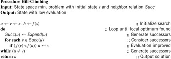
As mentioned in Chapter 6, hill-climbing selects the best successor node under some evaluation function, which we denote by f, and commits the search to it. Then the successor serves as the actual node, and the search continues. In other words, hill-climbing (for maximization problems) or gradient descent (for minimization problems) commits to changes that improve the current state until no more improvement is possible. Algorithm 14.1 assumes a state space minimization problem with objective function f to be minimized.
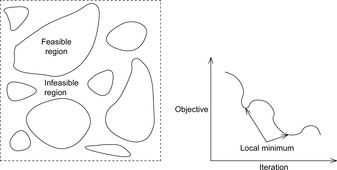
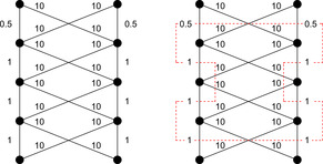
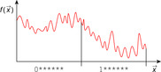
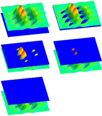
Before dropping into more general selective search strategies, we briefly reflect the main problems. The first problem is the feasibility problem. Some of the instances generated may not be valid with respect to the problem constraints: the search space divides into feasible and infeasible regions (see Fig. 14.1, left). The second problem is the optimization problem. Some greedily established local optimal solutions may not be globally optimal. In the minimization problem illustrated in Figure 14.1 (right) we have two local optima that have to be exited to eventually find the global optimum.
One option to overcome local optima is book-keeping previous optima. It may be casted as a statistical machine learning method for large-scale optimization. The approach remembers the optima of all hill-climbing applications to the given function and estimates a function of the optima. Then in stage 1 of the algorithm it uses the ending point as a starting point for hill-climbing on the estimated function of the optima. In a second stage the algorithm uses the ending point as a starting point for hill-climbing on the given function. The idea is illustrated in Figure 14.2. The oscillating function has to be minimized; known optima and the predicted optimal curve are shown. Using this function, the assumed next optima would be used as a starting state for the search.
14.3. Simulated Annealing
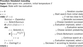
Simulated annealing is a local search approach based on the analogy of the Metropolis algorithm, which itself is a variant of randomized local search. The Metropolis algorithm generates a successor state v from u by perturbation, transferring u into v with a small random distortion (e.g., random replacement at state vector positions). If the evaluation function f, also called energy in this setting, at state v is lower than at state u then u is replaced by v, otherwise v is accepted with probability  , where k is the Boltzmann constant. The motivation is adopted from physics. According to the laws of thermodynamics the probability of an increase in energy of magnitude ΔE at temperature T is equal to
  . In fact, the Boltzmann distribution is crucial to prove that the Metropolis algorithm converges. In practice, the Boltzman constant can be safely removed or easily substituted by any other at the convenience of the designer of the algorithm. For describing simulated annealing, we expect that we are given a state space minimization problem with evaluation function f. The algorithm itself is described in Algorithm 14.2. The cooling-scheme reduces the temperature. It is quite obvious that a slow cooling implies a large increase in the time complexity of the algorithm.
The initial temperature has to be chosen large enough that all operators are allowed, as the maximal difference in cost of any two adjacent states. Cooling is often done by multiplying a constant c to T, so that the value T in iteration t equals  . An alternative is
  .
.
In the limit, we can expect convergence. It has been shown that in an undirected search space with an initial temperature T that is at least as large as the size of the minimal deterioration that is sufficient for leaving the deepest local minimum, simulated annealing converges asymptotically. The problem is that even to achieve an approximate solution we need a worst-case number of iterative steps that is quadratic in the search space, meaning that breadth-first search can perform better.
14.4. Tabu Search
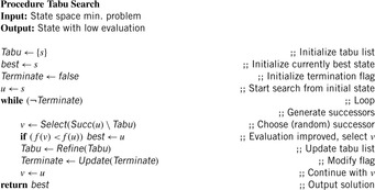
Tabu search is a local search algorithm that restricts the feasible neighborhood by neighbors that are excluded. The word tabu (or taboo ) was used by the aborigines of Tonga Island to indicate things that cannot be touched because they are sacred. In tabu search, such states are maintained in a data structure called a tabu list. They help avoid being trapped in a local optimum. If all neighbors are tabu, a move is accepted that worsen the value of the objective function to which an ordinary deepest decent method would be trapped. A refinement is the aspiration criterion: If there is a move in the tabu list that improves all previous solutions the tabu constraint is ignored. According to a provided selection criteria tabu search stores only some of the previously visited states. The pseudo code is shown in Algorithm 14.3.
One simple strategy for updating the tabu list is to forbid any state that has been visited in the last k steps. Another option is to require that local transformation does not always change the same parts of the state vector or modify the cost function during the search.
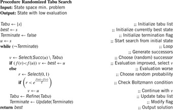
Randomized tabu search as shown in Algorithm 14.4 can be seen as a generalization to simulated annealing. It combines the reduction of the successor set by a tabu list with the selection mechanism applied in simulated annealing. Instead of the Boltzmann condition, we can accept successors according to a probability decreasing, for example, with f (u) − f (v). As with standard simulated annealing in both cases, we can prove asymptotic convergence.
14.5. Evolutionary Algorithms
Evolutionary algorithms have seen a rapid increase in their application scope due to a continuous report of solving hard combinatorial optimization problems. The implemented concepts of recombination, selection, mutation, and fitness are motivated by their similarities to natural evolution. In short, the fittest surviving individual will encode the best solution to the posed problem. The simulation of the evolutionary process refers to the genetics in living organisms on a fairly high abstraction level.
Unfortunately, most evolutionary algorithms are of domain-dependent design, while using an explicit encoding of a selection of individuals of the state space, where many exploration problems, especially in Artificial Intelligence applications like puzzle solving and action planning, are described implicitly. As we have seen, however, it is possible to encode paths for general state space problems as individuals in a genetic algorithm.
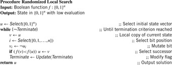
14.5.1. Randomized Local Search and (1 + 1) EA
Probably the simplest question for optimization is the following: Given  , determine the assignment to f with lowest f-value.
Randomized local search (RLS) is a variant that can be casted as an evolutionary algorithm with a population of size 1. In RLS the first state is chosen uniformly at random. Then the offspring v is obtained from u by mutation. A process called selection commits the search to successor v if its fitness f (v) is larger than or equal to f (u)(greater than or equal in the case of a minimization problem). The mutation operator of RLS as is implemented in Algorithm 14.5 chooses a position  in the state vector at random and replaces it with a different randomly chosen value. In the case of bitvectors (which is considered here), the bit is flipped. In the case of vectors from
  , one of the k − 1 different values is chosen according to the uniform distribution. RLS is a hill-climber with a small neighborhood and can get stuck in local optima. Therefore, larger neighborhoods of more local changes have been proposed.
The (1 + 1) EA also works with populations of size 1. The mutation operator changes each position independently from the others with probability 1 ∕ n. The (1 + 1) EA is implemented in Algorithm 14.6 and always finds the optimum in expected finite time, since each individual in  has a positive probability to be produced as offspring of a selected state. Although no worsening is accepted, (1 + 1) EA is not a pure hill-climber; it allows almost arbitrary big jumps.
Such search algorithms do not know if the best point ever seen is optimal. In the analysis, therefore, we consider the search as an infinite stochastic process. We are interested in the random variable at the first point of time when an optimal input is sampled. The expected value of that variable is referred to as the expected runtime.
The expected runtime and success probabilities for RLS and for the (1 + 1) EA have been studied for various functions. For example, we have the following result.
Theorem 14.1
(Expected Runtime (1 + 1) EA) For the function  the expected runtime of the (1 + 1) EA is bounded by O nlgn).
Proof
Let  . For
. For  let s (u) be the probability that mutation changes u into some
  where
where  and let
  . The expected time to leave Ai is
  , so that for a bound on the total expected runtime we have to compute
  . For our case, inputs from Ai have n + 1 − i neighbors with a larger function value. Therefore,
 Hence, the total expected runtime is bounded by

There are also families of functions for which mutation as the only genetic algorithm is provably worse than evolutionary algorithms for which a recombination operator has been defined.
14.5.2. Simple GA
Many genetic algorithms maintain a sample population of states (or their respective path generation vectors) instead of enumerating the state space state by state.
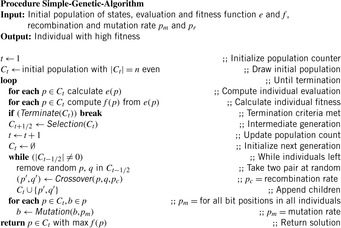
Definition 14.1
(Simple GA) A simple genetic algorithm, simple GA for short, consists of
1. The (initial) population C: A list of n individuals, n even (for proper mating).
2. The set of individuals or chromosomes  : These can be feasible and infeasible problem solutions, to be coded as a string over some alphabet Σ.
3. The evaluation function e (p): A problem depending on an object function to be minimized.
4. The fitness function f (p): A nonnegative function, derived from e (p). It correlates positively with reproduction choices φ (p) of p.
5. The selection function φ with  : A general option for the selection function is to take
  with
with  .
.
In many cases individuals are bitvectors.
Definition 14.2
(Genetic Operators) The crossover and mutation operators are defined as follows:
1. Crossover: Divide in partial sequences and recombine p′ and q′ as
• 1-point crossover:
choose random  , and set
• 2-point crossover:
choose random  , and set
• uniform crossover:
generate random bit mask  and set (bitwise Boolean operations)
2. Mutation: Each component b of a chromosome is modified with probability pm; for example,  or
or  .
.
Algorithm 14.7 depicts a general strategy for solving GAs. It is based on the four basic routines Selection, Recombination/Crossover, Mutation, and Terminate. Subsequently, to solve a problem with a genetic algorithm, we have to choose an encoding for potential solutions, choose an evaluation and a fitness function, and choose parameters n, pc, pm, and a termination criteria. The algorithm itself is then implemented, with the help of existing software libraries.
Infeasible solutions shall be sentenced by a surplus term, so that the live expectancy is small. This can be dealt with as follows. The surplus term is a function on the distance of the feasible region and the best infeasible vector is always worse than the best feasible one.
Let us consider an example. The Subset Sum problem is given by  . The feasible solutions are
  with
with  . The objective function to be maximized is
  . This problem can be reformulated as a minimization problem for the simple GA as follows:
 with fitness
  .
.
The Maximum Cut problem has a weighted graph  as input with
  and
and  for all
  . The set of feasible solutions is
  . Let
. Let  . The objective function is
  and an optimal solution C is a solution with maximal value of W (C). The encoding of V0, V1 is given by vectors
  , with
  if and only if
  . The formulation of Maximum Cut as maximizing a GA problem reads as follows:
Figure 14.3 shows an example of a cut with n = 10.
Tests with n = 100 show that after 1,000 iterations and 50,000 evaluations, obtained solutions differ from the optimum by at most 5% (on the average) with only  of the entire state space that has been looked at.
14.5.3. Insights to Genetic Algorithm Search
We now come to some insights of GAs, stating that selection and recombination is equal to innovation. Let us consider the iterated analysis of the hyperplane partition in the n-cube, the graph with nodes  , where two nodes are connected if the bit-flip (or Hamming) distance is one.
The order of  is 3 and
  . The probability that a 1-point crossover has an intersection in schema s is
  .
.
The bit-string x fits to schema s,  , if s can be changed into x by modifying at most one *. Therefore, all x that fit into s are located on a hyperplane. Every
  belongs to
  hyperplanes. There are
  different hyperplanes. A random population of size n has many chromosomes that fit to schema s of small order o (s). On the average we have
  individuals. The evaluation of x exhibits an implicit parallelism. Since x contains information of over 2n − 1 schemas, a GA senses schema, so that the representation of good schemas in the upcoming generation is increased.
Due to information loss, convergence to the optimum cannot be expected by recombination alone. We need mutation, which performs small changes to individuals and generates new information. Selection and mutation together are sufficient for performing randomized local search.
In Figure 14.4 individuals x with x1 = 0 are better than those of x1 = 1 and survive better. Therefore, the population rate in regions with  is increased.
We next try to formally quantify the changes when progressing from Ct to Ct + 1. The result, the schema theorem, is fundamental to the theory of GA. Actually, the statement is not a formal theorem but the result of some mathematical observations, important enough to be unrolled here. The schema theorem estimates a lower bound of the expected sensing rate of a schema s in going from Ct to Ct + 1.
Let the cardinality M of a schema s in iteration t be defined as  and
and  , where
The argumentation takes two conservative assumptions: each crossover is destructive, and gains are small. Then, we have where d (s, t) is the probability that a schema s is destroyed in iteration t by a crossover operation. If
  are recombined there is no loss. Let
  be the probability that of a random
  we have
  , and
, and  -.3pt. Then, insertion into (*) and division by n yields a first version of the schema theorem
By assuming that the partner of  originates in
  , we have
  Hence, the second version of the schema theorem is
 Considering the destructive effect of mutation we have
14.6. Approximate Search
To analyze the quality of a suboptimal algorithm, we take a brief excursion to the theory of approximation algorithms.
We say that algorithm A computes a c-approximation, if for all inputs I we have where mA is the value computed by the approximation and mOPT is the value computed by the optimal algorithm to solve the (maximization) problem. By this definition, the value of c is contained in [0, 1].
14.6.1. Approximating TSP
The algorithm of Christofides computes a near-optimal tour T with  , where
  is the cost of the best solution Topt. The algorithm first constructs a MST T′. Let V′ be defined as the set of vertices in T ′ with odd degree. Next it finds a minimum weight matching M on V′ (with an
  algorithm) and constructs a Euler tour T″ on the edges of
  . Lastly, it prunes shortcuts in T″ and returns the remaining tour T. The sum of degrees D of all the vertices is 2e. Therefore, D is even. If De is the sum of degrees of the vertices that have even degree, then De is also even. Therefore, D − De = 2k for some integer value k. This means that the sum of degrees of the vertices that have odd degree each is also an even number. Thus, there are even numbers of vertices having odd degree. Therefore, the minimum weighted matching on the vertices in V′ is well defined. The Euler tour based on the MST and the matching M starts and ends at the same vertex and visits all the edges exactly once. It is a complete cyclic tour, which then is truncated by using shortcuts according to the triangular property. We have
  . It remains to show that
  . Suppose that we have an optimal TSP tour To visiting only the vertices that have odd degrees. Then
  . We choose alternate edges among the edges on this path. Let M′ and M″ be two sets of edges with
  . Consequently, we have
  . Because we find the minimum matching edges M, we have
  . Combining the results, we have
  .
.
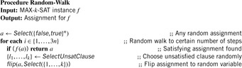
14.6.2. Approximating MAX-k-SAT
In contrast to the decision problem k-SAT with k literals in each clause, in the optimizing variant MAX-k-SAT we search for the maximal degree of satisfiability. More formally, for a formula with m clauses and n variables the task is to determine
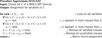
A deterministic 0.5-approximation of MAX-k-SAT is implemented in Algorithm 14.8;  denotes the simplification of a clause c with regard to assignment ai to variable xi. It is not difficult to see that the simple approximation algorithm yields an assignment that is off by at most a factor of 2. We see that for each iteration there are at least as many clauses that are satisfied as there are unsatisfied.
14.7. Randomized Search
The concept of randomization accelerates many algorithms. For example, randomized quicksort randomizes the choice of the pivot element to fool the adversary and in choosing an uneven split into two parts. Such algorithms that are always correct and that have better time performance on the average (over several runs) are called Las Vegas algorithms. For the concept of randomized search in the Monte Carlo setting, we expect the algorithm only to be m ostly c orrect (the leading characters MC used in both terms may help to memorize the classification).
In the following we will exemplify the essentials of randomized algorithms in the context of maximizing k-SAT with instances consisting of clauses of the form  . Searching for satisfying assignments for random SAT instances is close to finding a needle in a haystack. Fortunately, there is often more structure in the problem that lets heuristic value selection and assignment strategies be very effective.
The brute-force algorithm for SAT takes all 2n assignments and checks whether they satisfy the formula. The runtime is  when testing sequentially, or O (2n) when testing in the form of a binary search tree.
A simple strategy shows that there is space for improvement. Assigning the first k variables to one of the values yields a tree with 2k branches. If the k variables are chosen such that the truth value of one clause is determined, then at least one of the 2k variable assignments evaluates it to false (otherwise the clause would be trivially true for all assignments and could be omitted). Hence, at least one branch induces a backtrack and does not have to be considered further on. This implies that if the variable order is chosen along the clauses, then a backtrack approach runs in time  . Depending on the structure of the clause, in some cases, more than one branch can be pruned.
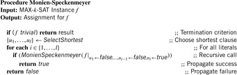
The Monien-Speckenmeyer algorithm is a deterministic k-SAT solver that includes a recursive procedure shown in Algorithm 14.9, which works on the structure of f. For k = 3 the algorithm processes the following assignments: first  , then
  , and finally
  . The recurrence relation for the algorithm is of the form
  . Assuming
  yields
  for general k and
  for k = 3 so that
  . Therefore, Monien-Speckenmeyer corresponds to an
  algorithm. With some tricks the runtime can be reduced to
  .
.
Let the probability of finding a satisfying assignment be p. The probability of not finding a satisfying assignment in t trials is  . We have
  , since
  . Therefore, the number of iterations t has to be chosen so that
  , by means
  .
.
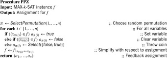
Another simple randomized algorithm for k-SAT has been suggested by Paturi, Pudlák and Zane. The iterative algorithm is shown in Algorithm 14.10. It applies one assignment at a time by selecting and setting appropriate variables, continously modifying a random seed.
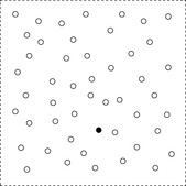
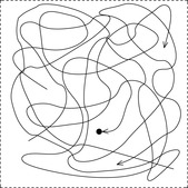
The state space to be searched is  . It is illustrated in Figure 14.5. Unsuccessful assignments are represented as hollow nodes, while a satisfying assignment is represented in the form of a black spot. The algorithm of Paturi, Pudlák, and Zane generates candidates for a MAX-k-SAT in the space.
The success probability p for one trial can be shown to be  . Subsequently, with
  iterations, we have a success probability of
  . For 3-SAT this yields an algorithm with an expected runtime of
  .
.
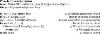
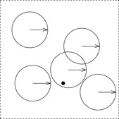
The Hamming sphere algorithm invokes a recursive procedure with parameters (a, d), where a is the current assignment and d is a depth limit. It is implemented in Algorithm 14.11 and illustrated in Figure 14.6. The initial depth value is the radius of the Hamming sphere. The spheres are illustrated as arrows in the circles denoting the spheres. Because the algorithm is called many times we have shown several such spheres, one containing a satisfying assignment.
The analysis of the algorithm is as follows. The test procedure is called t times with random  and
and  . The running time to traverse one sphere is
  . The size of the Hamming sphere of radius
  is equal to
The success probability is  . Therefore,
  iterations are needed. The running time
  is minimal for
  , such that
  .
.
Solving k-SAT with random walk works as shown in the iterative procedure of Algorithm 14.12. The algorithm starts with a random assignment and improves that by flipping the assignments to random variables in unsatisfied clauses. This procedure is closely related to the GSAT algorithm introduced in Chapter 13.
The procedure is called t times and is terminated in case of a satisfying assignment. An illustration is provided in Figure 14.7, where the walks are shown as directed curves, one ending at a satisfying assignment.
The analysis of the algorithm bases on a model of the walk in the form of a stochastic automata. It mimics the analysis of the Gambler's Ruin problem. First, we generate a binomial distribution according to the Hamming distances from the goal in a fixed assignment. Second, the transition probabilities of  (improvement toward the goal) and
  (distancing from the goal) are set. The probability to encounter the Hamming distance 0 is
14.8. Ant Algorithms
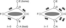
Genetic algorithms mimic biological evolution. By their success, the research in bionic algorithms that model optimization processes in nature has been intensified. Many new algorithms mimic ant search; for example, consider some natural ants while searching for food as shown in Figure 14.8. Ant communication is performed via pheromones. They trade random decision for adapted decision. In contrast to natural ants, computer ants
• solve optimizing problems via sequences of decisions;
• choose random decision, while being guided by pheromone and other criteria;
• have a limited memory;
• can detect feasible options; and
• distribute pheromones proportional to the quality of the established solution.
14.8.1. Simple Ant System
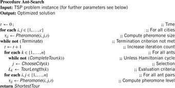
Algorithm 14.13 shows a simple ant system to find an optimized solution for the TSP problem. The parameters of the simple ant system algorithm for TSP are
1. the number of ants n. Usually we have n = c; that is, each ant starts in another city;
2. values  include the relative impact of the pheromones in relation to their visibility. If α is too big we have early stagnation or exploitation; if α is too small we have an iterative heuristic or exploration. Suggested setting: α = 1, β = 5;
3. variable ρ  influences the memory of the algorithm. If ρ is too big we have an early convergence; if ρ is too small we do not exhibit knowledge. Suggested setting: ρ = 1 ∕ 2; and
4. additional value Q that determines influence of new information in relation to initialization,  , turns out to be not crucial. Suggested setting: Q = 100.
In the algorithm we have two subroutines to be implemented.
2. Computation of pheromone size  for (i, j):
If t = 0 then  is newly initialized, otherwise a fraction (1 − ρ) disappears and ant k distributes
  :
:
Tests show that the algorithm is successful with parameters (α = 1, β = 1, ρ = 0.9, Q = 1,  ).
).
14.8.2. Algorithm Flood
Another important option for optimization is simulated annealing. Since we are only interested in the main characteristic of this technique we prefer the interpretation as a form of ant search. Suppose ants are walking on a landscape that is slowly flooded by water as shown in Figure 14.9. The hope is that at the end an ant will be positioned on the highest mountain corresponding to the best evaluation possible.
In the pseudo-code presentation in Algorithm 14.14 each ant has a position (initialized with SelectPosition) and its position corresponds to a solution of the problem. There are neighbors' positions in Succ that can be reached by applying operators. The quality of the solution is measured by the evaluation function height. The water level level is a slowly rising parameter and the call to Dry indicates that only dry ants remain active. Tests show the effectiveness of the algorithm for problems with many neighbors.
As in the case of GAs, algorithm flood can be easily adapted to general heuristic search state space problems by using ants' encodings for paths, a suitable neighborhood relation, and the heuristic estimate as the evaluation function.
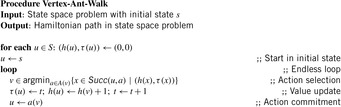
14.8.3. Vertex Ant Walk
A real-time search variant, often mentioned together with ant algorithms, is vertex ant walk. It is defined by the rules in Algorithm 14.15 and has no explicit termination criterion.

A tie can only occur between yet unvisited states. Once a state is visited, it always has a unique time stamp that avoids further ties.
Theorem 14.2
(Properties VAW)Algorithm 14.15fulfills the following properties:
1. For (u, v) as an edge in the state space problem graph G = (V, E), it always holds that  .
.
2. Let t be the t-th iteration and  be the h-value in iteration t. At all times t, we have
  .
.
3. A single ant covers any connected graph within O (nd) steps, where n is the number of vertices and d is the diameter of the graph.
4. A Hamiltonian cycle, upon being traversed n consecutive times, becomes a limit cycle of VAW.
Proof
2. Denote the sequence of nodes visited up to time t by  , and the h-value of a vertex u upon completion of time step t by
  . The only change to h may occur at the vertex currently visited, hence
  , where Δi is the offset to h (G) at time i,
  . According to the VAW rule, upon moving from ui to
  the value of
  is set to
  and
and  . Together with
  by substituting i = t − 1 we have
  . Recursively applying the analysis, we have
 Since
Since  we finally get
  . The result follows by the rules
  and
and  .
.
3. We shall prove a slightly stronger claim: After at most  steps the graph is covered. Assume the contrary. Then there is at least one node, say u, for which h (u) = 0. According to the first lemma none of u's neighbors can have
  and none of u's neighbors' neighbors can have
  , and so on. Therefore, we have at least one node with h = 0, at least one node with h = 1, and so on up to d − 1. For the rest of the at most n − d nodes we have
  . This yields
  . According to the second lemma, the total value of h at time t is at least t, so that after at most
  steps the graph is covered.
4. If the graph has a Hamiltonian cycle, following this cycle is clearly the shortest way to cover the graph. Recall that a closed path in a graph is a Hamiltonian cycle if it visits each node exactly once. We shall see that a Hamiltonian cycle is a possible limit of VAW. Moreover, if the ant happens to follow the cycle for n consecutive times, it will follow this cycle forever.
Recall that upon leaving a node u, we have  . Let us now assume that at time t the ant has completed a sequence of n Hamiltonian cycles. Then
  has not been visited since time t − n + 1 and
  . Substituting the first equation into the second yields
 During the (n + 1) st cycle, the ant is confronted with the same relative h pattern with which it was confronted in the first cycle. The value n that is added to each h value does not change the ordering relation between the nodes. Therefore, the same decisions are taken.
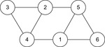
The bound of O (nd) is tight. There are examples of graphs, where the cover time is indeed O (nd). Consider a graph that consists of triangles that are connected in a single chain, with one additional node between the triangles (see Fig. 14.10). It is easy to validate that the triangles are in fact traps for VAW that cause the ant to go back to its starting point. There are n vertices, and the diameter is about 0.8n. The time needed to traverse the graph is  .
.
The last results hold for a single ant. They are not in general true for multiple ants, but it seems reasonable to say that if the graph is large and the ants are fairly distributed in the beginning, the load will be more or less balanced. In edge ant walk (EAW) edges rather than nodes are marked. For this process it can be shown that k small-oriented ants can cover a graph in at most  steps, where δ is the maximum vertex-degree and n is the number of nodes. In practice, VAW often performs better than edge ant walk, since in general,
  .
.
14.9. * Lagrange Multipliers
In continuous nonlinear programming (CNLP), we have continuous and differential functions f,  , and
, and  . The nonlinear program Pc given as
 subject to
 is to be solved by finding a constrained local minimum x with respect to the continuous neighborhood
  of x for some ϵ > 0. A point x* is a constraint local minimum (CLM) if x* is feasible and
  for all feasible
  .
.
Based on Lagrange-multiplier vectors  and
and  , the Lagrangian function of Pc is defined as
14.9.1. Saddle-Point Conditions
A sufficient saddle-point condition for x * in Pc is established if there exist λ* and μ* such that for all x satisfying
  and all
  and
and  . To illustrate that the condition is only sufficient, consider the following CLNP:
 It is obvious that x* = 5 is a CLM. Differentiating the Lagrangian
  with respect to x and evaluating it at x* = 5 yields
  , which implies λ* = 10. However, since the second derivative is
  , we know that L (x, λ) is at a local maximum at x* instead of a local minimum. Hence, there exists no λ* that satisfies the sufficient saddle-point condition.
To devise a sufficient and necessary saddle-point condition we take the transformed Lagrangian for Pc defined as where
where  is defined as
  and
and  is given by
  .
.
A point  is regular with respect to the constraints, if the gradient vectors of the constraints are linearly independent.
Theorem 14.3
(Extended Saddle-Point Condition) Suppose  is regular. Then x* is a CLM of, Pc if and only if there exist finite
  and
and  such that, for any
  and
and  , the following condition is satisfied:
Proof
The proof consists of two parts. First, given x*, we need to prove that there exist finite  and
and  that satisfy the preceding condition. The inequality on the left side is true for all α and β because x* is a CLM, which implies that
  and
and  .
.
To prove the inequality on the right side, we know that the gradient vectors of the equality and the active inequality constraints at x* are linear-independent, because x* is a regular point. According to the necessary condition on the existence of a CLM by Karush, Kuhn, and Tucker (see Bibliographic Notes) there exist unique λ* and μ* that satisfy  , where
  and
and  if
if  . When we divide the index sets for h and g into negative and nonnegative sets, we get
• 
• 
• 
• 
Differentiating the Lagrangian function  with respect to x yields
Assuming  and
and  and
and  we evaluate
  for all
  and
and  as follows:
Assuming  and using a Taylor series expansion of the functions around x/ we have
Since
• for all 
• for all 
• for all 
• for all 
The second part of the proof assumes that the condition is satisfied, and we need to show that x* is a CLM. Point x* is feasible because the inequality on the left side can only be satisfied when  and
and  . Since
  and
and  , the inequality of the right side ensures that x* is a local minimum when compared to all feasible points in
  . Therefore, x* is a CLM.
The theorem requires  and
and  instead of
  and
and  because Lc may not be a strict local minimum when
  and
and  . Consider the example CNLP with
  . At the only CLM
  ,
,  is not a strict local minimum when
  , but when
  .
.
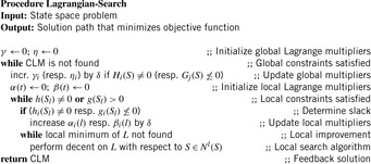
The algorithmic solution according to the theorem is iterative in nature with the pseudo code given in Algorithm 14.16.
Theorem 14.3 transfers to discrete and mixed (continuous and discrete) state spaces. The difference in discrete (mixed) space is the definition discrete (mixed) neighborhood Nd (N m). Intuitively, Nd represents points that can be reached from y in one step, regardless whether there is a valid action to effect the transition. We require  if and only if
  ). A mixed neighborhood
  of a point x in continuous space and a point y in discrete space can be defined as

14.9.2. Partitioned Problems
The goal of solving state space problems can be reduced to the previous setting. Our formulation assumes that the (possibly continuous) time horizon is partitioned in k + 1 stages, with ul local variables, ml local equality constraints, and rl local inequality constraints in stage l,  .
.
Such partitioning decomposes the state variable vector S of the problem into k + 1 subvectors  , where
  is a ul-element state vector in (mixed) state space at stage l, and Si(l) is the i th dynamic state variable in stage l. Usually ut is fixed. A solution to such a problem is a path that consists of the assignments of all variables in S. A state space search problem can be written as
  subject to
  ,
,  ,
,  (the local constraints ), and H (S) = 0,
  (the global constraints ). Here, hl and gl are vectors of local-constraint functions that involve Sl and time in stage t; and H and G are vectors of global-constraint functions that involve state variables and time in two or more stages.
We define the neighborhood of a solution path  as follows. The partitionable (mixed) neighborhood of a path p is defined as
 where N (pl) is the state space neighborhood of state vector Sl in stage l. Intuitively, N (p) is partitioned into k + 1 disjoint sets of neighborhoods, each perturbing one of the stages.
Here N (p) includes all paths that are identical to S in all stages except l, where S (l) is perturbed to a neighboring state in  . For example, let
  for each stage in a three-stage problem and p = (2, 2, 2). Then N (p) is given by
  ,
,  , and
, and  ; that is, the union of the perturbation of p in stages 1, 2, and 3.
Algorithm 14.17 gives the iterative algorithm for computing an optimal solution. For a fixed γ and ν the program finds Sl that solves the following mixed-integer linear program in stage l:  subject to
  and
and  . As a result, the solution of the original problem is now reduced to solving multiple smaller subproblems of which the solutions are collectively necessary for the final solution. Therefore, the approach reduces significantly the efforts in finding a solution, since the size of each partition will lead to a reduction of the base of the exponential complexity when a problem is partitioned.
The entire Lagrangian function that is minimized is
As in Theorem 14.3, necessary and sufficient conditions for L can be established, showing that algorithm Lagrangian Search will terminate with an optimal solution.
14.10. * No-Free-Lunch
Despite all successes in problem solving, it is clear that a general problem solver which solves all optimization problems is not to be expected. With their no-free-lunch theorems, Wolpert and Macready have shown that any search strategy performs exactly the same when averaged over all possible cost functions. If some algorithm outperforms another on some cost function, then the latter one must outperform the former one on others. A universally best algorithm does not exist. Even random searchers will perform the same on average on all possible search spaces. Other no-free-lunch theorems show that even learning does not help. Consequently, there is no universal search heuristic. However, there is some hope. By considering specific domain classes of practical interest, the knowledge of these domains can certainly increase performance. Loosely speaking, we trade the efficiency gain in the selected problem classes with the loss in other classes. The knowledge we encode in search heuristics reflects state space properties that can be exploited.
A good advice for a programmer is to learn different state space search techniques and understand the problem to be solved. The ability to devise effective and efficient search algorithms and heuristics in new situations is a skill that separates the master programmer from the moderate one. The best way to develop that skill is to solve problems.
14.11. Summary
In this chapter, we studied search methods that are not necessarily complete but often find solutions of high quality fast. We did this in the context of solving optimization problems in general and used, for example, traveling salesperson problems as examples. Many of these search methods then also apply to path planning problems, for example, by ordering the actions available in states and then encoding paths as sequences of action indices.
The no-free-lunch theorems show that a universally best-search algorithm does not exist since they all perform the same when averaged over all possible cost functions. Thus, search algorithms need to be specific to individual classes of search problems.
Complete search methods are able to find solutions with maximal quality. Approximate search methods utilize the structure of search problems to find solutions of which the quality is only a certain factor away from maximal. Approximate search methods are only known for a small number of search problems. More general search methods typically cannot make such guarantees. They typically use hill-climbing (local search) to improve an initial random solution repeatedly until it can no longer be improved, a process that is often used in nature, such as in evolution or for path finding by ants. They often find solutions of high quality fast but do not know how good their solutions are.
To use search methods based on hill-climbing, we need to carefully define which solutions are neighbors of a given solution, since search methods based on hill-climbing always move from the current solution to a neighboring solution. The main problem of search methods based on hill-climbing are local maxima since they cannot improve the current solution any longer once they are at a local maximum. Thus, they use a variety of techniques to soften the problem of local maxima. For example, random restarts allow search methods based on hill-climbing to find several solutions and return the one with the highest quality. Randomization allows search methods based on hill-climbing to be less greedy yet simple, for example, by moving to any neighboring solution of the current solution that increases the quality of the current solution rather than only the neighboring solution that increases the quality of the current solution the most. Simulated annealing allows search methods based on hill-climbing to move to a neighboring solution of the current solution that decreases the quality. The probability of making such a move is larger the less the quality decreases and the sooner the move is made. Tabu search allows search methods based on hill-climbing to avoid previous solutions. Genetic algorithms allow search methods based on hill-climbing to combine parts of two solutions (recombinations) and to perturb them (mutations).
Although most of the chapter was dedicated to discrete search problems, we also showed how hill-climbing applies to continuous search problems in the context of hill-climbing for continuous nonlinear programming.
In Table 14.1 we have summarized the selective search strategies as proposed in this chapter. All algorithms find local optimum solutions, but in some cases arguments are given for why the local optimum should not be far off from the global optimum. In this case we wrote Global together with a star denoting that this will be achieved only in the theoretical limit, not in practice. We give some hints on the nature of theoretical analyses behind it, and the main principle that is simulated to overcome the state explosion problem.
| Algorithm | Optimum | Neighbors | Principle |
|---|---|---|---|
| Simulated annealing (14.2) | Global* | General | Temperature |
| Tabu (14.3) | Local | General | Forced cuts |
| Randomized tabu (14.4) | Local | General | Forced/random cuts |
| Randomized local search (14.5) | Local | Boolean | Selective/mutation |
| (1 + 1) GA (14.6) | Global* | Boolean | Selective/mutation |
| Simple GA (14.7) | Global* | General | Selective/mutation/recombination |
| Vertex Ant search (14.15) | Cover | Specific | Pheromones |
| Ant search (14.13) | Global* | Specific | Pheromones |
| Flood (14.14) | Local | General | Water level |
| Lagrangian (14.16, 14.17) | CLM | MIXED | Multipliers |
Table 14.2 summarizes the results of randomized search in k-SAT problems, showing the base α in the runtime complexity of  . We see that for larger values of k the values converge to 2. In fact, compared to the naive
  algorithm with base α = 2, there is no effective strategy with better α in general SAT problems.
14.12. Exercises
14.1 Validate empirically that the phase transition for 3-SAT is located at  by randomly generating 3-SAT formulas and running an SAT solver.
14.2 In this exercise we develop a randomized (3/4)-approximation of MAX-2-SAT.
1. Give a randomized  -approximation (RA) that simply selects a random assignment. Given clauses C of length k show that the probability that clause C is satisfied is
  .
.
2. Illustrate the working of randomized rounding (RR) where an SAT formula is substituted by a linear program (LP), for example, clause  is converted to
 Then the solutions are computed with an efficient LP solver. The solutions are taken as probabilities to draw Boolean values for the assignment variables.
3. Show that the combined run of RA and RR yields a (3/4)-approximation for MAX-2-SAT. Instead of proving the theorem formally, you may work out a small example.
14.3 As another example for a randomized algorithm we chose the probabilistic reduction of three-dimensional matching (3-DM) on 2-SAT. The idea is as follows. With probability of 1/3 one of the colors in  is omitted. The resulting problem is converted into a 2-SAT instance with variables
  (v for the node and j for the color). The clauses are of the form
  and
and  .
.
1. Show that the probability of the correct choice of colors is  .
.
2. Show that we need  iterations for a running time of
  .
.
3. Using this reduction principle to show that a CSP with binary constraints (the domain of each variable is D) is solvable in time  .
.
14.4 Most k-SAT solvers can be extended to constraint satisfaction problems (CSP), where k is the order of the constraints and assignments. For the sake of simplicity assume that the domains of all variables are the same (D).
1. For Hamming sphere infer a runtime of  .
.
2. For random walk establish a runtime of  . Show that for k = 2, this bound for random walk matches the one obtained for reduction in the previous exercise.
14.5 The algorithm of Monien-Speckenmeyer has been improved by using autarkic assignments. An assignment b is called autarkic for f, if all clauses, with at least one b variable, are already satisfied. For example, the assignment b = (0, 0) is autarkic for  , since only the first two clauses contain x1 and x2, and these clauses are set to 1 by b.
1. Give another autarkic assignment for f.
2. Describe the changes to the algorithm of Monien and Speckenmeyer to include autarkic assignments.
14.6 Change the order of Ws and Bs in _WWWBBB to WWWBBB_. You are allowed to jump over at most two places provided that the target location is free. It is not required that the empty place is in the front.
1. Determine an optimal solution by hand.
2. Use an evaluation function that counts the number of Bs to the left of each W, summed over all three Ws. Apply genetic heuristic search to find a solution.
14.7 Consider Simple-GA on the fitness function  , with
  by using a binary string encoding of the two individuals p = 1 and q = 10.
1. Determine the maximum of the function analytically.
2. Does the algorithm arrive at the optimum using bit mutation and 1-point crossover, both with regard to random bit positions?
14.8 Implement and run genetic heuristic search to the same instance. Use 100 randomly generated paths of length 65 to start with and apply 1,000 iterations of the algorithm.
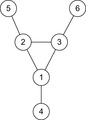
14.10 Perform VAW on the graph of Figure 14.11.
1. Denote the tuples  ,
,  starting at node 1.
2. When is the graph completely covered?
3. How long is the limit cycle?
4. Denote the node sequence in the final tour as a regular expression.
5. Is the limit cycle Hamiltonian?
14.11 Perform VAW on the graph of Figure 14.12.
1. Denote the tuples  ,
,  starting at node 1.
2. When is the graph completely covered?
3. How long is the limit cycle?
4. Denote the node sequence in the final tour as a regular expression.
5. Is the limit cycle Hamiltonian?
14.13 For algorithm Flood take function  to be optimized, with respect to a 10 × 10 grid. Start with n = 20 active ants at random position. Initialize W to 0 and increase it by 0.1 for each iteration.
14.14 Express the previous exercises now with real values on  as a continuous nonlinear programming task.
1. What is the constraint local minimum (CLM) for this function?
2. Express the optimization problem with Lagrangian multipliers.
3. Is it the global optimum?
14.15 Heuristics for discrete domains are often found by relaxation of the problem formulation from an integer program to a linear program.
1. Formulate Knapsack as a (0/1) integer program.
2. Relax the integrality constraints to derive an upper bound on Knapsack.
14.16 In the Ladder problem a ladder leans across a five-foot fence, just touching a high wall three feet behind the fence.
1. What is the minimum possible length l of the ladder? Use standard calculus. Hint: The formula  describes a circle with center (−3, −5) and radius L. The proportionality of base and height for the two smaller right triangles yields ab = 15. Substitute this in the first equation to obtain the single-variable function.
2. Provide the objective function F (a, b) with constraint function G (a, b) = 0 and solve the problem using Lagrange multipliers to find a set of three equations in three unknowns.
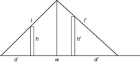
14.17 Consider now the Two Ladder problem with two ladders of lengths l and l′ leaning across two walls of given heights h = 10 and h′ = 15 bordering a gap of given width W = 50 (see Fig. 14.13). The lower ends of the ladders are placed at distances d′ and d′ from the walls, so that their upper ends meet at a point above the water. The two ladders are supported in place by each other as well as by the two walls. The problem is to find this minimal sum of l and l′.
1. Model and solve the problem by ordinary calculus.
2. Model and solve the problem as a Lagrange optimization problem.
14.13. Bibliographic Notes
Hill-climbing and gradient decent algorithms belong to the folklore of computer science. Algorithm flood is a version of simulated annealing, which has been introduced by Kirkpatrick, Jr., and Vecchi (1983). Randomized tabu search appeared in Faigle and Kern (1992). Annealing applies to optimization problems where direct methods are trapped; while simulated tempering, for example, by Marinari and Parisi (1992) and swapping by Zheng (1999) are applied when direct methods perform poorly. The standard approach for sampling via Markov chain Monte Carlo from nonuniform distributions is the Metropolis algorithm (Metropolis, Rosenbluth, Rosenbluth, Teller, and Teller, 1953). There is a nice discussion about lifting space and solution state spaces in the beginning by Hoos and Stützle (2004).
Ant walk generalized the use of diminishing pebbles by a model of odor markings. Vertex ant walk has been introduced by Wagner, Lindenbaum, and Bruckstein (1998). It is a reasonable trade-off between sensitive DFS and self-avoiding walk by Madras and Slade (1993). Edge ant walk has been proposed by Wagner, Lindenbaum, and Bruckstein (1996). Thrun (1992) has described counterbased exploration methods, which is similar to VAW, but the upper bound shown there on the cover time is  , where d is the diameter and n is the number of vertices.
Satisfiability problems have been referenced in the previous chapter. Known approximation ratios for MAX-SAT are 0.7846; MAX-3-SAT, 7/8, upper bound 7/8; MAX-2-SAT, 0.941, upper bound 21/22=0.954; MAX-2-SAT with additional cardinality constraints, 0.75; see Hofmeister (2003). Many inapproximability results are based on the PCP theory, denoting that the class of NP is equal to a certain class of probabilistically checkable proofs (PCP). For example, this theory implies that there is an ϵ > 0, so that it is NP-hard to find an (1 − ϵ) approximation for MAX-3-SAT. PCP theory has been introduced by Arora (1995). The technical report based on the author's PhD thesis contains the complete proof of the PCP theorem, and basic relations to approximation algorithms.
The algorithms of Monien and Speckenmeyer (1985) and of Paturi, Pudlák, and Zane (1977) have been improved by the analysis of Schöning (2002), who has also studied random walk and Hamming sphere as presented in the text. Hofmeister, Schöning, Schuler, and Watanabe (2002) have improved the runtime of a randomized solution to 3-SAT to  , and Baumer and Schuler (2003) have further reduced it to
  . A deterministic algorithm with a performance bound of
  has been suggested by Dantsin, Goerdt, Hirsch, and Schöning (2000). The
  lower-bound result of Miltersen, Radhakrishnan, and Wegener (2005) shows that a conversion of conjunctive normal for (CNF) to disjunctive normal form (DNF) is almost exponential. This suggest that
  algorithms for general SAT with
  are not immediate.
Genetic algorithms are of widespread use with their own community and conferences. Initial work on genetic programming including the Schema Theorem has been presented by Holland (1975). A broad survey has been established in the triology byKoza (1992) and Koza (1994) and Koza, Bennett, Andre, and Keane (1999). Schwefel (1995) has applied evolutionary algorithms to optimize airplane turbines. Genetic path search has been introduced in the context of model checking by Godefroid and Khurshid (2004).
Ant algorithms also span a broad community with their own conferences. A good starting point is the special issue on Ant Algorithms and Swarm Intelligence by Dorigo, Gambardella, Middendorf, and Stützle (2002) and a book by Dorigo and Stützle (2004). The ant algorithm for TSP is due to Gambardella and Dorigo (1996). It has been generalized by Dorigo, Maniezzo, and Colorni (1996).
There is a rising interest in (particle) swarm optimization algorithms (PSO), a population-based stochastic optimization technique that originally has been developed by Kennedy and Eberhart. It closely relates to genetic algorithms with different recombination and mutation operators (Kennedy, Eberhart, and Shi, 2001). Applications include time-tabling as considered by Chu, Chen, and Ho (2006), or stuff scheduling as studied by Günther and Nissen (2010). Mathematical programming has a long tradition with a broad spectrum of existing techniques especially for continuous and mixed-integer optimization. The book Nonlinear Programming by Avriel (1976) provides a good starting point. For CNLP, Karush, Kuhn, and Tucker (see Bertsekas (1999)) have given another necessary condition. If only equality constraints are present in Pc, we have n + m equations with n + m unknowns (x, λ) to be solved by iterative approaches like Newton's method. A static penalty approach transforms Pc into the unconstraint problem  very similar to the one considered in the text (set ρ = 1). However, the algorithm may be hard to carry out in practice because the global optimum of Lρ needs to hold for all points in the search space, making α and β very large.
Mixed-integer NLP methods generally decompose MINLP into subproblems in such a way that after fixing a subset of the variables, each resulting subproblem is convex and easily solvable, or can be relaxed and approximated. There are four main types: generalized Benders decomposition by Geoffrion (1972), outer approximation by Duran and Grossmann (1986), generalized cross-decomposition by Holmberg (1990) and branch and reduce methods by Ryoo and Sahinidis (1996).
There is some notion of completeness for selective algorithms called probabilistic approximate completeness (PAC) (Hoos and Stützle (1999), (Hoos and Stützle, 1999). Randomized algorithms, which are not PAC, are essentially incomplete. The intuition is that if the algorithm is left to run infinitely, a PAC algorithm will almost certainly find a solution, if it exists. In other words, algorithms that are PAC can never get trapped in nonsolution regions of the search space. However, they may still require a very long time to escape from such regions; see, for example, Hoos and Stützle (2004). Whether this theoretical property has practical impact is uncertain. This may change, if combined with results on the failure probability's rate of convergence.
The first no-free-lunch theorems have been given by Wolpert and Macready (1996). Culberson (1998b) has given an algorithmic view of no-free-lunch. More recent results on the NFL theory have been established by Droste, Jansen, and Wegener (1999) and Droste, Jansen, and Wegener (2002).
..................Content has been hidden....................
You can't read the all page of ebook, please click here login for view all page.