
Chapter 1. Introduction
This chapter introduces notational background, specific puzzles, and general problem formalisms. It recalls the success story of heuristic search and studies heuristics as efficiently computable lower bounds.
Keywords: computability theory, complexity theory, asymptotic resource consumption, symbolic logic, traveling salesman problem, sliding-tile problem, Sokoban, Rubik's Cube, route planning, STRIPS-type planning, production system, Markov decision process, consistent heuristic, admissible heuristic
In this book, we study the theory and the applications of heuristic search algorithms. The general model is the guided exploration in a space of states.
After providing some mathematical and notational background and motivating the impact of search algorithms by reflecting several success stories, we introduce different state space formalisms. Next we provide examples of single-agent puzzles such as the (n2 − 1)-Puzzle and extensions to it, the Rubik's Cube, as well as Sokoban problems. Furthermore, the practically important application areas of Route Planning and Multiple Sequence Alignment are introduced. The former is fundamental to vehicle navigation and the latter is fundamental to computational biology. In the TSP we consider the computation of round trips. For each of the domains, we introduce heuristic evaluation functions as a means to accelerate the search. We motivate them graphically and formalize them. We define properties of heuristics, such as consistency and admissibility, and how they are related. Moreover, we define the general descriptive schemes of production systems, Markov decision process problems, and action planning. For the case of a production system, we will see that general state space problem solving is in fact undecidable. For the case of action planning, we will see how to derive some problem-independent heuristics.
1.1. Notational and Mathematical Background
Algorithms are specifications of action sequences, similar to recipes for cooking. The description should be concrete enough to cook a tasteful meal. On the other hand, some abstraction is necessary to keep the presentation readable; we don't teach the cook how to dice onions. In presenting algorithms in computer science, the situation is similar. The presentation should be concrete enough to allow analysis and reimplementation, but abstract enough to be ported on different programming languages and machines.
1.1.1. Pseudo Code
A program representation in a fictitious, partly abstract programming language is called pseudo code. However, its intention is to give a high-level description of an algorithm to a human, not to a machine. Therefore, irrelevant details (e.g., memory management code) are usually omitted, and sometimes natural language is used when convenient.
Most programs consist of assignments (←), selection (e.g., branching based on if conditions), and iteration (e.g., while loops). Subroutine calls are important to structure the program and to implement recursion, and are shown in italics. In the pseudo code implementations, we use the following constructs.
if (〈condition〉) 〈body 〉else 〈alternative〉
Branching of the program based on the case selected in the Boolean predicate condition.
and, or, not
Logical operation on Boolean conditions.
while (〈condition〉) 〈body〉
Loop to be checked prior to the execution of its body.
do 〈body 〉while (〈condition〉)
Loop to be checked after the execution of its body.
for each 〈element 〉in 〈Set〉
Variable element iterates on the (often ordered) set Set.
return
Backtrack to calling procedure with result.
Conditional and loop constructs introduce compound statements; that is, the parts of the statements constitute lists of statements (blocks) themselves. To clarify the hierarchical structure of the program, sometimes explicit begin and end statements are given. Different from this convention, in this book, in the interest of succinctness we chose to rely solely on indentation. For example, in the following fragment, note the end of the block that is executed in case the condition evaluates to false:
if (〈condition〉)
〈if-true-statement 1〉
〈if-true-statement 2〉
…
else
〈if-false-statement 1〉
〈if-false-statement 2〉
…
〈after-if-statement 1〉
…
For easier understanding, each line in the pseudo code is annotated with some short comments, separated from the program code by a double semicolon.
1.1.2. Computability Theory
Computability theory is the branch of theoretical computer science that studies which problems are computationally solvable using different computation models. Computability theory differs from the related discipline of computational complexity theory (see next section) in asking whether a problem can be solved at all, given any finite but arbitrarily large amount of resources.
A common model of computation is based on an abstract machine, the Turing machine (see Fig. 1.1). The computational model is very simple and assumes a computer M in the form of a 7-tuple  , with state set Q, input alphabet Σ, tape alphabet Γ, transition function
  , blank symbol B, final state set F, and head position q0.

The machine takes some input word  over the alphabet Σ and assumes that it is already located on the tape at position
  . The initial head position is 1. The process of computation terminates, if some final state in F is reached. The state transition function δ sets the new state in Q, which can be interpreted as performing on step in the program that is run on the Turing machine. Then a character is written on the tape at the current head position. Depending on the value in
  the head is moved to the left (L), to the right (R), or remains unchanged (N), respectively. The output of the computation is the content of the tape after termination. The machine solves a decision problem when for an input string, it produces a binary output signifying “yes” or “no.” A problem is decidable if a Turing machine exists that always gives an answer in finite time.
Since the time of Turing, many other formalisms for describing effective computability have been proposed, including recursive functions, the lambda calculus, register machines, Post systems, combinatorial logic, and Markov algorithms. The computational equivalence of all these systems corroborates the validity of the Church-Turing thesis: Every function that would naturally be regarded as computable can be computed by a Turing machine.
A recursively enumerable set S is a set such that a Turing machine exists that successively outputs all of its members. An equivalent condition is that we can specify an algorithm that always terminates and answers “yes” if the input is in S; if the input is not in S, computation might not halt at all. Therefore, recursively enumerable sets are also called semi-decidable.
A function f(x) is computable if the set of all input–output pairs is recursively enumerable. Decision problems are often considered because an arbitrary problem can always be reduced to a decision problem, by enumerating possible pairs of domain and range elements and asking, “Is this the correct output?”
1.1.3. Complexity Theory
Complexity theory is part of the theory of computation dealing with the resources required during computation to solve a given problem, predominantly time (how many steps it takes to solve a problem) and space (how much memory it takes). Complexity theory differs from computability theory, which deals with whether a problem can be solved at all, regardless of the resources required.
The class of algorithms that need space s(n), for some function s(n), is denoted by the class DSPACE(s(n)); and those that use time t(n) is denoted by DTIME(t(n)). The problem class P consists of all problems that can be solved in polynomial time; that is, it is the union of complexity classes DTIME(t(n)), for all polynomials t(n).
A nondeterministic Turing machine is a (nonrealizable) generalization of the standard deterministic Turing machine of which the transition rules can allow more than one successor configuration, and all these alternatives can be explored in parallel (another way of thinking of this is by means of an oracle suggesting the correct branches). The corresponding complexity classes for nondeterministic Turing machines are called NSPACE(s(n)) and NTIME(s(n)). The complexity class NP (for nondeterministic polynomial) is the union of classes NTIME(t(n)), for all polynomials t(n). Note that a deterministic Turing machine might not be able to compute the solution for a problem in NP in polynomial time, however, it can verify it efficiently if it is given enough information (a.k.a. certificate) about the solution (besides the answer “yes” or “no”).
Both P and NP are contained in the class PSPACE, which is the union of DSPACE(s(n)) for any polynomial function s(n); PSPACE doesn't impose any restriction on the required time.
A problem S is hard for a class  if all other problems
  are polynomially reducible to C; this means that there is a polynomial algorithm to transform the input x′ of S′ to an input x to S, such that the answer for S applied to x is “yes” if and only if the answer for S′ applied to x′ is “yes.” A problem S is complete for a class
  if it is a member of
  and it is hard for
  .
.
One of the big challenges in computer science is to prove that P ≠ NP. To refute this conjecture, it would suffice to devise a deterministic polynomial algorithm for some NP-complete problem. However, most people believe that this is not possible. Figure 1.2 graphically depicts the relations between the mentioned complexity classes.

Although the model of a Turing machine seems quite restrictive, other, more realistic models, such as random access machines, can be simulated with polynomial overhead. Therefore, for merely deciding if an algorithm is efficient or not (i.e., it inherits at most a polynomial time or at least an exponential time algorithm), complexity classes based on Turing machines are sufficiently expressive. Only when considering hierarchical and parallel algorithms will we encounter situations where this model is no longer adequate.
1.1.4. Asymptotic Resource Consumption
In the previous section, we had a quite crude view on complexity classes, distinguishing merely between polynomial and more than polynomial complexity. While the actual degree of the polynomial can be preeminently important for practical applications (a “polynomial” algorithm might still not be practically feasible), exponential complexity cannot be deemed efficient because multiple resources are needed to increase the input size.
Suppose the two functions  and
and  describe the time or space used by two different algorithms for an input of size n. How do we determine which algorithm to use? Although f2 is certainly better for small n, for large inputs its complexity will increase much more quickly. The constant factors depend only on the particular machine used, the programming language, and such, whereas the order of growth will be transferable.
The big-oh notation aims at capturing this asymptotic behavior. If we can find a bound c for the ratio  , we write
  . More precisely, the expression
  is defined that there exist two constants n0 and c such that for all
  we have
  . With the previous example we could say that
  and
and  .
.
The little-oh notation constitutes an even stricter condition: If the ratio approaches zero in the limit, we write  . The formal condition is that there exists an n0 such that for all
  , we have
  , for each
  . Analogously, we can define lower bounds:
  and
and  , by changing the ≤ in the definition by ≥, and < by >. Finally, we have
  if both
  and
and  hold.
hold.
Some common complexity classes are constant complexity (O(1)), logarithmic complexity (O(lgn)), linear complexity (O(n)), polynomial complexity (O(nk), for some fixed value of k and exponential complexity (e.g., O(2n)).
For refined analysis we briefly review the basics on amortized complexity. The main idea is to pay more for cheaper operations and use the savings to cover the more expensive ones. Amortized complexity analysis distinguishes between tl, the real cost for operation l; Φl, the potential after execution operation l; and al, the amortized costs for operation l. We have  and
and  ,
, and
and so that the sum of the real costs can be bounded by the sum of the amortized costs.
To ease the representation of the exponential algorithms, we abstract from polynomial factors. For two polynomials p and q and any constant  , we have that
  . Therefore, we introduce the following notation:
1.1.5. Symbolic Logic
Formal logic is a powerful and universal representation formalism in computer science, and also in this book we cannot completely get around it. Propositional logic is defined over a domain of discourse of allowed predicate symbols, P. An atom is an occurrence of a predicate. A literal is either an atom p or the negation of an atom, ¬p. A propositional formula is recursively defined as an atom or a compound formula, obtained from connecting simpler formulas using the connectives ∧(and), ∨(or), ¬(not), →(if-then), ⇔(equivalent), and ⊕(exclusive-or).
While the syntax governs the construction of well-formed formulas, the semantics determine their meaning. An interpretation maps each atom to either true or false (sometimes these values are given as 0 and 1). Atoms can be associated with propositional statements such as “the sun is shining.” In compositional logic, the truth of a compound formula is completely determined by its components and its connectors. The following truth table specifies the relations. For example, if p is true in an interpretation I, and q is false, then  is false in I.
| p | q | ¬p | |||||
| 0 | 0 | 0 | 0 | 0 | 1 | 1 | 0 |
| 0 | 1 | 0 | 0 | 1 | 1 | 0 | 1 |
| 1 | 0 | 1 | 0 | 1 | 0 | 0 | 1 |
| 1 | 1 | 1 | 1 | 1 | 1 | 1 | 0 |
A propositional formula F is satisfiable or consistent if it is true in some interpretation I; in this case, I is called a model of F. It is a tautology (or valid) if it is true in every interpretation (e.g.,  ). A formula G is implied by F if G is true in all models of F.
Propositional formulas can always be equivalently rewritten either in disjunctive normal form (i.e., as a disjunction of conjunctions over atoms) or in conjunctive normal form (i.e., as a conjunction of disjunctions over atoms).
First-order predicate logic is a generalization of propositional logic that permits the formulation of quantified statements such as “there is at least one X such that …” or “for any X, it is the case that….” The domain of discourse now also contains variables, constants, and functions. Each predicate or function symbol is assigned an arity, the number of arguments. A term is defined inductively as a variable and a constant, or has the form  , where f is a function of arity k, and the ti are terms. An atom is a well-formed formula of the form
  , where p is a predicate of arity k and the ti are terms.
First-order predicate logic expressions can contain the quantifiers ∀(read “for all”) and ∃(read “exists”). Compound formulas can be constructed as in propositional logic from atoms and connectors; in addition, if F is a well-formed formula, then ∃xF and ∀xF are as well, if x is a variable symbol. The scope of these quantifiers is F. If a variable x occurs in the scope of a quantifier, it is bound, otherwise it is free. In first-order logic, sentences are built up from terms and atoms, where a term is a constant symbol, a variable symbol, or a function of n terms. For example, x and  are terms, where each xi is a term. Hence, a sentence is an atom, or, if P is a sentence and x is a variable, then
  and
and  are sentences. A well-formed formula is a sentence containing no free variables. For example,
  has x bound as a universally quantified variable, but y is free.
An interpretation I for predicate logic comprises the set of all possible objects in the domain, called the universe U. It evaluates constants, free variables, and terms with some of these objects. For a bound variable, the formula ∃xF is true if there is some object  such that F is true if all occurrences of x in F are interpreted as o. The formula ∀xF is true under I if F is for each possible substitution of an object in U for x.
A deductive system consists of a set of axioms (valid formulas) and inference rules that transform valid formulas into other ones. A classic example of an inference is modus ponens: If F is true, and  is true, then also G is true. Other inference rules are universal elimination: If
  is true, then P(c) is true, where c is constant in the domain of x; existential introduction: If P(c) is true, then
  is inferred; or existential elimination: From
  infer P(c), with c brand new. A deductive system is correct if all derivable formulas are valid; on the other hand, it is complete if each valid formula can be derived.
Gödel proved that first-order predicate logic is not decidable; that is, no algorithm exists that, given a formula as input, always terminates and states whether it is valid or not. However, first-order predicate logic is recursively enumerable: algorithms can be guaranteed to terminate in case the input is valid indeed.
1.2. Search
We all search. The first one searches for clothes in the wardrobe, the second one for an appropriate television channel. Forgetful people have to search a little more. A soccer player searches for an opportunity to score a goal. The main restlessness of human beings is to search for the purpose of life.
The term search in research relates the process of finding solutions to yet unsolved problems. In computer science research, the word search is used almost as generally as in the human context: Every algorithm searches for the completion of a given task.
The process of problem solving can often be modeled as a search in a state space starting from some given initial state with rules describing how to transform one state into another. They have to be applied over and over again to eventually satisfy some goal condition. In the common case, we aim at the best one of such paths, often in terms of path length or path cost.
Search has been an important part of artificial intelligence (AI) since its very beginning, as the core technique for problem solving. Many important applications of search algorithms have emerged since then, including ones in action and route planning, robotics, software and hardware verification, theorem proving, and computational biology.
In many areas of computer science, heuristics are viewed as practical rules of thumb. In AI search, however, heuristics are well-defined mappings of states to numbers. There are different types of search heuristics. This book mainly focuses on one particular class, which provides an estimate of the remaining distance or cost to the goal. We start from this definition. There are other classes of search heuristics that we will touch, but with less emphasis. For example, in game tree or in local search, heuristics are estimates of the value of a particular (game) state and not giving an estimate of the distance or cost to the goal state. Instead, such search heuristics provide an evaluation for how good a state is. Other examples are variable and value ordering heuristics for constraint search that are not estimates of the distance to a goal.
1.3. Success Stories
Refined search algorithms impress with recent successes. In the area of single-player games, they have led to the first optimal solutions for challenging instances of Sokoban, the Rubik's Cube, the (n2 − 1)-Puzzle, and the Towers-of-Hanoi problem, all with a state space of about or more than a quintillion (a billion times a billion) of states. Even when processing a million states per second, naively looking at all states corresponds to about 300,000 years. Despite the reductions obtained, time and space remain crucial computational resources. In extreme cases, weeks of computation time, gigabytes of main memory, and terabytes of hard disk space have been invested to solve these search challenges.
In Rubik's Cube, with a state space of 43,252,003,274,489,856,000 states, first random problems have been solved optimally by a general-purpose strategy, which used 110 megabytes of main memory for guiding the search. For the hardest instance the solver generated 1,021,814,815,051 states to find an optimum of 18 moves in 17 days. The exact bound for the worst possible instance to be solved is 20 moves. The computation for the lower bound on a large number of computers took just a few weeks, but it would take a desktop PC about 35 CPU years to perform this calculation.
With recent search enhancements, the average solution time for optimally solving the Fifteen-Puzzle with over 1013 states is only milliseconds. The state space of the Fifteen-Puzzle has been completely generated in 3 weeks using 1.4 terabytes of hard disk space.
The Towers-of-Hanoi problem (with 4 pegs and 30 disks) spawns a space of 1, 152, 921, 504, 606, 846, 976 states. It was solved by integrating a number of advanced search techniques in about 400 gigabytes of disk space and 17 days.
In Sokoban, more than 50 of a set of 90 benchmark instances have been solved push-optimally by looking at less than 160 million states in total. Since standard search algorithms solved none of the instances, enhancements were crucial.
Search refinements have also helped to beat the best human Chess player in tournament matches, to show that Checkers is a draw, and to identify the game-theoretical values in Connect 4 variants. Chess has an expected search space of about 1044, Checkers of about 1020, and Connect 4 of 4,531,985,219,092 states (counted with binary decision diagrams in a few hours and validated with brute-force explicit-state search in about a month, by running 16,384 jobs).
The Deep Blue system, beating the human Chess world champion in 1997, considered about 160 million states per second on a massive parallel system with 30 processors and 480 single-chip search engines, applying some search enhancements on the hardware. The Deep Fritz system won against the human world champion in 2006 on a PC, evaluating about 10 million states per second.
Checkers has been shown to be a draw (assuming optimal play). Endgame databases of up to 10 pieces were built, for any combination of kings and checkers. The database size amounts to 39 trillion positions. The search algorithm has been split into a front-end proof tree manager and a back-end prover. The total number of states in the proof for a particular opening was about 1013, searched in about 1 month on an average of seven processors, with a longest line of 67 moves (plies).
The standard problem for Connect 4 is victory for the first player, however, the  version is won for the second player (assuming optimal play). The latter result used a database constructed in about 40,000 hours. The search itself considered about
  positions and took about 2,000 hours.
Search algorithms also solved multiplayer games. For mere play, Bridge programs outplay world-class human players and, together with betting, computer Bridge players match expert performance. Pruning techniques and randomized simulation have been used to evaluate about 18,000 cards per second. In an invitational field consisting of 34 of the world's best card players, the best-playing Bridge program finished twelfth.
Search also applies to games of chance. Probabilistic versions of the (n2 − 1)-Puzzle have been solved storing 1,357,171,197 annotated edges on 45 gigabytes of disk space. The algorithm (designed for solving general MDPs) terminated after two weeks and 72 iterations using less than 1.4 gigabytes RAM. For Backgammon with about 1019 states, over 1.5 million training games were played to learn how to play well. Statistical, so-called roll-outs guide the search process.
As illustrated in recent competitions, general game playing programs play many games at acceptable levels. Given the rules of a game, UCT -based search algorithms can infer a strategy for playing it, without any human intervention. Additionally, perfect players can be constructed using BDDs.
Many industrial online and offline route planning systems use search to answer shortest- and quickest-route queries in fractions of the time taken by standard single-source shortest paths search algorithms. A time and memory saving exploration is especially important for smaller computational devices like smart phones and PDAs. A recent trend for such handheld devices is to process GPS data.
Nowadays domain-independent state space action planning systems solve Blocksworld problems with 50 blocks and more, and produce close to step-optimal plans in Logistics with hundreds of steps. For planning with numbers, potentially infinite search spaces have to be explored. As application domains, nowadays planners control the ground traffic on airports, control the flow of oil derivatives through a pipeline network, find deadlocks in communication protocols, resupply a number of lines in a faulty electricity network, collect image data with a number of satellites, and set up applications for mobile terminals. With the appropriate selection of search techniques, optimal plans can be obtained.
Search algorithms effectively guide industrial and autonomous robots in known and unknown environments. As an example, the time for path planning on Sony's humanoid robot with 38 degrees of freedom (in a discretized environment with 80,000 configurations) was mostly below 100 milliseconds on the robot's embedded CPUs. Parallel search algorithms also helped solve the collision-free path planning problem of industrial robot arms for assembling large work pieces.
Search algorithms have assisted finding bugs in software. Different model checkers have been enhanced by directing the search toward system errors. Search heuristics also accelerate symbolic model checkers for analyzing hardware, on-the-fly verifiers for analyzing compiled software units, and industrial tools for exploring real-time domains and finding resource-optimal schedules. Given a large and dynamic changing state vector of several kilobytes, external memory and parallel exploration scale best. A sample exploration consumed 3 terabytes hard disk space, while using 3.6 gigabytes RAM. It took 8 days with four dual CPUs connected via NFS-shared hard disks to locate the error, and 20 days with a single CPU.
Search is currently the best known method for solving sequence alignment problems in computational biology optimally. Alignments for benchmarks of five benchmark sequences (length 300–550) have to be computed by using parallel and disk-based search algorithms. The graphs for the most challenging problems contain about 1013 nodes. One sample run took 10 days to find an optimal alignment.
Encouraging results for search in automated theorem proving with first- and higher-order logic proofs could not be obtained without search guidance. In some cases, heuristics have helped to avoid being trapped on large and infinite plateaus.
1.4. State Space Problems
A multitude of algorithmic problems in a variety of application domains, many of which will be introduced in this and the following chapters, can be formalized as a state space problem. A state space problem  consists of a set of states S, an initial state
  , a set of goal states
  , and a finite set of actions
  where each
  transforms a state into another state.
Consider a circular railway track with a siding, as in Figure 1.3. The goal is to exchange the location of the two cars, and to have the engine back on the siding. A railroad switch is used to enable the trains to be guided from the circular track to the siding. To frame this Railroad Switching problem as a state space problem, note that the exact position of the engines and the car is irrelevant, as long as their relative position to each other is the same. Therefore, it is sufficient to consider only discrete configurations where the engine or the cars are on the siding, above or below the tunnel. Actions are all switching movements of the engine that result in a change of configuration. In the literature, different notions are often used depending on the application. Thus, states are also called configurations or positions; moves, operators, or transitions are synonyms for actions.
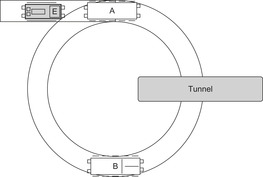 |
| Figure 1.3 |
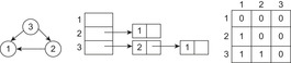
Looking at a state space problem in this way, it is immediately conducive to visualize it by drawing it. This leads to a graph-theoretical formalization, where we associate states with nodes and actions with edges between nodes. For the example problem, the state space is shown as a graph in Figure 1.4.
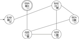 |
| Figure 1.4 |
Definition 1.1
(State Space Problem Graph) A problem graph  for the state space problem
  is defined by V = S as the set of nodes,
  as the initial node, T as the set of goal nodes, and
  as the set of edges that connect nodes to nodes with
  if and only if there exists an
  with
with  .
.
Note that each edge corresponds to a unique action, but often an action is specified in such a way that it can induce multiple edges. Each edge of the graph can be labeled by a respective action. In chess, for example, an action could be “move the king one square to the left,” and could be applied in many different positions with as many different outcomes. For the Railroad Switching problem, we could label the transitions by the sequence of executed actions of the engine; for example, (exit-right, couple-A, push-A, uncouple-A, cycle-left, couple-B, pull-B, exit-left, uncouple-B, exit-right, cycle-left) for the transition from state EAB to BAE. It is often possible to devise much smaller label sets.
Actions can be strung together into a sequence by applying an action to the result of another one. The objective of solving a state space problem is finding a solution.
Definition 1.2
(Solution) A solution  is an ordered sequence of actions
  ,
,  that transforms the initial state s into one of the goal states
  ; that is, there exists a sequence of states
  ,
,  , with
  ,
,  , and ui is the outcome of applying ai to ui−1,
  .
.
A solution for our example problem would be defined by the path (EAB, BAE, AEB, ABE, EBA). Note that several different solutions are possible, such as (EAB, BAE, BEA, ABE, EBA), but also as (EAB, BAE, BEA, ABE, AEB, BAE, AEB, ABE, EBA). Typically, we are not only interested in finding any solution path, but a shortest one—one with the minimum number of edges.
Frequently, we are not only interested in the solution length of a problem (i.e., the number of actions in the sequence), but more generally in its cost (again, depending on the application, authors use synonyms such as distance or weight). For the Railroad Switching example problem, costs could be given by travel time, distance, number of couplings/uncouplings, or power consumption. Each edge is assigned a weight. Unless stated otherwise, a key assumption we will make is that weights are additive; that is, the cost of a path is the sum of the weights of its constituting edges. This is a natural concept when counting steps or computing overall costs on paths from the initial state to the goal. Generalizations to this concept are possible and discussed later. The setting motivates the following definition.
Definition 1.3
(Weighted State Space Problem) A weighted state space problem is a tuple  , where w is a cost function
  . The cost of a path consisting of actions
  is defined as
  . In a weighted search space, we call a solution optimal if it has minimum cost among all feasible solutions.
For a weighted state space problem, there is a corresponding weighted problem graph  , where w is extended to
  in the straightforward way. The graph is uniform(ly weighted), if
  is constant for all
  . The weight or cost of a path
  is defined as
  .
.
Unweighted (or unit cost) problem graphs, such as the Railroad Switching problem, arise as a special case with  for all edges
  .
.
Definition 1.4
(Solution Path) Let  be a path in G. If
  and
and  for the designated start state s and the set of goal nodes T, then π is called a solution path. In addition, it is optimal if its weight is minimal among all paths between s and vk; in this case, its cost is denoted as
  . The optimal solution cost can be abbreviated as
  .
.
For example, the Railroad Switching problem has  . Solution paths to uniformly weighted problem graphs with
  for all edges
  are solved by considering the unit cost problem and multiplying the optimal solution cost with k.
1.5. Problem Graph Representations
Graph search is a fundamental problem in computer science. Most algorithmic formulations refer to explicit graphs, where a complete description of the graph is specified.
A graph  is usually represented in two possible ways (see Fig. 1.5). An adjacency matrix refers to a two-dimensional Boolean array M. The entry Mi,j,
  , is true (or 1) if and only if an edge contains a node with index i as a source and a node with index j as the target; otherwise, it is false (or 0). The required size of this graph representation is
  . For sparse graphs (graphs with relatively few edges) an adjacency list is more appropriate. It is implemented as an array L of pointers to node lists. For each node u in V, entry Lu will contain a pointer to a list of all nodes v with
  . The space requirement of this representation is
  , which is optimal.
 |
| Figure 1.5 |
Adding weight information to these explicit graph data structures is simple. In case of the adjacency matrix, the distance values are substituting the Boolean values so that entries Mi,j denote corresponding edge weights; the entries for nonexisting edges are set to ∞. In the adjacency list representation, with each node list element v in list Lu we associate the weight  .
.
Solving state space problems, however, is sometimes better characterized as a search in an implicit graph. The difference is that not all edges have to be explicitly stored, but are generated by a set of rules (e.g., in games). This setting of an implicit generation of the search space is also called on-the-fly, incremental, or lazy state space generation in some domains.
Definition 1.5
(Implicit State Space Graph) In an implicit state space graph, we have an initial node  , a set of goal nodes determined by a predicate Goal:
  , and a node expansion procedure Expand:
  .
.
Most graph search algorithms work by iteratively lengthening candidate paths  by one edge at a time, until a solution path is found. The basic operation is called node expansion (a.k.a. node exploration), which means generation of all neighbors of a node u. The resulting nodes are called successors (a.k.a. children) of u, and u is called a parent or predecessor (if un−1 additionally is a neighbor it might not be generated if expand is clever, but it can still be a successor). All nodes
  are called ancestors of u; conversely, u is a descendant of each node
  . In other words, the terms ancestor and descendant refer to paths of possibly more than one edge. These terms relate to the exploration order in a given search, whereas the neighbors of a node are all nodes adjacent in the search graph. To abbreviate notation and to distinguish the node expansion procedure from the successor set itself, we will write Succ for the latter.
An important aspect to characterize state space problems is the branching factor.
Definition 1.6
(Branching Factor) The branching factor of a state is the number of successors it has. If Succ(u) abbreviates the successor set of a state  then the branching factor is |Succ(u)|; that is, the cardinality of Succ(u).
In a problem graph, the branching factor corresponds to the out-degree of a node; that is, its number of neighbors reachable by some edge. For the initial state EAB in the Railroad Switching example, we have only one successor, whereas for state BAE we have a branching factor of 3.
For a problem graph, we can define an average, minimum, and maximum branching factor. The average branching factor b largely determines the search effort, since the number of possible paths of length l grows roughly as bl.
1.6. Heuristics
Heuristics are meant to be estimates of the remaining distance from a node to the goal. This information can be exploited by search algorithms to assess whether one state is more promising than the rest. We will illustrate that the computational search effort can be considerably reduced if between two candidate paths, the algorithm prefers to expand the one with the lower estimate. A detailed introduction to search algorithms is deferred to the next section.
A search heuristic provides information to orient the search into the direction of the search goal. We refer to the graph  of a weighted state space problem.
Definition 1.7
(Heuristic) A heuristic h is a node evaluation function, mapping V to  .
.
If  for all t in T and if for all other nodes
  we have
  , the goal check for u simplifies to the comparison of h(u) with 0.
Before plunging into the discussion of concrete examples of heuristics in different domains, let us briefly give an intuitive description of how heuristic knowledge can help to guide algorithms; the notions will be made precise in Chapter 2.
Let g(u) be the path cost to a node u and h(u) be its estimate. The value g(u) varies with the path on which u is encountered. The equation is very important in understanding the behavior of heuristic search algorithms. In words, the f-value is the estimate of the total path cost from the start node to the target destination, which reaches u on the same path.
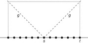
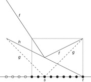
As general state spaces are difficult to visualize, we restrict ourselves to an extremely simplified model: the states are linearly connected along the horizontal axis, like pearls on a string (see Fig. 1.6). In each step, we can look at one state connected to a previously explored state.
 |
| Figure 1.6 |
If we have no heuristic information at all, we have to conduct a blind (uninformed) search. Since we do not know if the target lies on the left or the right side, a good strategy is to expand nodes alternatively on the left and on the right, until the target is encountered. Thus, in each step we expand a node of which the distance g from s is minimal.
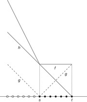
When a heuristic h is given, an extension of this strategy always prefers to expand the most promising node, the one of which the estimated total distance to the target,  , is minimal. Then, at least all nodes with f-value less than the optimal solution cost f* will be expanded; however, since h increases the estimate, some nodes can be pruned from consideration. This is illustrated in Figure 1.7, where h amounts to half the true goal distance. In a perfect heuristic, the two are identical. In our example (see Fig. 1.8), this reduces the number of expanded nodes to one-half, which is optimal.
 |
| Figure 1.7 |
 |
| Figure 1.8 |
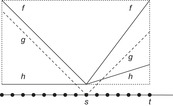
Finally, Figure 1.9 depicts the case of a heuristic that is misleading. The path going away from the goal looks better than the path to the goal. In this case, the heuristic search traversal will expand more nodes than blind exploration.
 |
| Figure 1.9 |
Heuristics are particularly useful if we can make sure that they sometimes may underestimate, but never overestimate, the true goal distance.
Definition 1.8
(Admissible Heuristic) An estimate h is an admissible heuristic if it is a lower bound for the optimal solution costs; that is,  for all
  .
.
Other useful properties of heuristics are consistency and monotonicity.
Definition 1.9
(Consistent, Monotonic Heuristic) Let  be a weighted state space problem graph.
• A goal estimate h is a consistent heuristic if  for all edges
  .
.
• Let  be any path, g(ui) be the path cost of
  , and define
  . A goal estimate h is a monotone heuristic if
  for all
  ,
,  ; that is, the estimate of the total path cost is nondecreasing from a node to its successors.
The next theorem shows that these properties are actually equivalent.
Theorem 1.1
(Equivalence of Consistent and Monotone Heuristics) A heuristic is consistent if and only if it is monotone.
Proof
For two subsequent states ui−1 and ui on a path  we have
| (by the definition of f) | |
| (by the definition of path cost) | |
| (by the definition of consistency) | |
| (by the definition of f) |
Moreover, we obtain the following implication.
Theorem 1.2
(Consistency and Admissibility) Consistent estimates are admissible.
Proof
If h is consistent we have  for all
  . Let
. Let  be any path from
  to
to  . Then we have
 This is also true in the important case of p being an optimal path from u to
  . Therefore,
  .
.
1.7. Examples of Search Problems
In this section, we introduce some standard search problems we will refer to throughout the book. Some of them are puzzles that have been used extensively in the literature for benchmarking algorithms; some are real-world applications.
1.7.1. Sliding-Tile Puzzles
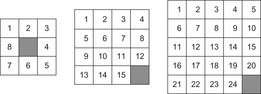
Our first example, illustrated in Figure 1.10, is a class of single-player sliding-tile toy games called the Eight-Puzzle, the Fifteen-Puzzle, the Twenty-Four-Puzzle, and, generally, the (n2 − 1)-Puzzle. It consists of  numbered tiles, squarely arranged, that can be slid into a single empty position, called the blank. The task is to rearrange the tiles such that a certain goal state is reached. The state space for these problems grows exponentially in n. The total number of reachable states1 is
  .
.
1The original version of this puzzle was invented by Sam Lloyd in the 1870s, and was made with 15 wooden blocks in a tray. He offered a reward of $1,000 to anyone who could prove they'd solved it from the state where the 14 and 15 were switched. All sorts of people claimed they had solved the puzzle, but when they were asked to demonstrate how they'd done it (without actually picking the blocks off the tray and replacing them), none of them could do it. Apparently, one clergyman spent a whole freezing winter night standing under a lamp post trying to remember what he'd done to get it right.Actually, there exists no solution for this; the concept that made Sam Lloyd rich is called parity. Assume writing the tile numbers of a state in a linear order, by concatenating, consecutively, all the rows. An inversion is defined as a pair of tiles x and y in that order such that x occurs before y in that order, but  . Note that a horizontal move does not affect the order of the tiles. In a vertical move, the current tile always skips over the three intermediate tiles following in the order, and these are the only inversions affected by that move. If one of these intermediate tiles contributes an inversion with the moved tile, it no longer does so after the move, and vice versa. Hence, depending on the magnitudes of the intermediate tiles, in any case the number of inversions changes by either one or three. Now, for a given puzzle configuration, let N denote the sum of the total number of inversions, plus the row number of the blank. Then
  is invariant under any legal move. In other words, after a legal move an odd N remains odd, whereas an even N remains even. Consequently, from a given configuration, only half of all possible states are reachable.
 |
| Figure 1.10 |
For modeling the puzzle as a state space problem, each state can be represented as a permutation vector, each of the components of which corresponds to one location, indicated by which of the tiles (including the blank) it occupies. For the Eight-Puzzle instance of Figure 1.10 the vector representation is  . Alternatively, we can devise a vector of the locations of each tile
  in the example. The last location in the vector representation can be omitted.
The first vector representation naturally corresponds to a physical  board layout. The initial state is provided by the user; for the goal state we assume a vector representation with value i at index
  ,
,  . The tile movement actions modify the vector as follows. If the blank is at index j,
  , it is swapped with the tile either in direction up (index
  ), down (index
  ), left (index
  ), or right (index
  ) unless the blank is already at the top-most (or, respectively, bottom-most, left-most, or right-most) fringe of the board. Here we see an instance where a labeled action representation comes in handy: We let Σ be
  with U, D, L, and R denoting a respective up, down, left, or right movement (of the blank). Although strictly speaking, up movements from a different blank position are different actions, in each state at most one action with a given label is applicable.
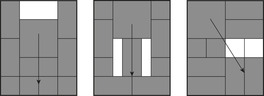
The General Sliding-Tile Puzzle (a.k.a. Klotzki) is an extension of the (n2 − 1)-Puzzle where the pieces can have different shapes. It consists of a collection of possibly labeled pieces to be slid on adjacent positions on a given board in either of the four directions up, down, left, and right. Each piece is composed of a set of tiles. Pieces of the same shape and labeling are indistinguishable. Figure 1.11 visualizes typical General Sliding-Tile Puzzle instances. The goal is to move the 2 × 2 block toward the arrow head. A compact representation is the list of tiles according to fixed reference coordinates and some traversal of the board. For the Donkey Puzzle example, and a natural reference spot and traversal of the board, we obtain the list 2x1, blank, blank, 2x1, 2x2, 2x1, 2x1, 1x2, 1x1, 1x1, 1x1, and 1x1. Let s, the total number of pieces, be partitioned into sets of fi pieces of the same type for  ; then the number of configurations is bounded by
  . The exact number can be determined utilizing a turn out of which the next piece to be placed is drawn. If a piece fits into the current configuration the next one is drawn, otherwise an alternative piece is chosen. With this approach we can compute the total state count for the puzzles: Dad's Puzzle, 18, 504; Donkey Puzzle, 65, 880; and Century Puzzle, 109, 260. A successor can be generated in time linear to the number of tiles (see Exercises).
 |
| Figure 1.11 |
One of the simplest heuristics for sliding-tile puzzles is to count the number of tiles that are not at their respective goal location. This misplaced-tile heuristic is consistent, since it changes by at most one between neighboring states.
The (n2 − 1)-Puzzle has another lower bound estimate, called the Manhattan distance heuristic. For each two states  and
and 
 , with coordinates
  it is defined as
  ; in words, it is the sum of moves required to bring each tile to its target position independently. This yields the heuristic estimate
  .
.
The Manhattan distance and the misplaced-tile heuristic for the (n2 − 1)-Puzzle are both consistent, since the difference in heuristic values is at most 1; that is,  , for all
  . This means
  and
and  . Together with
  , the latter inequality implies
  .
.
An example is given in Figure 1.12. Tiles 5, 6, 7, and 8 are not in final position. The number of misplaced tiles is 4, and the Manhattan distance is 7.
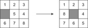
An improvement for the Manhattan distance is the linear conflict heuristic. It concerns pairs of tiles that both are in the correct row (column), but in the wrong order in column (row) direction. In this case, two extra moves not accommodated in the Manhattan distance will be needed to get one tile out of the way of the other one. In the example, tiles 6 and 7 are in a linear conflict and call for an offset 2 to the Manhattan distance. Implementing the full linear conflict heuristic requires checking the permutation orders for all pairs of tiles in the same row/column.
1.7.2. Rubik's Cube
Rubik's Cube (see Fig. 1.13), invented in the late 1970s by Erno Rubik, is another known challenge for a single-agent search. Each face can be rotated by 90, 180, or 270 degrees and the goal is to rearrange the subcubes, called cubies, of a scrambled cube such that all faces are uniformly colored. The 26 visible cubies can be classified into 8 corner cubies (three colors), 12 edge cubies (two colors), and 6 middle cubies (one color). There are  possible cube configurations. Since there are six faces—left (L), right (R), up (U), down (D), front (F), and back (B)—this gives an initial branching factor of
  . The move actions are abbreviated as L, L2, L−, R, R2, R−, U, U2, U−, D, D2, D−, F, F2, F−, B, B2, and B−. (Other notations consist of using ′ or −1 for denoting inverted operators, instead of −.)

We never rotate the same face twice in a row, however, since the same result can be obtained with a single twist of that face. This reduces the branching factor to  after the first move. Twists of opposite faces are independent of each other and hence commute. For example, twisting the left face followed by the right face gives the same result as twisting the right face followed by the left face. Thus, if two opposite faces are rotated consecutively, we assume them to be ordered without loss of generality. For each pair of opposite faces, we arbitrarily label one a first face and the other a second face. After a first face is twisted, there are three possible twists of each of the remaining five faces, resulting in a branching factor of 15. After a second face is twisted, however, we can only twist four remaining faces, excluding the face just twisted and its corresponding first face, for a branching factor of 12.
Humans solve the problem by a general strategy that generally consists of macro actions, fixed move sequences that correctly position individual or groups of cubes without violating previously positioned ones. Typically, these strategies require 50 to 100 moves, which is far from optimal.
We generalize the Manhattan distance to Rubik's Cube as follows. For all cubies, we cumulate the minimum number of moves to a correct position and orientation. However, since each move involves eight cubies, the result has to be divided by 8. A better heuristic computes the Manhattan distance for the edge and corner cubies separately, takes the maximum of the two, and divides it by 4.
1.7.3. Sokoban
Sokoban was invented in the early 1980s by a computer games company in Japan. There exists a set of benchmark problems (see Fig. 1.14), ordered roughly easiest to hardest in difficulty for a human to solve. The start position consists of n balls (a.k.a. stones, boxes) scattered over a maze. A man, controlled by the puzzle solver, traverses the board and pushes balls onto an adjacent empty square. The aim is to move the balls onto n designated goal fields.
 |
| Figure 1.14 |
One important aspect of Sokoban is that it contains traps. Many state space problems like the Railroad Switching problem are reversible; that is, for each action  there exists an action
  , so that
  and
and  . Each state that is reachable from the start state can itself reach the start state. Hence, if the goal is reachable, then it is reachable from every state. Directed state space problems, however, can include dead-ends.
Definition 1.10
(Dead-End) A state space problem has a dead-end  if u is reachable and
  is unsolvable.
Examples for dead-ends in Sokoban are four balls placed next to each other in the form of a square, so that the man cannot move any of them; or balls that lie at the boundary of the maze (excluding goal squares). We see that many dead-ends can be identified in the form of local patterns. The instance in Figure 1.14, however, is solvable.
For a fixed number of balls, the problem's complexity is polynomial. In general, we distinguish three problems: Decide is just the task to solve the puzzle (if possible), Pushes additionally asks to minimize the number of ball pushes, whereas Moves request an optimal number of man movements. All these problems are provably hard (PSPACE complete).
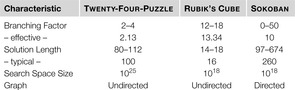
We see that complexity theory states results on a scaling set of problems, but does not give an intuitive understanding on the hardness for a single problem at hand. Hence, Figure 1.15 compares some search space properties of solitaire games. The effective branching factor is the average number of children of a state, after applying pruning methods. For Sokoban, the numbers are for typical puzzles from the humanmade test sets; common Sokoban board sizes are  .
.
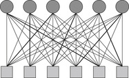
One good lower bound estimate for Sokoban (Pushes variant) is found using a minimal matching approach. We are interested in a matching of balls to goal fields, such that the sum of all ball paths is minimal. The one part of the bipartite graph (see Fig. 1.16) is composed of nodes for the balls, the other half consists of nodes for the goal fields, and the edge weight between every selected pair (ball, goal) of nodes is the shortest path cost for moving the ball to goal (assuming all other balls were removed from the problem). The standard algorithm to compute the best weighted matching runs in time cubic in the number of balls. More efficient algorithms reduce the problem to the maximum flow problem by inserting additional start and sink nodes connected to the ball nodes and to the goal fields, respectively.
 |
| Figure 1.16 |
In the case of a group of goal fields that is only reachable via a single door, the minimal matching heuristic can be simplified as shortest path calculations through this articulation (an articulation of a connected graph is a node that if removed will disconnect the graph). The heuristic is consistent, since moving one ball reduces the individual shortest path to each goal by at most one, and any matching will include only one of the updated shortest path distance values.
1.7.4. Route Planning
A practically important application domain for search algorithms is Route Planning. The (explicit) search graph consists of a road network, where intersections represent nodes and edges represent drivable connections. The graph is relatively sparse, since the degree of nodes is bounded (intersections with five or more participating roads are very rare). The task consists of finding a path between a start location s and a target location t that minimizes distance, expected travel time, or a related measure. A common approach to estimate travel time is to classify roads into a number of road classes (e.g., freeway, highway, arterial road, major road, local connecting road, residential street), and to associate an average speed with each one. The problem can become challenging in practice due to the large size of maps that have to be stored on external memory, and on tight time constraints (e.g., of navigation systems or online web search). In Route Planning, nodes have associated coordinates in some coordinate space (e.g., the Euclidean). We assume a layout function  . A lower bound for the road distance between two nodes u and v with locations
  and
and  can be obtained as
  , where
  denotes the Euclidean distance metric. It is admissible, since the shortest way to the goal is at least as long as the beeline. The heuristic
  is consistent, since
 by the triangle inequality of the Euclidean plane.
1.7.5. TSP
One other representative for a state space problem is the TSP (traveling salesman problem). Given a distance matrix between n cities, a tour with minimum length has to be found, such that each city is visited exactly once, and the tour returns to the first city. We may choose cities to be enumerated with  and distances
  and
and  for
for  . Feasible solutions are permutations τ of
  and the objective function is
  and an optimal solution is a solution τ with minimal
  . The state space has
  solutions, which is about
  for
for  . This problem has been shown to be NP complete in the general case; entire books have been dedicated to it. Figure 1.17 (left) shows an example of the TSP problem, and Figure 1.17 (right) a corresponding solution.
 |
| Figure 1.17 |
Various algorithms have been devised that quickly yield good solutions with high probability. Modern methods can find solutions for extremely large problems (millions of cities) within a reasonable time with a high probability just 2 to 3% away from the optimal solution.
In the special case of the Metric TSP problem, the additional requirement of the triangle inequality is imposed. This inequality states that for all vertices u, v, and w, the distance function d satisfies  . In other words, the cheapest or shortest way of going from one city to another is the direct route between two cities. In particular, if every city corresponds to a point in Euclidean space, and distance between cities corresponds to Euclidean distance, then the triangle inequality is satisfied. In contrast to the general TSP, Metric TSP can be 1.5-approximated, meaning that the approximate solution is at most 50% larger than the optimal one.
When formalizing TSP as a search problem, we can identify states with incomplete tours, starting with any arbitrary node. Each expansion adds one more city to the partial path. A state denoting a completed, closed tour is a goal state.
A spanning tree of a graph is a subgraph without cycles connecting all nodes of the graph. A Minimum Spanning Tree (MST) is a spanning tree such that the sum of all its edge weights is minimum among all spanning trees of the graph. For n nodes, it can be computed as follows. First, choose the edge with minimum weight and mark it. Then, repeatedly find the cheapest unmarked edge in the graph that does not close a cycle. Continue until all vertices are connected. The marked edges form the desired MST.
A heuristic that estimates the total length of a TSP cycle, given a partial path, exploits that the yet unexplored cities have to be at least connected to the ends of the existing part (to both the first and the last city). So if we compute a MST for these two plus all unexplored cities, we obtain a lower bound for a connecting tree. This must be an admissible heuristic, since a connecting tree that additionally fulfills the linearity condition cannot be shorter. A partial solution and the MST used for the heuristic are shown in Figure 1.18.

1.7.6. Multiple Sequence Alignment
The Multiple Sequence Alignment problem, in computational biology, consists of aligning several sequences (strings; e.g., related genes from different organisms) to reveal similarities and differences across the group. Either DNA can be directly compared, and the underlying alphabet Σ consists of the set {C,G,A,T} for the four standard nucleotide bases cytosine, guanine, adenine and thymine; or we can compare proteins, in which case Σ comprises the 20 amino acids.
Roughly speaking, we try to write the sequences one above the other such that the columns with matching letters are maximized; thereby, gaps (denoted here by an additional letter _) may be inserted into either of them to shift the remaining characters into better corresponding positions. Different letters in the same column can be interpreted as being caused by point mutations during the course of evolution that substituted one amino acid by another one; gaps can be seen as insertions or deletions (since the direction of change is often not known, they are also collectively referred to as indels). Presumably, the alignment with the fewest mismatches reflects the biologically most plausible explanation.
The state space consists of all possible alignments of prefixes of the input sequences  . If the prefix lengths serve as vector components we can encode the problem as a set of vertices
  ,
,  with associated cost vector vx. A state x′ is a (potential) successor of x if
  for all i. The underlying problem graph structure is directed and acyclic and follows a k-dimensional lattice or hypercube.
There is a host of applications of sequence alignment within computational biology; for example, for determining the evolutionary relationship between species, for detecting functionally active sites that tend to be preserved best across homologous sequences, and for predicting three-dimensional protein structures.
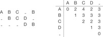
Formally, we associate a cost with an alignment and try to find the (mathematically) optimal alignment, the one with the minimum cost. When designing a cost function, computational efficiency and biological meaning have to be taken into account. The most widely used definition is the sum-of-pairs cost function. First, we are given a symmetric  matrix containing penalties (scores) for substituting a letter with another one (or a gap). In the simplest case, this could be one for a mismatch and zero for a match, but more biologically relevant scores have been developed. A substitution matrix corresponds to a model of molecular evolution and estimates the exchange probabilities of amino acids for different amounts of evolutionary divergence. Based on such a substitution matrix, the sum-of-pairs cost of an alignment is defined as the sum of penalties between all letter pairs in corresponding column positions. An example of the calculation of the sum-of-pairs cost is depicted in Figure 1.19. The value
  is based on entry (A/_) in the substitution matrix, and the second value 7 is based on entry (B,_) plus 1 for a still-opened gap.
 |
| Figure 1.19 |
A number of improvements can be integrated into the sum-of-pairs cost, like associating weights with sequences, and using different substitution matrices for sequences of varying evolutionary distance. A major issue in Multiple Sequence Alignment algorithms is their ability to handle gaps. Gap penalties can be made dependent on the neighbor letters. Moreover, it has been found that assigning a fixed score for each indel sometimes does not produce the biologically most plausible alignment. Since the insertion of a sequence of x letters is more likely than x separate insertions of a single letter, gap cost functions have been introduced that depend on the length of a gap. A useful approximation is affine gap costs, which distinguish between opening and extension of a gap and charge  for a gap of length x, for appropriate a and b. Another frequently used modification is to waive the penalties for gaps at the beginning or end of a sequence. A real alignment problem is shown in Figure 1.20.
 |
| Figure 1.20 |
The sequence alignment problem is a generalization of the problem of computing the edit distance, which aims at changing a string into another by using the three main edit operations of modifying, inserting, or deleting a letter. Each edit operation is charged, and the minimum-cost operations sequence is sought. For instance, a spell checker could determine the lexicon word of which the edit distance from a (possibly misspelled) word typed by the user is minimal. The same task arises in version control systems.
Lower bounds on the cost of aligning k sequences are often based on optimal alignments of subsets of  sequences. In general, for a vertex v in k-space, we are looking for a lower bound for a path from v to the target corner t. Consider first the case
  . The cost of such a path is, by definition, the sum of its edge costs, where each edge cost in turn is the sum of all pairwise (replacement or gap) penalties. Each Multiple Sequence Alignment induces a pairwise alignment for sequences i and j, by simply copying rows i and j and ignoring columns with a "_ ” in both rows.
By exchanging the summation order, the sum-of-pairs cost is the sum of all pairwise alignment costs of the respective paths projected on a face, each of which cannot be smaller than the optimal pairwise path cost. Thus, we can construct an admissible heuristic hpair by computing, for each pairwise alignment and for each cell in a pairwise problem, the cheapest path cost to the goal node.
The optimal solutions to all pairwise alignment problems needed for the lower-bound h values are usually computed prior to the main search in a preprocessing step. Since this time we are interested in the lowest cost of a path from v to t, it runs in a backward direction, proceeding from the bottom-right corner to the top-left corner in the alingment matrix, expanding all possible parents of a vertex in each step.
1.8. General State Space Descriptions
In this section, we introduce some general formalisms to describe state space problems: action planning, production systems, and generic search models including nondeterministic search and Markov decision processes.
1.8.1. Action Planning
Action planning refers to a world description in logic. A number of atomic propositions AP describe what can be true or false in each state of the world. By applying operations in a state, we arrive at another state where different propositions might be true or false. For example, in a Blocksworld a robot might try to reach a target state by actions that stack and unstack blocks, or put them on the table. Usually, only a few atoms are affected by an action, and most of them remain the same. Therefore, a concise representation is the following Strips formalism.
Definition 1.11
(Propositional Planning Problem) A propositional planning problem (in Strips notation) is a finite-state space problem  , where
  is the set of states,
  is the initial state,
  is the set of goal states, and A is the set of actions that transform states into states. We often have that T is described by a simple list of propositions
  . Actions
  have propositional preconditions pre(a), and propositional effects
  , where
  is the precondition list of a,
  is its add list, and
  is the delete list. Given a state u with
  , then its successor
  is defined as
  .
.
Effects are seen as updates to the current states. To avoid conflicts, delete effects are eliminated from the state before add effects are included.
Even though we have defined Strips on sets of propositions it is not difficult to transfer the description into logic. Boolean variables for propositions are called facts. The goal condition is shorthand for  and preconditions are interpreted as
  . The application of the add and delete lists are short for setting p to false for all
  followed by setting p to true for all
  . Strips planning assumes a closed world. Everything that is not stated true is assumed to be false. Therefore, the notation of the initial state s is shorthand for the assignment to true of the propositions included in s, and to false of the ones that are not.
It is often not difficult to encode a state space problem in Strips. For modeling the (n2 − 1)-Puzzle we introduce atomic propositions  , denoting the truth of the tile t to be located at position p, and
  , denoting that the blank is located at position p. An action would be
  , which has
  and
and  as preconditions,
  and
and  as add effects, as well as
  and
and  as delete effects.
To encode finite-domain state space problems with numbers, we observe that a variable with k possible value assignment can be encoded with O(lgk)(logarithmic encoding)—or O(k)(unary encoding)—atomic propositions. Of course, this is only feasible if k is small.
In Blocksworld (see Fig. 1.21) there are labeled blocks that can be moved using a robot arm that can grasp one block at a time. Additionally, there is a table large enough to hold all blocks. The four operations are stack (put block onto one tower), unstack (remove block from one tower), pickup (remove block from table), and putdown (put block onto table). Let us consider a Blocksworld problem with l blocks  placed on a table t as an example. State variables for each block are on that can take values from
  , a Boolean variable clear for each block, and an additional variable holding that can take values from
  . Actions are stack, unstack, putdown, pickup; for example, stack
  has preconditions
  and
and  and the four update operations
  ,
,  ,
,  , and
, and  . In a unary encoding, for each block a and b we devise the fluents
  ,
,  , and
, and  . The corresponding Strips action for
  has the two preconditions
  and
and  , the two add effects
  and
and  , as well as the two delete effects
  and
and  .
.
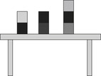
Planning domains can either beparametricor grounded (fully instantiated). Parametric descriptions feature predicates and actions based on a bounded number of domain objects. A (Lisp -like) formal representation for both parametric or grounded planning problems is referred to as the problem domain description language (PDDL). A PDDL example for a more complex Logistics domain illustrated in Figure 1.22 is provided in Figure 1.24. The task is to transport packages within cities using trucks, and between cities using airplanes. Locations within a city are connected and trucks can move between any two such locations. In each city there is exactly one truck, and each city has one airport. The airports are connected for airplanes to operate. One particular problem instance is shown in Figure 1.23.
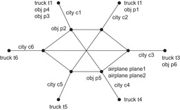
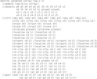
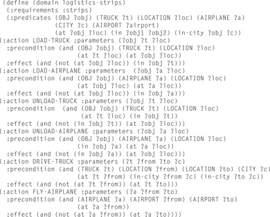
Strips-type planning is known to be PSPACE complete. Including types, numbers, and durations to the problem description in the developments of PDDL leads to specification formalisms that are undecidable. Nonetheless, there are enumeration algorithms and acceleration techniques that are practical for a large set of benchmarks. In recent years, the performance of state-of-the-art systems has improved drastically, and with that, more realistic examples came within reach. We have devoted an entire application chapter to address these developments (See Chapter 15, “Action Planning”).
Next, we present the relaxed planning heuristic h+ for planning in Strips notation with each action a, having precondition list  , add list
  , and delete list
  .
.
The relaxation a+ of an action a is a with the delete list omitted. The relaxation of a planning problem is the one in which all actions are substituted by their relaxed counterparts. Any solution that solves the original plan also solves the relaxed one. Value h+ is defined as the length of the shortest plan that solves the relaxed problem. This heuristic is consistent: The relaxed plan starting at v with cost  can be extended to a plan from u by adding the action that leads from u to v. Therefore, we have
  .
.
Solving relaxed plans is still computationally hard. It can, however, efficiently be approximated by the number of actions in a parallel plan that solves the relaxed problem. The polynomial time algorithm builds a relaxed problem graph followed by a greedy plan generation process. A pseudo-code implementation is provided in Algorithm 1.1. The variables l and i denote the layer for the forward and the backward phases, respectively.
An illustration for its work is given in Figure 1.25. The graph consists of five (encircled) layers for propositions, the last one containing the only goal. Layers are connected by actions. Propositions are identified with nodes and actions are identified with rectangles. Dotted lines denote the application of noop, an additional action that incurs no change. Propositions and actions in the relaxed plan are shaded.
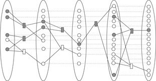
The first phase constructs the layered graph of propositional facts, performing a fixpoint computation on  starting with the initial state. In layer i all facts are considered that are reachable by applying an action with satisfied precondition facts in any layer j with
  . In layer 0 we have all facts present in the initial state. Since we have a finite number of grounded propositions the process eventually reaches a fixpoint. The next loop marks the goal facts.
The second phase is the greedy plan extraction phase. It performs a backward search to match facts to enabling actions. The goal facts build the first unmarked facts. As long as there are unmarked facts in layer i, select an action that makes this fact true and mark all add effects, and queue all preconditions as unmarked new goals. If there is no unmarked fact left in layer i, continue with layer i−1 until the only unmarked facts are the initial ones in layer 0. The heuristic is constructive; that is, it not only returns the estimated distance but also a corresponding sequence of actions.
The heuristic is neither admissible nor consistent, but it is effective in practice, especially for structurally simpler benchmark problems (problem graphs with no or recognized dead-end and small plateaus).
1.8.2. *Production Systems
Definition 1.12
(Production System) A production system is a state space problem  , of which the states are strings over the alphabet Σ, and the actions are given in form of grammar inference rules
  , with
  being strings over Σ.
The following theorem shows that any Turing machine computation can be casted as a special kind of a production system.
Theorem 1.3
(Undecidability for Production Systems) The problem to solve a general production system for arbitrary start and goal state is undecidable.
Proof
The proof is done via reduction to the halting problem for Turing machines. Given a Turing machine  with input alphabet
  , tape alphabet
  ,
,  , initial state q0, transition function
  , and goal state set
  , we construct a state space problem as follows.
States are configurations of the Turing machine M; that is, words of  . (With “*” we denote Kleene's hull: For a single letter σ, the term σ* refers to the set
  , where
  is the empty word. For all
  we have
  .)
.)
The initial state is state  and the goal state is
  . Depending on the value of d we assign each
  to words
  ,
,  ,
,  ,
,  with
with  and
and  . For
. For  we have
  ; for
; for  we have
  ; and for
  we have
  . Last, but not least, the rules
  and
and  shorten the empty tape. Hence, we have deduced that M halts on an empty input tape starting from q0 in finitely many steps in terminal state qe if and only if the initial state
  can be transformed into goal state
  in finitely many steps.
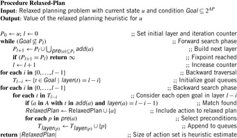
However, individual state space problems, including the ones with finite-state spaces, are decidable, so that most combinatorial problems like instances to the (n2 − 1)-Puzzle are solvable by general node expanding algorithms.
A convenient though less expressive formalism than general production systems is PSVN, or vector notation for productions systems. It is defined by a triple  , where s is a seed state, A is the set of actions, and L is the finite set of labels. States are represented by fixed-length vectors of labels from L. For example, the states of the Three-Puzzle (the (n2 − 1)-Puzzle for
  ) can be described as a 4-tuple, of which the components are chosen out of
  to indicate which tile is located at the top-left, top-right, bottom-left, and bottom-right squares, respectively. Actions are defined by a left-hand side (LHS), representing the precondition, and a right-hand side (RHS), defining the resulting state. Each side has the same length as the state vector. The semantics are defined in a way resembling Prolog unification rules; each position can hold a constant, a named variable, or an unnamed variable, denoted "_”. A constant in LHS represents an exact match for a state at that position. A named variable in LHS represents a binding of the label in the state to which LHS is being applied, and basically leaves a label unchanged. Every variable of RHS must be bound in LHS and every constant label must belong to the set of declared labels. The state space is the transitive closure of applying any sequence of actions to s.
For example, consider the following action definition  . The action applies to states of which the first two labels are identical and the third label is 1. The fifth and sixth labels are bound to B and C, respectively. Applying a to state
  results in
  . In the Three-Puzzle, the action
  moves the blank from the top-left to the top-right square.
1.8.3. Markov Decision Processes
Markov decision process problems (MDPs) assume a finite number of states and actions. At each time the agent observes a state and executes an action, which incurs intermediate costs to be minimized (or, in the inverse scenario, rewards to be maximized). The cost and the successor state depend only on the current state and the chosen action. Successor generation may be probabilistic, based on the uncertainty we have on the environment in which the search takes place. For example, an action might sometimes fail to result in the desired target state, instead staying in the current state with a small probability.
We should point out that in this book we assume that we always have perfect knowledge of what state we are in. This assumption is dropped in the concept of a partially observable Markov decision process problem (POMDP). Here, instead, we are given some observations based on which we can estimate the probability of being in a certain state.
Definition 1.13
(MDP) A Markov decision process problem is a tuple  , where S is the underlying state space, A is the set of actions,
  is the cost or immediate reward function, and
  is the probability that action a in state u will lead to state v. In some MDPs, additional costs c incur when arriving at a goal state. The goal is to minimize the (expected) accumulated costs or, equivalently, to maximize the (expected) accumulated rewards.
As Markov decision processes are defined on sequences of actions they are an extension of Markov chains.
Definition 1.14
(Policy) A solution to an MDP is provided in terms of a policy π, which maps each state to an action to take in this state.
In some cases the policy may be realized by means of a lookup table, whereas in others it may involve extensive computation. Applying action a in u incurs costs  . The goal is to minimize the expected costs
  for a state u over the set of all possible policies π, where the value function
  at u is often called expected return, starting from u. The optimal value function is denoted by f*.
1.8.4. Generic Search Model
A generalized model of a state space search problem consists of a discrete and finite-state space S, an initial state s, and a nonempty set of terminal states T. Furthermore, a set of actions  applicable in each nonterminal state u, an action cost function
  for nonterminal states, and a terminal cost function
  are assumed. In the general case, X is a real-valued cost function, but in many practical cases X is a small set of integers.
In deterministic models, the successors of a node u are  . For the nondeterministic search model, we have
  . Successor outcomes are either added or maximized. For MDPs with probabilities
  we have that
  .
.
A simple example of an MDP is a probabilistic version of the (n2 − 1)-Puzzle with noisy actions that achieve their intended effects with probability  and have no effect with probability
  .
.
The solutions to the models can be expressed in terms of Bellman equations, which induce options to compute optimal policies. For the deterministic case we have For the nondeterministic case we have either (additive model)
 or (max model)
 For the MDP case we have
In a unified perspective, the functions f* are solutions to the set of Bellman equations, and, hence, optimal value functions. Policies  for the nondeterministic and probabilistic cases are extensions of plans that map states to actions. In practice, they are used in the form of controllers to simulate the solution process. Policies are greedy if they match any given value function, and policies π* that are greedy with respect to the optimal value function are called optimal.
For the deterministic setting, the outcome of applying an action is unique, such that π can be reduced to a sequence of states. In this case the optimal value function f* exactly estimates the total distance from each state to a goal state; that is, and the optimal plan π* is the one that minimizes its total cost; that is,
In some implementations, the update is performed on the Q-value  , an intermediate term in the preceding equations, which also depends on the model. It is defined for deterministic models as
 for nondeterministic (additive and max) models as
 and for MDPs as
1.9. Summary
In this chapter, we introduced the kinds of problems that we study in most chapters of this book, namely graph search problems where we are given a weighted directed graph (where edges are directed and have a cost), a start node, and a set of goal nodes, and the objective is to find a shortest path in the graph from the start node to any goal node. We introduced the terminology used in artificial intelligence for such graph search problems. The nodes, for example, are called states and the edges are called actions. We then discussed ways of categorizing graphs, for example, their branching factor (the number of outgoing edges averaged over all nodes). We also discussed two ways of representing graphs, namely explicitly (by enumerating all nodes and edges) and implicitly (by giving a procedure of which the input is a node and the output is a list of outgoing edges together with the nodes that they point to). Implicit graph representations can be problem-specific or general, for example, using Strips or production systems. Implicit representations can be much more compact than explicit representations, which allow implicit representations to represent large graph search problems by exploiting their structure. However, a shortest path can be found in time polynomial in the size of an explicit representation, but often not in time polynomial in the size of an implicit representation.
We then discussed several problems that can be formulated as graph search problems, some of which are used as typical test domains for graph search algorithms and some of which are important in practice, including for transportation systems and biology. In many of these domains, the shortest path is important since it allows one to move from the start node to a goal node. In some domains (e.g., in the TSP), however, only the goal node reached by the shortest path is important since it encodes how to move. To be efficient, graph search algorithms need to exploit some knowledge of the graphs they search. This knowledge can be provided by the domain expert in the form of encoding the heuristic function manually, or, as illustrated later in this book, obtained automatically from the problem structure.
Table 1.1 gives an overview on the state space problems in this chapter and their characteristics (implicit/explicit graph, reversible/irreversible actions, range of weight function, complexity). These search problems dominate the content of the book but are not the only ones that we discuss; we also discuss different two-player games.
One powerful piece of knowledge for solving state space problems is a heuristic. A heuristic assigns a heuristic value to every node, where a heuristic value is an estimate of the goal distance of the node (the length of a shortest path from the node to any goal node). Good heuristics are close to the goal distances and fast to calculate. They can be found easily for most graph search problems. Two important properties are their admissibility (does not overestimate the goal distances) and consistency (satisfies the triangle inequality), where consistency implies admissibility. In Chapter 2, we introduce a graph search algorithm that is able to exploit a given heuristic.
Table 1.2 depicts the properties of the heuristics that have been introduced. Additionally, we show the order of runtime for computing the heuristic estimate for a state (measured in the size of the state vector).
Some heuristics (e.g., the relaxed planning or the Euclidean distance) do not shrink the problem graph but introduce new edges. In other heuristics (e.g., the Manhattan distance or minimal matching), sets of nodes are contracted to super-nodes, and adjacent edges are merged (the principle will be reconsidered in Chapter 4). One problem in deriving well-informed heuristics based on problem projections is to devise problem simplifications, so that the individual estimates based on solving the subproblems can be added admissibly.
1.10. Exercises
1.1 Write a Turing machine program in pseudo code for the following problems:
1. Addition of two numbers in unary representation.
2. Increment of a number in binary representation.
3. Decrement of a number in binary representation.
4. Addition of two numbers in binary representation (use parts (b) and (c)).
1.2
1. Determine constants c and n0, to show  .
.
2. If the limit of  for large n is bounded by a constant c we have that
  . Use this result to show
  .
.
3. The Rule of L'Hˆopital states that if the limit of  for large n is bounded then it is equal to the limit of
  for large n. Use this rule to prove
  .
.
1.3 Prove thebig-oh
1. addition rule: 
2. multiplication rule:  , for given functions f and g.
Explain the practical use of the rules.
1.4
1. Let a, b, c be real values with  . Show
  .
.
2. Let p(n) be a polynomial of constant degree k. Show  .
.
3. Show  and, more generally,
  for all
  .
.
1.5 Show that according to the definition of ≐
1. 
2. 
1.7 Show that the bit-flipping efforts for a binary counter according to the following table are amortized constant.
| Step | Operation | Φi | ti | |
| 0 | 0 | |||
| 0 | ↓ | 1 | 2 | |
| 1 | 1 | |||
| 1 | ↓ | 2 | 2 | |
| 10 | 1 | |||
| 2 | ↓ | 1 | 2 | |
| 11 | 2 | |||
| 3 | ↓ | 3 | ||
| 100 | 1 | |||
| 4 | ↓ | 1 | 2 | |
| 101 | 2 | |||
| 5 | ↓ | 2 | 2 | |
| 110 | 2 | |||
| 6 | ↓ | 1 | 2 | |
| 111 | 3 | |||
| 7 | ↓ | 4 | ||
| 1000 | 1 | |||
| 8 | ↓ | 1 | 2 | |
| 1001 | 2 |
1.8 The pseudo code we consider uses different loop and case statements. Show that
1. for  〈B〉
〈B〉
2. do 〈B〉while (〈A〉)
3. if (〈A〉)〈B〉else 〈C〉
are all syntactic sugar and can be expressed with a classic while loop.
1.9 The Fibonacci numbers are recursively defined as follows:
Show by induction that
1. for  we have
2. for  we have
3. for  we have

1.11 Use a truth table to show
1. 
2. 
1.12 Given four pieces of chain (initial state shown in Fig. 1.26, left), the Cheap Necklace problem is characterized as follows. It costs 20 cents to open and 30 cents to close a link. Join all links into a single necklace (goal state in Figure 1.26, right) at the lowest cost.
1. What are the states? What are the actions? What is the start state? What are the goal states? What are the weights? What are the costs for an optimal solution?
2. How many states are there? What is the average branching factor?
3. Is the graph directed or undirected? Does the graph contain dead-ends?
1.13 For the General Sliding-Tile Puzzle:
1. Compute the number of reachable system states for the instances of Figure 1.27. In the Harlequin Puzzle (left) the two corner pieces have to be assembled to a  block. In the Man and Bottle Puzzle (right), the man at the left side has to move to the right next to the bottle.
2. Give a suitable generalization of the Manhattan distance heuristic.
3. Show that the test for successor generation can be performed in total time linear to the number of tiles (counting blanks as empty tiles).
1.14 Consider the example level in Sokoban shown in Figure 1.14.
1. Determine an optimal solution for Pushes and for Moves.
2. Show that, in general, optimal solutions for both problems differ.
1.16 For Blocksworld:
1. Model the problem of Figure 1.21 in Strips using the predicates on, clear, and holding.
2. Show that finding a solution that is at most twice as long as the optimal one can be computed in polynomial time.
1.17 Another scalable sliding-tile puzzle Frogs and Toads invented by Gardner additionally allows tile jumps (see Fig. 1.28). The goal is to exchange the sets of black and white tiles in the minimum number of moves.
1. Give a state space characterization of the puzzle.
2. Determine the number of reachable configurations in a formula depending on n.
3. Devise a heuristic for the puzzle.
1.18 The goal of Atomix (see Fig. 1.29) is to assemble a given molecule from atoms. The player can select an atom at a time and push it toward one of the four directions left, right, up, and down; it will keep moving until it hits an obstacle or another atom. The game is won when the atoms form the same constellation (the molecule) as depicted beside the board. Note that the interconnection of the atoms matters.
1. Formalize Atomix as a state space problem.
2. Extend Figure 1.15 with the characteristics of Atomix.
3. Obtain an easily computable heuristic that allows an atom to slide through other atoms or share a place with another atom.
4. Find a solution for Figure 1.29.
1.19 An n-Wusel (see Fig. 1.30) consists of n connected blocks. In motion, a group of blocks is simultaneously moved. The possible directions are left, right, up, down, forward, and backward. A move group is connected. An example for a sequence of moves is given in Figure 1.31.
Cubes connected to the ground can only be moved upward. At least one block has to stay on the ground. All other blocks have to be arranged such that the Wusel is in balance. The Wusel tumbles if the projection of the center of mass is outside the convex hull of the blocks on the floor (the convex hull includes all points on lines between any two points).
1. Give a (coarse) estimate for the number of n-Wusels.
2. Choose an appropriate representation that allows fast connectivity checks.
3. Find out how to efficiently perform stability checks for the Wusel.
4. Devise an efficient function for a successor generation.
5. Devise a heuristic estimate for the Wusel wrt. a target location for the center of mass.
1.21 Test your structural knowledge on heuristics.
1. Prove that the maximum of several consistent heuristics is a consistent heuristic.
2. Show that the sum of two consistent estimates is not necessarily admissible.
3. Give an example of an admissible heuristic that is not consistent.
1.22 Devise a PSVN characterization of the state and state change for the Rubik's Cube.
1.23 Prove that a PSVN action is reversible, if and only if there is no i such that the label at i of the left side is _, the label at i of the right side is different to _, and every variable bound on the left side is present on the right side; that is, if it is used to assign a label on the right side, or if there is a j so that the label at j on the left side is some variable A, and on the right side, it is either _ or A.
1.24 The cross-product state space  of the state space problems
  is defined as
  ,
,  ,
,  , and
, and  . Let heuristic hi be the minimal solution length from the current local state Si to reach a goal in Ti for problem Pi. Show that hi is consistent.
1.25 Devise an MDP model for a variant of the the (n2 − 1)-Puzzle domain, where each intended move fails with a probability of 10%.
1.26 An instance of the pen-and-paper game Racetrack is defined by a racetrack divided into grid cells together with cars initially standing behind a starting line. The goal is to cross an additional finish line. The task is to find the control for driving a car from an initial state into a set of goal states, minimizing the number of time steps and without hitting the racetrack's boarder. Each applied action achieves its intended effect with probability 0.7. Provide an MDP model for Racetrack with states consisting of coordinates  and velocity vectors
  .
.

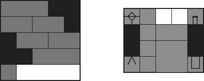
 |
| Figure 1.28 |


1.11. Bibliographic Notes
Milestones in single-agent games refer to publications of Korf (1985a), Korf and Schultze (2005) (Fifteen-Puzzle), Korf and Felner (2002), Korf and Taylor (1996) (Twenty-Four-Puzzle), Edelkamp et al. (2008b) (Thirty-Five-Puzzle), Korf and Felner (2007) (Towers-of-Hanoi), Junghanns (1999) (Sokoban) and Korf (1997), Kunkle and Cooperman (2008) (Rubik's Cube). Reid has shown in 1995 that the one position (corners correct, edges placed but flipped) requires at least 20 moves; the according lower bound has been proven in 2010 by Rokicki, Kociemba, Davidson, and Dethridge. 2 The presentation of multiplayer game efficiencies refers to the work of Campbell et al. (2002) (Chess), Schaeffer et al. (2005) and Schaeffer et al. (2007) (Checkers), Tesauro (1995) (Backgammon), Allis (1998), Allen (2010), Tromp (2008) (Connect 4), and Ginsberg (1999) and Smith et al. (1998) (Bridge). The number 4,531,985,219,092 computed by Edelkamp and Kissmann (2008b) for Connect 4 has been validated by John Tromp in 2010. Large-scale search in probabilistic environments has been studied by Edelkamp et al. (2007).
The set of remarkable results in planning have been published in the context of the international planning competitions. Parallel optimal planning has been addressed by Blum and Furst (1995) and Kautz and Selman (1996), while sequential optimal planning has been considered by Helmert et al. (2007), among others. UCT for general game playing goes back to Kocsis and Szepesvári (2006).
Multiple sequence alignment problems have been solved with AI search methods by Edelkamp and Kissmann (2007) and Korf and Zhang (2000), Schrödl (2005) and Zhou and Hansen (2002b). Recent entries to verification via AI search are given by Edelkamp et al. (2004b) (explicit-state model checking), Bloem et al. (2000) (hardware verification), Groce and Visser (2002) (program model checking), Jabbar (2008) (external model checking), Wijs (1999) (quantitative model checking), and Kupferschmid et al. (2007) (real-time model checking). Vehicle navigation results refer to work by Wagner and Willhalm (2003), Bast et al. (2007) (maps), Edelkamp et al. (2003) and Schrödl et al. (2004) (GPS). From the broad range of applying search in robotics we highlighted results of Gutmann et al. (2005) and Henrich et al. (1998).
The motivating example is taken from Wickelgren (1995). Ratner and Warmuth (1990) have shown that optimally solving the (n2 − 1)-Puzzle is NP-hard. First optimal solutions to the Eight-Puzzle have been provided by Schofield (1967), for the Fifteen-Puzzle by Korf (1985a) and for the Twenty-Four-Puzzle by Korf and Taylor (1996), with an improvement by Korf and Felner (2002). The General Sliding-Tile Puzzle problems are either commercially available or taken from Berlekamp et al. (1982). Many suboptimal solutions to Rubik's Cube have been published but random instances have been solved optimally by Korf (1997) for the first time.
TSP is a touchstone for many general heuristics devised for combinatorial optimization: genetic algorithms, simulated annealing, Tabu search, neural nets, ant system, some of which will be discussed later in this book. For Metric TSP, Christofides (1976) gives a constant-factor approximation algorithm that always finds a tour of length at most 1.5 times the shortest one.
Sokoban is one of the remaining single-player games in which the human solution quality is competitive to automatic solving strategies. Culberson (1998a) has proven that Sokoban is PSPACE-hard. In his PhD thesis, Junghanns (1999) has discussed an implementation that could solve 56 of the 90 problems push-optimally. Computing the minimal matching is reduced to network flow. An initially empty matching is iteratively enlarged by computing single-source shortest paths. Dijkstra's original algorithm has to be modified to handle edges with negative weights.
The results on branching factors, solution lengths, and search space sizes of block sliding games are contained in the work of Edelkamp and Korf (1998) and Junghanns (1999). Block sliding complexities have been studied by Demaine et al. (2000). Atomix has been studied by Hüffner et al. (2001). Holzer and Schwoon (2001) have proven that it is PSPACE complete. The Wusel problem has appeared as a challenge in a computer science competition for high school students in Germany.
Gusfield (1997) and Waterman (1995) have given introductions to computational molecular biology and Multiple Sequence Alignment. Dayhoff et al. (1978) have proposed a model of molecular evolution where they estimate the exchange probabilities of amino acids for different amounts of evolutionary divergence; this gives rise to the so-called PAM matrices, where PAM250 is generally the most widely used. Jones et al. (1992) have refined the statistics based on a larger body of experimental data. The preprocessed heuristic is due to Ikeda and Imai (1994).
Strips-type planning has been invented by Fikes and Nilsson (1971). Bylander (1994) has proven that propositional planning is PSPACE complete. He has also shown that finding optimal solutions for the relaxed planning problem is NP-hard. Hoffmann and Nebel (2001) have studied the polynomial time approximation based on greedily extracting a relaxed plan in a layered planning graph. The heuristic has been incorporated in many actual planning systems and has been extended to numerical planning domains Hoffmann (2003) and to temporal domains Edelkamp (2003c). Decidability and undecidability results for planning with numbers were given by Helmert (2002). PSVN has been discussed by Hernádvögyi and Holte (1999). MDP instances are found in Barto et al. (1995), in Hansen and Zilberstein (2001), as well as in Bonet and Geffner (2006).
..................Content has been hidden....................
You can't read the all page of ebook, please click here login for view all page.