
Chapter 7. Symbolic Search
This chapter studies symbolic versions for various search algorithms and takes binary decision diagrams to represent and explore sets of states efficiently. Known search refinements are tailored to this setting.
Keywords: binary decision diagram, BDD, image, preimage, symbolic breadth-first tree search, symbolic breadthfirst search, symbolic pattern database, cost-optimal symbolic breadth-first search, symbolic shortest path search, limits and possibilities of BDDs, symbolic heuristic search, symbolic A*, symbolic bestfirst search, symbolic breadth-first search, symbolic breadth-first branch-and-bound, partitioning
In previous chapters we have seen that there is a strong interest in improving the scalability of search algorithms. The central challenge in scaling up search is the state/space explosion problem, which denotes that the size of the state space grows exponentially in the number of state variables (problem components). In recent years, symbolic search techniques, originally developed for verification domains, have shown a large impact on improving AI search. The term symbolic search originates in the research area and has been chosen to contrast explicit-state search.
Symbolic search executes a functional exploration of the problem graph. Symbolic state space search algorithms use Boolean functions to represent sets of states. According to the space requirements of ordinary search algorithms, they save space mainly by sharing parts of the state vector. Sharing is realized by exploiting a functional representation of the state set. The term functional often has different meanings in computer science (nondestructive, emphasis on functions as first-order objects). In contrast, here, we refer to the representation of the sets in form of characteristic functions. For example, the set of all states in the (n2 − 1)-Puzzle with the blank located on the second or fourth position with regard to the state vector  is represented by the characteristic function
  . The characteristic function of a state set can be much smaller than the number of states it represents. The main advantage of symbolic search is that it operates on the functional representation of both state and actions. This has a drastic impact on the design of available search algorithms, as known explicit-state algorithms have to be adapted to the exploration of sets of states.
In this chapter we will first see how to represent states and action as (characteristic) functions, and then briefly address the problem of obtaining an efficient state encoding. The functional representations of states and actions then allow us to compute the functional representation of a set of successors, or the image, in a specialized operation. As a by-product, the functional representation of the set of predecessors, or the preimage, can also be effectively determined.
We refer to the functional (or implicit) representation of state and action sets in a data structure as their symbolic representation. We select Binary Decision Diagrams (BDDs) as the appropriate data structure for characteristic functions. BDDs are directed, acyclic, and labeled graphs. Roughly speaking, these graphs are restricted deterministic finite automata, accepting the state vectors (encoded in binary) that are contained in the underlying set. In a scan of a state vector starting at the start node of the BDD at each intermediate BDD node, a state variable is processed, following a fixed variable ordering. The scan either terminates at a nonaccepting leaf labeled false (or 0), which means that a state is not contained in the set, or at an accepting leaf labeled true (or 1), which means that the state is contained in the set. Compared to a host of ambiguous representations of Boolean formulas, the BDD representation is unique. As in usual implementations of BDD libraries, different BDDs share their structures. Such libraries have efficient operations of combining BDDs and subsequently support the computation of images. Moreover, BDD packages often support arithmetic operations on variables of finite domains with BDDs. To avoid notational conflicts in this chapter, we denote vertices of the problem graph as states and vertices of the BDDs as nodes.
Symbolic uninformed search algorithms (e.g., symbolic breadth-first search and symbolic shortest path search), as well as symbolic heuristic search algorithms (e.g., symbolic A*, symbolic best-first search, as well as symbolic-branch-and-bound search) are introduced. For the case of symbolic A* search, a complexity analysis shows that, assuming consistent heuristics, the algorithm requires a number of images that is at most quadratic in the optimal solution length.
We also consider symbolic search to cover general cost functions. As state vectors are of finite domain, such cost functions require arithmetics for BDDs.
Subsequent to the presentation of the algorithms, we consider different implementation refinements to the search. Next we turn to symbolic algorithms that take the entire graph as an input in the form of a BDD.
7.1. Boolean Encodings for Set of States
Symbolic search avoids (or at least lessens) the costs associated with the exponential memory requirement for the state set involved as problem sizes get bigger. Representing fixed-length state vectors (of finite domain) in binary is uncomplicated. For example, the Fifteen-Puzzle can be easily encoded in 64 bits, with 4 bits encoding the label of each tile. A more concise description is the binary code for the ordinal number of the permutation associated with the puzzle state yielding  bits (see Ch. 3). For Sokoban we have different options; either we encode the position of the balls individually, or we encode their layout on the board. Similarly, for propositional planning, we can encode the valid propositions in a state by using the binary representation of their index, or we take the bitvector of all facts being true and false. More generally, a state vector can be represented by encoding the domains of the vector, or—assuming a perfect hash function of a state vector—using the binary representation of the hash address.
Given a fixed-length binary state vector for a search problem, characteristic functions represent state sets. A characteristic function evaluates to true for the binary representation of a given state vector if and only if the state is a member of that set. As the mapping is one-to-one, the characteristic function can be identified with the state set.
Let us consider the following Sliding-Token Puzzle as a running example. We are given a horizontal bar, partitioned into four locations (see Fig. 7.1) with one sliding token moving between adjacent locations. In the initial state, the token is found on the left-most position  . In the goal state, the token has reached position
  . Since we only have four options, two variables
  and
and  are sufficient to uniquely describe the position of the token and, therefore, each individual state. They refer to the bits for the states. The characteristic function of all states is provided in Table 7.1.
| State ID | State Role | Binary Code | Boolean Formula |
|---|---|---|---|
| 0 | Initial | 00 | |
| 1 | – | 01 | |
| 2 | – | 10 | |
| 3 | Goal | 00 |
The characteristic function for combining two or more states is the disjunction of characteristic functions of the individual states. For example, the combined representation for the two positions  and
and  is
is  . We observe that the representation for these two states is smaller than for the single ones. A symbolic representation for several states, however, is not always smaller than an explicit one. Consider the two states
  and
and  . Their combined representation is
  . Given the offset for representing the term, in this case the explicit representation is actually the better one, but in general, the gain for sharing the encoding is big.
Actions are also formalized as relations; that is, as sets of state pairs, or alternatively, as the characteristic function of such sets. The transition relation has twice as many variables as the encoding of the state. The transition relation Trans is defined in a way such that if x is the binary encoding of a given position and if  is the binary encoding of a successor state,
  will evaluate to true. To construct Trans, we observe that it is the disjunction of all individual state transitions. In our case we have the six actions
  ,
,  ,
,  ,
,  ,
,  , and
, and  , such that
 Table 7.2 relates the concepts needed for explicit-state heuristic search to their symbolic counter-parts. As a feature, all algorithms in this chapter work for initial state sets, reporting a path from one member to the goal. For the sake of coherence, we nonetheless stick to singletons. Weighted transition relations
  include action cost values encoded in binary. Heuristic relations
  partition the state space according to the heuristic estimates encoded in value.
7.2. Binary Decision Diagrams
Binary Decision Diagrams (BDDs) are fundamental to various areas such as model checking and the synthesis of hardware circuits. In AI search, they are used to space-efficiently represent huge sets of states.
In the introduction, we informally characterized BDDs as deterministic finite automata. For a more formal treatment, a binary decision diagram  is a data structure for representing Boolean functions f(acting on variables
  ). Assignments to the variables are mapped to either true or false.
Definition 7.1
(BDD) A binary decision diagram (BDD) is a directed node- and edge-labeled acyclic graph with a single root node and two sinks labeled 1 and 0. The nodes are labeled by variables  ,
,  , and the edge labels are either 1 or 0.
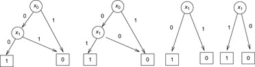
For evaluating the represented function for a given input, a path is traced from the root node to one of the sinks, quite similar to the way Decision Trees are used. What distinguishes BDDs from Decision Trees is the use of two reduction rules, detecting unnecessary variable tests and isomorphisms in subgraphs, leading to a unique representation that is polynomial in the length of the bit strings for many interesting functions.
Definition 7.2
(Reduced and Ordered BDD) A reduced and ordered BDD is a BDD where on each path a fixed ordering of variables is preserved (ordered BDD) and where nodes with identical successors are omitted and isomorphic sub-BDDs are merged (reduced BDD).
Figure 7.2 illustrates the application of these two rules. An unreduced and a reduced BDD for the goal state of the example problem is shown in Figure 7.3.

 |
| Figure 7.3 |
Throughout this chapter we write BDDs, although we always mean reduced and ordered BDDs. The reason that the reduced representation is unique is that each node in a BDD represents an essential subfunction. The uniqueness of BDD representation of a Boolean function implies that the satisfiability test is available in  time. (If the BDD merely consists of a 0-sink, then it is unsatisfiable, otherwise it is satisfiable.) This is a clear benefit to a general satisfiability test of Boolean formulas, which by the virtue of Cook's theorem is an NP-hard problem. Some other operations on BDDs are:
SAT-Count Input: BDD  . Output:
  . Running time:
  . Description: The algorithm considers a topological ordering of the nodes in the BDD. It propagates the number of possible assignments at each internal node bottom-up. Application: For state space search, the operation determines the number of explicit states that are represented by a BDD. In AI literature, this operation is also referred to as model counting.
Synthesis Input: BDDs  and
and  , operator
  . Output: BDD for
  . Running time:
  . Description: The implementation traverses both input graphs in parallel and generates the result by merging matching subtrees bottom-up. The synchronization between the two parallel depth-first searches is the variable ordering. If the index in the first BDD is larger than in the other, it has to wait. As the traversal is depth-first, the bottom-up construction is organized postorder. For returning a reduced BDD the application of both reduction rules is included in the parallel traversal. Application: For state space search, synthesis is the main operation to construct unions and intersections of state sets.
Negation Input: BDD  . Output: BDD for
  . Running time:
  . Description: The algorithm simply exchanges the labels of the sinks. Analogous to the satisfiability test it assumes the sinks are accessible in constant time. Application: In state space search, negation is needed to remove a state set, as set subtraction is realized via a combination of a conjunction and a negation.
Substitution-by-Constant Input: BDD  , variable
  , and constant
  . Output: BDD
  . Running time:
  . Description: The algorithm sets all
  successors of
  to the zero sink (followed by BDD reduction). Application: In state space search, variants for substitution-by-constant are needed to reconstruct the solution path.
Relational Product Input: BDDs  and
and  , variable
  . Output: BDD
  (or
(or  ). Running time:
  . Description: The basic algorithm applies the synthesis algorithm for
  ,
,  and
and  (or
(or  and
and  , and
, and  ). Algorithm 7.11 (see Exercises) shows how to integrate quantification with the additional operator
  (or →). Application: In state space search, the relational is used when computing the images and preimages of a state set.
Substitution-by-Variable Input: BDD  , variable
  and
and  (f does not depend on
  ). Output: BDD
  . Running time:
  . Description: The function
  can be written as
  , so that a substitution by variable is a relational product. (If
  follows
  in the variable ordering the algorithm simply relabels all
  nodes with
  in
in  time.) Application: In state space search, substitution-by-variable is needed to change the variable labels.
The variable ordering has a huge influence on the size (the space complexity in terms of the number of nodes to be stored) of a BDD. For example, the function  has linear size (
 nodes) if the ordering matches the permutation
  , and exponential size (
 nodes) if the ordering matches the permutation
  . Unfortunately, the problem of finding the best ordering (the one that minimized the size of the BDD) for a given function f is NP-hard. The worst case are functions that have exponential size for all orderings (see Exercises) and, therefore, do not suggest the use of BDDs.
For transition relations, the variable ordering is also important. The standard variable ordering simply appends the variables according to the binary representation of a state; for example,  . The interleaved variable ordering alternates x and
  variables; for example,
  .
.
The BDD for the transition relation  for a noninterleaved variable ordering is shown in Figure 7.4. (Drawing the BDD for the interleaved ordering is left as an exercise.)
 |
| Figure 7.4 |
There are many different possibilities to come up with an encoding of states for a problem and a suitable ordering among the state variables. The more obvious ones often waste a lot of space. So it is worthwhile to spend efforts in finding a good ordering. Many applications select orderings based upon an approximate analysis of available input information. One approach is a conflict analysis, which determines how strong a state variable assignment depends on another. Variables that are dependent of each other appear as close as possible in the variable encoding.
Alternatively, advanced variable ordering techniques have been developed, such as the sifting algorithm. It is roughly characterized as follows. Because a BDD has to respect the variable ordering on each path, it is possible to partition it according to levels of nodes with the same variable index. Let  be the level of nodes with variable index i,
  . The sifting algorithm repeatedly seaks a better position in the variable ordering for a variable (or an entire group of variables) by moving it up (or down) in the current order, and evaluating the result by measuring the resulting BDD size. In fact, variables
  are selected, for which the levels
  in the BDDs are at their widest; that is, for which
  is maximal. Interestingly, the reordering technique can be invoked dynamically during the course of computations.
Performing arithmetics is essential for many BDD-based algorithms. In the following we illustrate how to perform addition with finite-domain variables using BDDs (multiplication is dealt with analogously). Since most BDD packages support finite-domain variables, we abstract from the binary representation. Because it is not difficult to shift a domain from [min, max] to [0, max − min], without loss of generality, in the following we assume all variable domains start with value 0 and end with value max.
First, the BDD  that encodes the binary relation
  can be constructed by enumerating all possible assignments of the form
  ,
,  ,
, assuming that the binary relation
  , written as
  , is provided by the underlying BDD package.
BDD  represents the ternary relation
  . For the construction, we might enumerate all possible assignments to the variables a, b, and c. For large domains, however, the following recursive computation should be preferred:
 Hence, Add is the result of a fixpoint computation. Starting with the base case
  , which unifies all cases in which the according relation is true, the closure of Add is computed by applying the second part of the equation until the BDD representation no longer changes. The pseudo code is shown in Algorithm 7.1. To allow multiple quantification, in each iteration the sets of variables (for the parameters b and c) are swapped (denoted by
  ). The BDDs From and New denote the same set, but are kept as separate concepts: one is used for termination detecting and the other for initiating the next iteration.

7.3. Computing the Image for a State Set
What have we achieved so far? We are able to reformulate the initial and final states in a state space problem as BDDs. As an end in itself, this does not help much. We are interested in a sequence of actions that transforms an initial state into one that satisfies the goal.
By conjoining the transition relation with a formula describing a set of states, and quantifying the predecessor variables, we compute the representation of all states that can be reached in one step from some state in the input set. This is the relational product operator. Hence, what we are really interested in is the image of a state set S with respect to a transition relation Trans, which is equal to applying the operation where
where  denotes the characteristic function of set S. The result is a characteristic function of all states reachable from the states in S in one step. For the running example, the image of the state set
  represented by
  is given by
 and represents the state set
  .
.
More generally, the relational product of a vector of Boolean variables x and two Boolean functions f and g combines quantification and conjunction in one step and is defined as  . Since existential quantification of a Boolean variable
  in the Boolean function f is equal to
  , the quantification of the entire vector x results in a sequence of subproblem disjunctions. Although computing the relational product (for the entire vector) is NP-hard in general, specialized algorithms have been developed leading to an efficient determination of the image for many practical applications.
7.4. Symbolic Blind Search
First, we turn to undirected search algorithms that originate in symbolic model checking.
7.4.1. Symbolic Breadth-First Tree Search
In a symbolic variant of BFS we determine the set of states  reachable from the initial state s in i steps. The search is initialized with
  . The following image equation determines
  given both
  and the transition relation Trans:
 Informally, a state
  belongs to
  if it has a predecessor x in the set
  and there exists an operator that transforms x into
  . Note that on the right side of the equation
  depends on x, compared to
  on the left side. Thus, it is necessary to substitute
  with x in
  for the next iteration. There is no need to reorder or reduce, because the substitution can be done by a textual replacement of the node labels in the BDD.
To terminate the search we test whether or not a state is represented in the intersection of the set  and the set of goal states T. Since we enumerated the sets
  , the first iteration index i with
  denotes the optimal solution length.
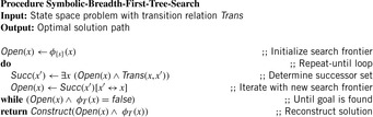
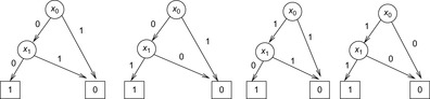
Let Open be the representation of the search frontier and let Succ be the BDD for the set of successors. Then the algorithm symbolic breadth-first tree search can be realized as the pseudo code Algorithm 7.2 suggests. (For the sake of simplicity, in this and upcoming algorithms we generally assume that the start state is not a goal.) It leads to three iterations for the example problem (see Fig. 7.5). We start with the initial state represented by a BDD of two inner nodes for the function  . After the first iteration we obtain a BDD representing the function
  . The next iteration leads to a BDD of one internal node for
  , and the last iteration results in a BDD for
  that contains the goal state. The corresponding content of the Open list is made explicit in Table 7.3.
| Step | State Set | Binary Codes | Boolean Formula |
|---|---|---|---|
| 0 | |||
| 1 | |||
| 2 | |||
| 3 |
Theorem 7.1
(Optimality and Complexity of Symbolic Breadth-First Tree Search) The solution returned by symbolic breadth-first tree search has the minimum number of steps while applying the same number of images.
Proof
The algorithm generates every reachable state in the search tree with repeated image operations in a breadth-first manner, such that the first goal state encountered has optimal depth.
By keeping track of the intermediate BDDs, a legal sequence of states linking the initial state to a goal state can be extracted, which in turn can be used to find a corresponding sequence of actions. The goal state is on the optimal path. A state in an optimal path that comes before the detected goal state must be contained in the previous BFS level. We, therefore, intersect the predecessors of the goal state with that level. All states that are in the intersection are reachable in an optimal number of steps and reach the goal with an optimal number of steps, so any of these states can be chosen to continue solution reconstruction until the initial state is found.
If all previous BFS levels remain in main memory, sequential solution reconstruction is sufficient. If levels are eliminated (as in frontier search; see Ch. 6), a solution reconstruction from BFS levels flushed to disk is recommended.
7.4.2. Symbolic Breadth-First Search
The introduction of a list Closed containing all states ever expanded is the common approach in the explicit-state exploration to avoid duplicates. In symbolic breadth-first search (see Alg. 7.3) this technique is realized through the refinement  for the successor state set Succ. The operation is called forward or frontier set simplification. One additional advantage is that the algorithm terminates in case no solution exists.
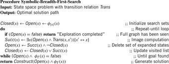
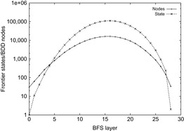
The BDDs for exploring the Sliding-Token Puzzle are shown in Figure 7.6 with formula representations listed in Table 7.4. For bigger examples, memory savings by applying the functional state set representation in the BDD are expected to grow. Figure 7.7 shows a typical behavior.
| Step | State Set | Binary Codes | Boolean Formula |
|---|---|---|---|
| 0 | |||
| 1 | |||
| 2 | |||
| 3 |
Theorem 7.2
(Optimality and Complexity of Symbolic BFS) The solution returned by symbolic BFS has the minimum number of steps. The number of images is equal to the solution length. It stops if a problem obeys no solution.
Proof
The algorithm expands each possible node in the problem graph with repeated image operations at most once, such that the first goal state encountered has optimal depth. If no goal is returned the entire reachable search space has been explored.
In Chapter 6, we saw that for some problem classes like undirected or acyclic graphs, duplicate elimination can be limited from all to a reduced number of BFS levels. In undirected search spaces, it is also possible to apply frontier search (see Ch. 6). In the (n2−1)-Puzzle for each BFS level, all permutations (vectors) have the same parity (minimum transpositions needed to transform the state vector into the identity modulo 2, either even or odd). This implies that states in odd depths cannot reappear in an even depth and vice versa. As a consequence, only BFS level  has to be subtracted from BFS level i to remove all duplicates from the search.
7.4.3. Symbolic Pattern Databases
We have seen that the main limitation for applying pattern databases in search practice is the restricted amount of (main) memory and that the objective in symbolic search is to represent large sets of states with BDD nodes.
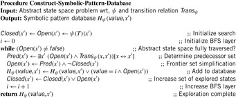
Symbolic pattern databases are pattern databases that have been constructed symbolically for later use either in symbolic or explicit heuristic search. It is based on the advantage of the fact that Trans has been defined as a relation. In backward breadth-first search we start with the goal set  and iterate until we encounter the start state. We then successively compute the preimage according to the formula
 Each state set is efficiently represented by a corresponding characteristic function. Different to the posterior compression of the state set, the construction itself works on the compressed representation, allowing much larger databases to be constructed.
For symbolic pattern database construction, backward symbolic BFS is used. For an abstraction function  the symbolic pattern database
  is initialized with the projected goal set
  and, as long as there are newly encountered states, we take the current list of frontier nodes and generate the predecessor list with respect to the abstracted transition relation
  . Then we attach the current BFS level to the new states, merge them with the set of already reached state states, and iterate. In Algorithm 7.4Closed is the set of visited states for backward search, Open is the current abstract search frontier, and Pred is the set of abstract predecessor states.
Note that in addition to the capability to represent large sets of states in the exploration, symbolic pattern databases have one further advantage to explicit ones: fast initialization. In the definition of most problems the goal is not given as a collection of states but as a formula to be satisfied. In explicit-pattern database construction all goal states have to be generated and inserted into the backward exploration queue, but for the symbolic construction, initialization is immediate by building the BDD for the goal formula.
If we consider the example of the Thirty-Five-Puzzle with x tiles in the pattern, the abstract state space consists of  states. A perfect hash table for the Thirty-Five-Puzzle has space requirements of 43.14 megabytes (
 ), 1.3 gigabytes (
 ), and 39.1 gigabytes (
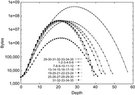
 ). The memory required for storing symbolic pattern databases is plotted in Figure 7.8, suggesting a moderate but noticeable reduction with regard to the corresponding explicit construction; that is, the seven-tile pattern database requires 6.6 gigabytes of RAM. In other domains, it has been observed that the savings of symbolic pattern databases scale to several orders of magnitude.
 |
| Figure 7.8 |
Another key performance of symbolic pattern databases is a fast construction time. Given that pattern construction is an exploration in abstract state spaces, in some cases the search performance corresponds to billions of states being generated in a second.
7.4.4. Cost-Optimal Symbolic Breadth-First Search
Symbolic BFS finds the optimal solution in the number of solution steps. BDDs are also capable of space-efficiently optimizing a cost function f over the problem space. In this section, we do not make any specific assumption about f(e.g., being monotone or being composed of g or h), except that f operates on variables of finite domains. The problem has become prominent in the area of (oversubscribed) action planning, where a cost function encodes and accumulates the desire for the satisfaction of soft constraints on planning goals, which has to be maximized. As an example, consider that in addition to an ordinary goal description, we prefer certain blocks in Blocksworld to be placed on the table. For the sake of simplicity, we restrict ourselves to minimization problems. This implies that we want to find the path to a goal node in T that has the smallest f-value.
To compute a BDD  for the cost function
  over a set of finite-domain state variables
  with
with  , we first compute the minimum and maximum values that f can take. This defines the range
  that has to be encoded in binary. For example, if f is a linear function
  with
with  ,
,  then
then  and
and  .
.
To construct  we build sub-BDD
  with value representing
  ,
,  , and combine the intermediate results to the relation
  using the relation Add. As the
  are finite the relation
  can be computed by using
  (
( times) or by adapting the ternary relation Mult. This shows that all operations to construct F can be realized using finite-domain arithmetics on BDDs. Actually, there is a direct option for constructing the BDD of a linear function directly from the coefficients in
  time and space.
Algorithm 7.5 displays the pseudo code for symbolic BFS incrementally improving an upper bound U on the solution cost. The algorithm applies symbolic BFS until the entire search space has been traversed and stores the current best solution. As before, state sets are represented in the form of BDDs. Additionally, the search frontier is reduced to those states that have a cost value of at most U. In case an intersection with the goal is found, the breadth-first exploration is suspended to construct a solution with the smallest f-value for states in the intersection. The cost gives a new upper bound U denoting the quality of the current best solution minus 1. After the minimal cost solution has been found, the breadth-first exploration is resumed.
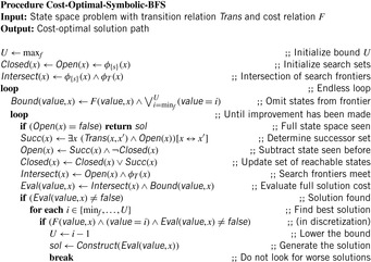
Theorem 7.3
Proof
The algorithm applies duplicate detection and traverses the entire state space. It generates each possible state exactly once. Eventually, the state with the minimal f-value will be found. Only those goal states are abandoned from the cost evaluation that have an f-value larger than or equal to the current best solution. The exploration terminates if all BFS levels have been generated. Thus, the number of images matches the maximum BFS-level.
7.4.5. Symbolic Shortest Path Search
Before turning to the symbolic algorithms for directed search, we take a closer look at the bucket implementation of Dijkstra's Single-Source Shortest Path algorithm for solving search problems with action costs.
Finite action costs are a natural search concept. In many applications, costs can only be positive integers (sometimes for fractional values it is also possible and beneficial to achieve this by rescaling). Since BDDs allow sets of states to be represented efficiently, the priority queue of a search problem with integer-valued cost function can be partitioned to a list of buckets. We assume that the highest action cost and f-value are bounded by some constant.
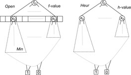
The priority queue of a search problem with an integer-valued cost function can be implemented as a set of pairs, of which the first component is the f-value and the second component is the x-value. In a functional representation pairs correspond to satisfying paths in a BDD  . The variables for the encoding of f can be assigned smaller indices than the variables encoding x, since, aside from the potential to generate smaller BDDs, this allows an intuitive understanding of the BDDs and its association with the priority queue. Figure 7.11 (left) illustrates the representation of the priority queue in the form of BDDs.
The symbolic version of Dijkstra's algorithm can be implemented as shown in Algorithm 7.6. For the sake of simplicity, the algorithm has no Closed list, so that it can contain identical states with different f-values. (As with symbolic breadth-first tree search, duplicate elimination is not difficult to add, but may induce additional complexity to the BDD.)
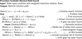
The working of the algorithm is as follows. The BDD Open is set to the representation of the start state with f-value 0. Unless we establish a goal state, in each iteration we extract all states with minimum f-value fmin. The easiest option to find the next value of fmin is to test all internal values f starting from the last value of fmin for intersection with Open. A more efficient option is to exploit the BDD structure in case the f-variables are encoded on top of the BDD.
Given fmin, next we determine the successor set and update the priority queue. The BDD Min of all states in the priority queue with value fmin is extracted, resulting in the BDD Rest of the remaining set of states. If no goal state is found, the variables in Min (the transition relation  is applied to) determine the BDD for the set of successor states. To calculate
  and to attach new f-values to this set, we store the old f-value fmin. Finally, the BDD Open for the next iteration is obtained by the disjunction of the successor set with the remaining queue.
Theorem 7.4
(Optimality of Symbolic Shortest Path Search) For action weights  , the solution computed by the symbolic shortest path search algorithm is optimal.
Proof
The algorithm mimics the Single-Source Shortest Path algorithm of Dijkstra on a 1-Level Bucket structure (see Ch. 3). Eventually, the state with the minimum f-value is found. As f is monotonically increasing, the first goal reached has optimal cost.
Theorem 7.5
(Complexity of Symbolic Shortest Path Search) For positive transition weights  , the number of iterations (BDD images) in the symbolic shortest path search algorithm is
  , where
  is the optimal solution cost.
Proof
The number of iterations (BDD images) is dependent on the number of buckets that are considered during the exploration. Since the edge weight is a positive integer, we have at most  iterations, where
  is the optimal solution cost.
7.5. Limits and Possibilities of BDDs
To uncover the causes for good and bad BDD performance we aim at lower and upper bounds for BDD growth in various domains.
7.5.1. Exponential Lower Bound
We first consider permutation games on  , such as the (n2−1)-Puzzle, where
  . The characteristic function
  of all permutations on
  has
has  binary state variables and evaluates to true, if every block of
  variables corresponds to the binary representation of an integer and every satisfying path of N integers is a permutation.
It is known that the BDD for  needs more than
  BDD nodes for any variable ordering. This suggests that permutation games are hard for BDD exploration.
7.5.2. Polynomial Upper Bound
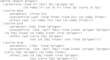
In other state spaces, we obtain an exponential gain using BDDs. Let us consider a simple planning domain, called Gripper. The domain description is provided in Figure 7.9. There is one robot to transport  balls from one room A to another room B. The robot has two grippers to pick up and put down a ball.
It is not difficult to observe that the state space grows exponentially. Since we have  , the number of all states with k balls in one room is
  . The precise number of all reachable states is
  , where
  corresponds to the number of all states with no ball in a gripper.
The basic observation is that all states with an even number of balls in each room (apart from the two states with all balls in the same room and the robot in the other one) are part of an optimal plan. For larger values of n, therefore, heuristic search planners even with a constant error of only 1 are doomed to fail.
The robot's cycle for delivering two balls from one room to the other in any optimal plan has length six (picking up the two balls, moving from one room to the other, putting down the two balls, and moving back), such that every sixth BFS layer contains the states on an optimal plan with no ball in a gripper. Yet there are still exponentially many of these states, namely,  .
.
Theorem 7.6
(Exponential Representation Gap for Gripper) There is a binary state encoding and an associated variable ordering, in which the BDD size for the characteristic function of the states on any optimal path in the breadth-first exploration of Gripper is polynomial in n.
Proof
To encode states in Gripper,  bits are required: one for the location of the robot,
  for each of the grippers to denote which ball it currently carries, and 2 for the location of each ball. According to BFS, we divide the set of states on an optimal path into levels l,
  . If both grippers are empty and the robot is in the right room, all possible states with
  balls in the right room have to be represented, which is available using
  BDD nodes. See Figure 7.10 for a BDD representing at least b balls in room B. The BDD for representing exactly b balls in room B is a slight extension and includes an additional tail of
  nodes (see Exercises). The number of choices with one or two balls in the gripper that are addressed in the
  variables is bounded by
  , such that intermediate levels may lead to at most a quadratic growth. Hence, each layer restricted to the states on the optimal plan contains less than
  BDD nodes in total. Accumulating the numbers along the path, of which the size is linear in n, we arrive at less than
  BDD nodes needed for the entire exploration.
We next look at the Sokoban domain, where we observe another exponential gap between explicit-state and symbolic representation.
As we have  , the number of all reachable states is clearly exponential.
Theorem 7.7
(Exponential Representation Gap for Sokoban) If all  configurations with k balls in a maze of n cells in Sokoban are reachable, there is a binary state encoding and an associated variable ordering, in which the BDD size for the characteristic function of all reachable states in Sokoban is polynomial in n.
Proof
To encode states in Sokoban,  bits are required; that is, 2 bits for each cell (stone/player/none). If we were to omit the player, we would observe a similar pattern to the one in Figure 7.10, where the left branch would denote an empty cell and the right branch a stone, leaving a BDD of
  nodes. Integrating the player results in a second BDD of size
  with links from the first to the second. Therefore, the complexity for representing all reachable Sokoban positions requires a polynomial number of BDD nodes.
7.6. Symbolic Heuristic Search
We have seen that in heuristic search, with every state in the search space we associate a lower-bound estimate h on the optimal solutions cost. Further, at least for consistent heuristics by reweighting the edges, the algorithm of A* reduces to Dijkstra's algorithm. The rank of a node is the combined value  of the generating path length g and the estimate h.
7.6.1. Symbolic A*
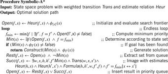
A* can be cast as a variant of Dijkstra's algorithm with (consistent) heuristics. Subsequently, in the symbolic version of A* the relational product algorithm determines all successors of the set of states with minimum f-value in one image operation. It remains to determine their f-values. For the dequeued state u we have  . Since we can access the f-value, but usually not the g-value, the new f-value of a successor v has to be calculated in the following way:
The estimator Heur can be seen as a relation of tuples  , which is true if and only if the heuristic value of the states represented by x is equal to a number represented by value. We assume that the heuristic relation Heur can be represented as a BDD for the entire problem space (see Fig. 7.11, right).
There are different options to determine Heur. One approach tries to implement the function directly from its specification (see Exercises for an implementation of the Manhattan distance heuristic in the (n2−1)-Puzzle). Another option simulates explicit-pattern databases (as introduced in Ch. 4) that Heur is the outcome of a symbolic backward BFS or Dijkstra exploration in abstract space. The implementation of A* is shown in Algorithm 7.7. Since all successor states are reinserted in the queue we expand the search tree in best-first manner.
The BDD arithmetics for computing the relation  based on the old and new heuristic values (h and
  , respectively) and the old and new costs (
 and f, respectively) are involved:
 Optimality and completeness of A* are inherited from the fact that given an admissible heuristic, explicit-state A* will find an optimal solution.
By pushing variables inside the calculation of Succ can be simplified to
Let us consider our Sliding-Token Puzzle example once again. The BDD for the estimate h is depicted in Figure 7.12, where the estimate is set to 1 for states 0 and 1, and set to 0 for states 3 and 4.

The minimum f-value is 1. Assuming that  will be bounded by 4 we need only two variables,
  and
and  , to encode f(by adding 1 to the binary encoded value).
After the initialization step, the priority queue Open is filled with the initial state represented by the term  . The h-value is 1 and so is the initial f-value (represented by
  ). There is only one successor to the initial state, namely
  , which has an h-value of 1 and, therefore, an f-value of
  . Applying Trans to the resulting BDD-we obtain the combined characteristic function of the states with index 0 and 2. Their h-values differ by 1. Therefore, the term
  is assigned to an f-value of
  and
and  is assigned to
  (the status of the priority queue is depicted in Fig. 7.13, left). In the next iteration we extract
  with value 2 and find the successor set, which in this case consists of
  and
and  . By combining the characteristic function
  with the estimate h we split the BDD of
  into two parts, since
  relates to an h-value 0, whereas
  relates to 1 (the resulting priority queue is shown in Fig. 7.13, right). Since Min now has a nonempty intersection with the characteristic function of the goal, we have found a solution. The represented state sets and their binary encoding are shown in Table 7.5. The minimum f-value is 3, as expected.
 |
| Figure 7.13 The priority queue Open after two (left) and after three (right) exploration steps in symbolic A* search for the Sliding-Token Puzzle example. Variables encoding the f-value are encoded by |
To exemplify the effectiveness of the approach, we consider the Sokoban problem. To compute the step-optimal solution for the problem of Figure 1.14 A* has been invoked with a heuristic that counts the number of balls not on a goal position. Symbolic BFS finds the optimal solution with a peak BDD of 250,000 nodes (representing 61 million states) in 230 iterations, and A* leads to 419 iterations and to a peak BDD of 68,000 nodes (representing 4.3 million states).

7.6.2. Bucket Implementation
Symbolic A* applies to unweighted graphs or graphs with integer action costs. Its functional implementation can be applied even to infinite state spaces by using more expressive representation formalisms than BDDs (like automata for state sets induced by linear constraints over the integers).
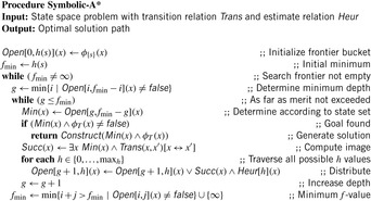
For small values of C and a maximal h-value  , it is possible to avoid arithmetic computations with BDDs. We assume unit action costs and that the heuristic relation is partitioned into
  , with
We use a two-dimensional bucket layout for the BDDs as shown in Figure 7.14. The advantages are two-fold. First, the state sets to be expanded next are generally smaller, and the hope is that the BDD representation is as well. Second, given the bucket by which a state set is addressed, each state set already has both the g-value and the h-value attached to it, and the arithmetic computations that were needed to compute the f-values for the set of successors are no longer needed. The refined pseudo-code implementation for A* is shown in Algorithm 7.8.
Theorem 7.8
(Optimality of Symbolic A*) Given a unit cost problem graph and a consistent heuristic, the solution cost computed by A* is optimal.
Proof
The algorithm mimics the execution of the reweighted version of Dijkstra's algorithm on a 1-Level Bucket structure. Eventually, the state of the minimum f-value will be encountered. Since the reweighted action costs are nonnegative, f is monotonic increasing. Hence, the first encountered goal state has optimal cost.
For an optimal heuristic, one that estimates the shortest path distance exactly, we have at most  iterations in A*. On the other hand, if the heuristic is equivalent to the zero function (breadth-first search), we need
  iterations, too.
Theorem 7.9
(Complexity Symbolic A*) Given a unit cost problem graph and a consistent heuristic the worst-case number of iterations (BDD operations) in A* is  , with
  being the optimal solution length.
Proof
There are at most  different h-values and at most
  different g-values that are encountered during the search process. Consequently, for each period between two successive increases of the minimum f-value, we have at most
  iterations. Consider Figure 7.14, in which the g-values are plotted with respect to the h-value, such that nodes with the same g-value and h-value appear on the diagonals
  . Each bucket is expanded at most once. All iterations (marked by a circle) are located on or below the
  -diagonal, so that
  is an upper bound on the number of iterations.
For heuristics that are not consistent, we cannot terminate at the first goal that we encounter (see Exercises). One solution is to constrain the g-value to be less than the current best solution cost value f.
7.6.3. Symbolic Best-First Search
A variant of the symbolic execution of A*, called symbolic greedy best-first search, is obtained by ordering the priority queue Open only according to the h-values. In this case the calculation of the successor relation simplifies to  (Min
(Min 


 as shown in the pseudo code of Algorithm 7.9. The old f-values are ignored.

Unfortunately, even for admissible heuristics the algorithm is not optimal. The hope is that in huge problem spaces the estimate is good enough to lead the solver into a promising goal direction. Therefore, especially inadmissible heuristics can support this aim.
On solution paths the heuristic values eventually decrease. Hence, symbolic greedy best-first search profits from the fact that the most promising states are in the front of the priority queue and are explored first. This compares to A* in which the f-value on the solution paths eventually increases.
In between A* and greedy best-first search, there are different best-first algorithms. For example, scaling the heuristic estimate similar to the weighted A* algorithm is as follows. If  denotes the heuristic relation a weight factor
  can be introduced by constructing
  .
.
7.6.4. Symbolic Breadth-First Branch-and-Bound
Even for symbolic search, memory consumption remains a critical resource for a successful exploration. This motivates a breadth-first instead of a best-first traversal of the search space (as illustrated in the context of breadth-first heuristic search in Ch. 6).
Symbolic breadth-first branch-and-bound generates the search tree in breadth-first instead of best-first order. The core search routine is invoked with a bound U on the optimal solution length, which can be provided by the user or automatically inferred by nonoptimal search algorithms like beam search. Using the bound U, buckets are neglected from the search if their  -value is larger than U.
Algorithm 7.10 shows an implementation of this strategy for symbolic search. The algorithm traverses the matrix of buckets  with increasing depth g, where each breadth-first level is pruned by the bound U.
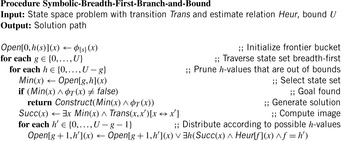
In the exposition of the strategy again we assume a unit cost problem graph in the input and the implementation of a construction algorithm for extracting the solution path (e.g., using a divide-and-conquer approach by keeping an additional relay layer in main memory). For the sake of clarity, we have also omitted symbolic duplicate elimination.
If the graph has been fully explored without generating any solution, we know that there is no solution of length  . Hence, breadth-first branch-and-bound returns the optimal solution, if the value U is chosen minimally in providing a solution. As a consequence, breadth-first iterative-deepening A* operating with an increasing threshold U is optimal.
If the bound to solution length U provided to the algorithm is minimal, we can also expect time and memory savings with regard to symbolic A* search, since states that exceed the given bound are neither generated nor stored. If the bound, however, is not optimal, the iterative-deepening algorithm may explore more states than symbolic A*, but retain the advantage in memory.
Theorem 7.10
(Complexity of Symbolic Breadth-First Branch-and-Bound) Provided with the optimal cost threshold  , symbolic breadth-first branch-and-bound (without duplicate elimination) computes the optimal solution in at most
  image operations.
Proof
If  , the buckets considered with a
  -value smaller than or equal to
  are the same as in A*, this algorithm also considers the buckets on the diagonals with rising g-value. Subsequently, we obtain the same number of images.
In search practice, the algorithm shows some memory advantages. In an instance of the Fifteen-Puzzle for which explicit-state A* consumes 1.17 gigabytes of main memory, and breadth-first heuristic search consumes 732 megabytes, A* consumes 820 megabytes, and symbolic heuristic (branch-and-bound) search consumes 387 megabytes.
As said, finding the optimal cost threshold can be involved and the iterative computation is more time consuming than applying A* search. Moreover, A* may also be implemented with a delayed expansion strategy. Consider the case of the (n2−1)-Puzzle with Manhattan Distance heuristic, where each bucket is expanded twice for each f-value. In the first pass, only the successors on the active diagonal are generated, leaving out the generation of the successors on the  -diagonal. In the second pass, the remaining successors on the
  -diagonal are generated. We can avoid computing the estimate twice, since all successor states that do not belong to the bucket
  belong to the bucket
  . In the second pass we can therefore generate all successors and subtract bucket
  from the result. The complexity of this strategy decreases from exploring
  edges to exploring
  . Hence, expanding each state twice compensates for a large number of generated nodes above the
  -diagonal that are not stored in the first pass.
7.7. * Refinements
Besides forward set simplification there are several improvement tricks that can be played to improve the performance of the BDD exploration.
7.7.1. Improving the BDD Size
Any set smaller than the successor set Succ and larger than the successor set Succ with simplified set Closed of all states reached already will be a valid choice for the frontier Open in the next iteration.
In the Shannon-expansion of a Boolean function f with respect to another function g, defined by  , this determines
  and
and  at the position
  with
with  and
and  . However, if
  or
or  we have some flexibility. Therefore, we may choose a set that minimizes the BDD representation instead of minimizing the set of represented states. This is the idea of the restrict operator
  , which itself is a refinement to the constrain operator
  . Since both operators are dependent of the ordering, we assume the ordering
  to be the trivial permutation. We define the distance
  of two Boolean vectors a and b of length n by the sum of
  for
for  . The constrain operator
  of two Boolean functions f and g evaluated at a vector a is then determined as
  if
if  , and as
  if
if  ,
,  , and
, and  is minimum. The restrict operator
  now incorporates the fact that for the function
  we have
  . Without going into more details we denote that such optimizing operators are available in several BDD packages.
7.7.2. Partitioning
The image Succ of the state set Open with respect to the transition relation Trans has been computed as  . In this image,
  is assumed to be monolithic; that is, represented as one big relation. For several domains, constructing such a transition relation prior to the search consumes huge amounts of the available computational resources. Fortunately, it is not required to build Trans explicitly. Hence, we can keep it partitioned, keeping in mind that
  for each individual transition relation
  and each action
  .
.
The image now reads as Therefore, the monolithic construction of Trans can be bypassed. The execution sequence of the disjunction has an effect on the overall running time. The recommended implementation organizes this partitioned image in the form of a balanced tree.
For heuristic functions that can be computed incrementally in a small integer range, there is the choice to group state pairs  that have a common heuristic difference d. This leads to a limited set of relations
  . One example is the Manhattan distance heuristic with
  for all successors v of u. For this case, we split the possible transition
  into two parts
  and
and  . The successors of a frontier bucket Open with coordinates g and h can now be inserted either into bucket
  or into
  .
.
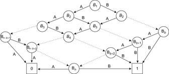
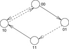
Such incremental computations are exploited in images via branching partitions. The abstracted transition expressions are partitioned according to which variables they modify. Take, for example, the set of transitions  ,
,  , and
, and  that modify variable
  , as well as
  and
and  that modify variable
  . Figure 7.15 depicts the transition system with solid arrows for one and dashed arrows for the other branching partition.
7.8. Symbolic Algorithms for Explicit Graphs
Symbolic search approaches are also under theoretical and empirical investigation for classic graph algorithms, like Topological Sorting, Strongly Connected Component, Single-Source Shortest Path, All-Pairs Shortest Path, and Maximum Flow. The difference from the earlier implicit setting is that the graph is now supposed to be an input of the algorithms. In other words, we are given a graph  with source
  represented in the form of a Boolean function or BDD
  , such that
  if and only if
  and
and  for all u and v.
For the encoding of the  nodes, a bit string of length
  is used, so that edges are represented by a relation with 2k variables. To perform an equality check
  in linear time an interleaved ordering
  is preferred to a sequential ordering
  .
.
Since the maximum accumulated weight on a path can be  , the fixed size of the encoding of the weight function should be of size
  . It is well known that the BDD size for a Boolean function on l variables is bounded by
  nodes, since given the reduced structure, the deepest levels have to converge to the two sinks. Using a binary encoding for V and weights in nd we have that the worst-case size of the BDD Graph is of order
  , and the hope is that many structured graphs have a sublinear BDD with size
  . Since we cannot expect a gain for general graphs in the worst case, symbolic versions for explicit-graph algorithms are designed for sublinear runtime on special graphs and acceptable average-case behavior.
The symbolic Single-Source Shortest Path algorithm maintains distance function  in the form of a BDD Dist such that
  if and only if
  . As we have discussed before, Dijkstra's algorithm considers nodes in the set Closed that already have a shortest path, selects nodes
  with minimum
  , and adds u to Closed. Then it updates f for neighbors v of u according to
  . With BDD operations and n being the number of nodes in the graph, one iteration can be performed with
  BDD operations. Having at most
  iterations, we have at most
  BDD operations in total.
For the Bellman-Ford algorithm we relax every node  with
with  followed by an update of
  . This can be achieved using a BDD representation for Relax on the variables for u, v, and d that evaluates to true if
  . In other words, the relation Relax is defined by
 In total, we have
  BDD operations. The observation is that Dijkstra's algorithm leads to many fast operations, since the symbolic sets are fairly structured, whereas the algorithm of Bellman and Ford relaxes edges in parallel, which leads to fewer operations, but each operation is considerably slow. Experiments on random graphs show that even though Dijkstra needs space almost linear in the size of the BDD representation of the input graph, Bellman-Ford is usually faster.
7.9. Summary
Symbolic search algorithms use a functional representation to express large but finite sets of states based on a finite-domain state encoding. We have chosen binary decision diagrams (BDDs) for the space-efficient unique representation of these functions. Other representations for Boolean functions (e.g., Algebraic Decision Diagrams (ADDs), And Inverter Graphs, and Decomposable Negational Normal Forms (DNNFs)) do not change the exploration algorithms. Other symbolic data structures (e.g., Presburger automata and difference bound matrices) can cover infinite state sets, but follow similar algorithmic principles.
The advantages of symbolic search with BDDs for representing state sets include
• The exploitation of similarities within the state vector (due to path sharing in the graph structure of the BDD).
• The observation that a polynomially sized BDD may contain exponentially many paths.
• The uniqueness of the representation (which avoids any form of duplicate detection within the represented set).
• The functional1 exploration of the state space (which avoids an intermediate uncompressed representation during the exploration).
During the exploration, a minimized binary variable encoding (e.g.,  for
for  ) outperforms a unary encoding of predicates (e.g.,
  for
for  ). Using an appropriate relevance measure on the dependency of variables, good orderings can be obtained that lead to smaller BDDs. As an immediate consequence, precondition and effect variables should be interleaved. Permutation games are likely to be hard for BDDs, whereas games that are based on selecting indistinguishable objects appear to be easier.
Symbolic search relies on a transition relation that takes twice the number of state variables. The relation features both forward and backward search and can be extended to include action costs. If possible, the transition relation should be kept partitioned to keep the most expensive image operation tractable for larger problems. As enumerating all problem graph edges is out of reach for an implicit graph search, we have introduced partitions by individual actions (disjunctive partitioning), by abstract distance values (pattern database partitioning), by hash differences (branching partitioning), and by discrete action costs (cost value partitioning). Using a discretization into  buckets, BDD arithmetics can be avoided. Duplicate detection with respect to previous exploration sets is not necessarily an advantage, as it may complicate the BDD representation, but as a trade-off, we can detect a nonsolvable search problem due to a complete exploration. Even though it is difficult to formalize by the series of subproblem disjunctions, the number of represented states seems to have some influence on the hardness of computing the image of a state set. The number of previous levels that need to be maintained in the RAM to preserve full duplicate detection has been introduced in previous chapters (e.g., Ch. 6).
We have emphasized the similarities to other implicit graph search algorithms, and propose symbolic search variants for breadth-first search, Dijkstra search, and A*. The two blind search algorithms were used to construct pattern databases in suitable abstract spaces. The advantages with respect to explicit-state pattern databases have been made visible in time and space.
Symbolic heuristic and branch-and-bound search is an apparent integration of compaction (using BDDs) and pruning (using pruning by the f-cost). In difference to symbolic A*, symbolic versions of branch-and-bound take the solution bound as an additional input parameter. For problems with exponentially increasing state set sizes, iterative deepening applies.
Table 7.6 summarizes the presented approaches. We indicate if disjunctive transition function splitting can be used to compute the image. We also denote whether or not the provided implementations use a visited list for duplicate detection (DDD). The table also shows whether BDD arithmetic is used, if the search is guided by a heuristic relation, and if the result is optimal.
| Name | Partition | DDD | Arith. | Guided | Optimal |
|---|---|---|---|---|---|
| Symbolic-BFTS (7.2) | √ | − | − | − | length |
| Symbolic-BFS (7.3) | √ | √ | − | − | length |
| Symbolic-SSSP (7.6) | √ | − | √ | − | weight |
| Symbolic-A* (Algorithm 7.7 and Algorithm 7.8) | √ | − | √/− | √ | weight |
| Symbolic-GBFS (7.9) | √ | − | − | √ | − |
| Symbolic-BFBnB (7.10) | √ | − | − | √ | weight |
| Cost-Opt. Symbolic-BFS (7.5) | √ | √ | √ | − | cost |
Additionally, we have seen an alternative application for symbolic search methods. We have discussed a symbolic algorithm for solving the Single-Source Shortest Path problem in explicit but symbolically represented graphs.
7.10. Exercises
7.1 Extend the arithmetics on finite domains with BDDs to perform multiplication.
1. Write a recursive Boolean formula for Mult based on the add relation.
2. Provide the pseudo code for computing Mult.
7.2 Display the structure of the BDD for function  with respect to the identity permutation ordering and the ordering
  .
.
7.3 Show that the BDD for the hidden weighted bit function HWB  , where
  denotes the number of 1s in the assignment to x, has exponential size for all variable orderings and, therefore, does not suggest the use of BDDs.
7.4 In Algorithm 7.11 we have depicted the nontrivial pseudo-code implementation of the relational product algorithm that consists of an interleaved execution of conjunctions, deletion of variables, and disjunction of the subtrees due to the existential quantification. The procedure uses two hash tables: a transposition table TT to detect if nodes have already been constructed beforehand, and a unique table UT to apply the reduction rule of isomorphic subtrees.
1. The pseudo code extends the ordinary  -synthesis operation in the additional call if (x-index
  ) return Synthesis
  . Illustrate this algorithm for conjoining two BDDs for the Boolean functions
  and
and  according to the variable order
  .
.
2. Illustrate the working of the algorithm in computing the relational product on  .
.
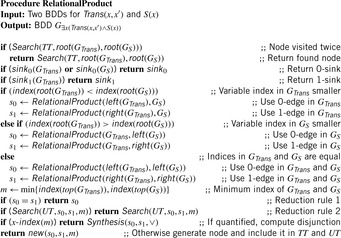
7.5 How many Boolean functions  do we have? Show that the number of (reduced-ordered) BDD representations is exactly the same.
7.6 Supply pseudo-code implementations for the main BDD operations.
1. Substitution by constant with integrated reduction rule application.
2. SAT-count backing up countervalues at internal nodes.
7.7 Give a 64-bit binary encoding for the Fifteen-Puzzle.
1. Depict the characteristic function for the goal state in this encoding.
2. Explain how to compute the Manhattan distance function as a BDD in this encoding. You may start with sub-BDDs for each tile and combine the results using a relational product on temporary variables to connect them to build the overall sum.
7.8 Provide two different encoding schemes for the level-1 Sokoban instance (see Ch. 1):
1. One that encodes each ball in binary based on the index of the maze layout.
2. One that encodes each ball using one bit.
3. Try to improve your encoding, for example, by omitting squares that can be excluded in finding a solution.
4. How many variables do you need?
5. Which one is the better encoding and how would you encode the man?
7.9 Provide an encoding for states and actions for Strips-type planning problems (see Ch. 1). Show how to combine the operator encodings to a monolithic transition relation. You may use one bit for each grounded proposition to obtain a state descriptor with  bits. Take care of propositions that are not mentioned in the initial or goal state.
7.10 Display the transition relation Trans for the Sliding-Token Puzzle for an interleaved ordering.
7.11 Perform a partitioned BFS exploration based on the set of transitions  ,
,  , and
, and  that modify variable
  , as well as
  and
and  that modify variable
  . The starting node is
  .
.
7.12 Give a consistent and nonredundant rule set for the academic knowledge database verification example.
1. Display the BDDs for all instantiated rules.
2. Compute the BDD labels that are reached in a forward chaining algorithm.
7.13 Draw the BDD for representing exactly b balls in room B in the Gripper domain.
7.14 Prove that the expressions that are generated in a labeling approach in a knowledge-based system can require exponential size, with the exponent being in the depth of the rule set.
7.15 For admissible heuristics there might be successors that address a bucket below the fmin diagonal in A*. Moreover, for explicit search we have seen that always considering the smallest bucket as in A* may lead to an exponential number of reopenings.
Show that for admissible estimates there exists an implementation of A* for which the number of images can be bounded by  .
.
7.16 The bucket-based implementation of Dijkstra's algorithm is as follows. In one iteration we first choose the bucket with the minimum f-value together with the BDD Min of all states in the priority queue having this value. Next, the partitioned transition relation  with
with  is applied to determine the BDD for the subset of all successor states that can be reached with cost i. To attach new f-values to this set, we simply insert the result into bucket
  . The pseudo code is shown in Algorithm 7.12.
1. Give a slightly more compact implementation for the priority queue using a 1-Level Bucket priority queue (see Ch. 3).
Integrate duplicate elimination to the algorithm.
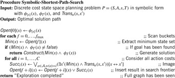
7.17 In the extension of symbolic A* to discrete weights shown in Algorithm 7.13, we determine all successors of the set of states with the minimum f-value, current cost total g, and action cost i. It remains to determine their h-values by a lookup in a (multiple)-pattern database.
1. Annotate the pseudo code with comments.
2. Perform the lookup and the combination of multiple-pattern databases  entries on-the-fly (either by taking the sum or the max). Provide pseudo code.
3. Prove that for transition weights  , and the algorithm finds the optimal solution with at most
  images, where
  is the optimal solution cost.

7.18 Adapt the symbolic branch-and-bound algorithm to a cost-optimal search with a monotonic-increasing objective function  represented as a BDD.
7.19 BDDs can serve alternative data structures for solving the Subset Query or Containment Query problem (see Ch. 3). The characteristic function of each encountered pattern is taken into disjunct with the Boolean representation of the subset dictionary. In the example of Sokoban, if variable  denotes the existence of a ball at position i, we build the following Boolean function:
1. Denote how to add a pattern into the pattern store and derive its time complexity for insertion.
2. Denote how to search a position for a contained pattern in the pattern store and derive the time complexity of the operation.
7.11. Bibliographic Notes
BDDs together with efficient operations on them have been made prominent by Bryant (1992), but binary decision diagrams go back to Lee (1959) and Akers (1978). Minato, Ishiura, and Yajima (1990) have shown how to store several BDDs in a joint structure. One of the best libraries is CUDD, maintained by Fabio Somenzi. Improved implementation issues are found in Yang et al. (1998). The authors have shown that the number of subproblem disjunctions is a good platform-independent measure of the work to be performed in computing the image. Lower bounds and some generalized BDD structures have been studied by Sieling (1994). A survey on theory and applications of BDDs has been given by Wegener (2000).
The use of BDDs for model checking, known as symbolic model checking, has been introduced by McMillan (1993). Implementations for symbolic model checkers based on BDDs include nuSMV by Cimatti, Giunchiglia, Giunchiglia, and Traverso (1997) and μcke by Biere (1997). Alternatives for symbolic exploration with BDDs are bounded model checkers introduced by Biere, Cimatti, Clarke, and Zhu (1999) that base on thresholded Sat solving as in the Satplan system by Kautz and Selman (1996). The rise of heuristic search procedures for explicit and symbolic model checking tools (e.g., by Edelkamp, Leue, and Lluch-Lafuente, 2004b and by Qian and Nymeyer, 2004) indicate that synergies between the disciplines are many-fold.
Symbolic A* (alias BDDA*) has been invented by Edelkamp and Reffel (1998) in the context of solving the (n2−1)-Puzzle and Sokoban. The work estimated the maximum number of iterations. The algorithm has been ported to hardware verification problems (Reffel and Edelkamp, 1999) and has been integrated in the presented planning context by Edelkamp and Helmert (2001). ADDA* developed by Hansen, Zhou, and Feng (2002) is an alternative implementation of symbolic A* with ADDs. Jensen, Bryant, and Veloso (2002) have refined the partitioning in symbolic A*. The authors also have exploited on a matrix representation of g-values and h-values. An extensive treatment, including applications in nondeterministic and adversarial domains, has been provided by Jensen (2003). Symbolic branch-and-bound search has been proposed by Jensen, Hansen, Richards, and Zhou (2006).
In an experimental study, Qian and Nymeyer (2003) indicated that for BDD exploration with heuristics with smaller range and inducing a simpler BDD structure, sometimes to speedup the overall search process better than more complex heuristics (having more involved BDDs). However, this has not been shown to be a general trend.
Different symbolic approaches are under theoretical and empirical investigation for classic graph algorithms. The used upper bound O(2n/n) for the BDD size on n variables is due to the work of Breitbart, Hunt, and Rosenkrantz (1995). In fact, Breitbart, Hunt, and Rosenkrantz (1992) already have determined this lower bound and a matching upper bound function. The presented study for Topological Sorting has been proposed by Woelfel (2006). Maximum Flow has been studied by Hachtel and Somenzi (1992), with an improvement given by Sawatzki (2004b). A treatment for shortest paths based on a symbolical representation of the entire state space is also subject to current research; for example, the All-Pairs Shortest Path problem has been considered by Sawatzki (2004a).
..................Content has been hidden....................
You can't read the all page of ebook, please click here login for view all page.