
Chapter 11. Real-Time Search
Sven Koenig
The on-line search algorithms in this chapter interleave searches and action executions. They decide on a local search space, search it, and determine which actions to execute within it. Then, they execute these actions and repeat the process from their new state until they reach a goal state.
Keywords: agent-centered search, convergence detection and speed-up, coverage, edge counting, fast h-value updates, fast learning and converging search (FALCONS), goal-directed navigation (in known and unknown terrain), learning real-time A* (LRTA*), localization, local search space, minimal lookahead, min-max learning real-time A* (min-max LRTA*), node counting, non-deterministic state space, on-line search, probabilistic learning real-time A* (probabilistic LRTA*), probabilistic state space, real-time A* (RTA*), real-time adaptive A* (RTAA*), real-time (heuristic) search, robot navigation, safely-explorable state space
A real-time search method that does not satisfy our definition but only needs a constant search time before the first action execution and between action executions, for example, has been described by Parberry (1995). Moreover, there is a line of work done by Carlos Hernndez and Pedro Meseguer on real-time search with significant improvements to LRTA* (Hernández and Meseguer, 2005, 2007a,b).
In this chapter, we describe real-time (heuristic) search and illustrate it with examples. Real-time search is sometimes used to describe search methods that only need a constant search time between action executions. However, we use a more restrictive definition of real-time search in this chapter, namely that of real-time search as a variant of agent-centered search. Interleaving or overlapping searches and action executions often has advantages for intelligent systems (agents) that interact directly with the world. Agent-centered search restricts the search to the part of the state space around the current state of the agent; for example, the current position of a mobile robot or the current board position of a game. The part of the state space around the current state of the agent is the part of the state space that is immediately relevant for the agent in its current situation (because it contains the states that the agent will soon be in) and sometimes might be the only part of the state space that the agent knows about. Agent-centered search usually does not search all the way from the start state to a goal state. Instead, it decides on the local search space, searches it, and determines which actions to execute within it. Then, it executes these actions (or only the first action) and repeats the process from its new state until it reaches a goal state.
The best-known example of agent-centered search is probably game playing, such as playing Chess (as studied in Chapter 12). In this case, the states correspond to board positions and the current state corresponds to the current board position. Game-playing programs typically perform a minimax search with a limited lookahead (i.e., search horizon) around the current board position to determine which move to perform next. The reason for performing only a limited local search is that the state spaces of realistic games are too large to perform complete searches in a reasonable amount of time and with a reasonable amount of memory. The future moves of the opponent cannot be predicted with certainty, which makes the search tasks nondeterministic. This results in an information limitation that can only be overcome by enumerating all possible moves of the opponent, which results in large search spaces. Performing agent-centered search allows game-playing programs to choose a move in a reasonable amount of time while focusing on the part of the state space that is the most relevant to the next move decision.
Traditional search methods, such as A*, first determine minimal-cost paths and then follow them. Thus, they are offline search methods. Agent-centered search methods, on the other hand, interleave search and action execution and are thus online search methods. They can be characterized as revolving search methods with greedy action-selection steps that solve suboptimal search tasks. They are suboptimal since they are looking for any path (i.e., sequence of actions) from the start state to a goal state. The sequence of actions that agent-centered search methods execute is such a path. They are revolving, because they repeat the same process until they reach a goal state. Agent-centered search methods have the following two advantages:
Time constraints: Agent-centered search methods can execute actions in the presence of soft or hard time constraints since the sizes of their local search spaces are independent of the sizes of the state spaces and can thus remain small. The objective of the search in this case is to approximately minimize the execution cost subject to the constraint that the search cost (here: runtime) between action executions is bounded from above, for example, in situations where it is more important to act reasonably in a timely manner than to minimize the execution cost after a long delay. Examples include steering decisions when driving a car or movement decisions when crossing a busy street.
Sum of search and execution cost: Agent-centered search methods execute actions before their complete consequences are known and thus are likely to incur some overhead in terms of the execution cost, but this is often outweighed by a decrease in the search cost, both because they trade off the search and execution cost and because they allow agents to gather information early in nondeterministic state spaces, which reduces the amount of search they have to perform for unencountered situations. Thus, they often decrease the sum of the search and execution cost compared to search methods that first determine minimal-cost paths and then follow them, which can be important for search tasks that need to be solved only once.
Agent-centered search methods have to ensure that they do not cycle without making progress toward a goal state. This is a potential problem since they execute actions before their consequences are completely known. Agent-centered search methods have to ensure both that it remains possible to achieve the goal and that they eventually do so. The goal remains achievable if no actions exist of which the execution makes it impossible to reach a goal state, if the agent-centered search methods can avoid the execution of such actions in case they do exist, or if the agent-centered search methods have the ability to reset the agent into the start state. Real-time search methods are agent-centered search methods that store a value, called h-value, in memory for each state that they encounter during the search and update them as the search progresses, both to focus the search and avoid cycling, which accounts for a large chunk of their search time per search episode.
11.1. LRTA*
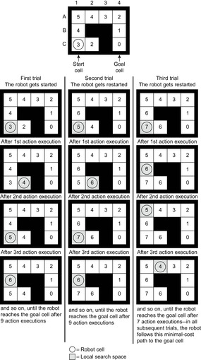
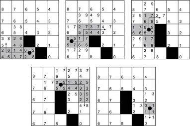
Learning real-time A* (LRTA*) is probably the most popular real-time search method, and we relate all real-time search methods in this chapter to it. The h-values of LRTA* approximate the goal distances of the states. They can be initialized using a heuristic function. They can be all zero if more informed h-values are not available. Figure 11.1 illustrates the behavior of LRTA* using a simplified goal-directed navigation task in known terrain without uncertainty about the start cell. The robot can move one cell to the north, east, south, or west (unless that cell is blocked). All action costs are one. The task of the robot is to navigate to the given goal cell and then stop. In this case, the states correspond to cells, and the current state corresponds to the current cell of the robot. We assume that there is no uncertainty in actuation and sensing. The h-values are initialized with the Manhattan distances. A robot under time pressure could reason as follows: Its current cell C1 is not a goal cell. Thus, it needs to move to one of the cells adjacent to its current cell to get to a goal cell. The cost-to-go of an action is its action cost plus the estimated goal distance of the successor state reached when executing the action, as given by the h-value of the successor state. If it moves to cell B1, then the action cost is one and the estimated goal distance from there is four as given by the h-value of cell B1. The cost-to-go of moving to cell B1 is thus five. Similarly, the cost-to-go of moving to cell C2 is three. Thus, it looks more promising to move to cell C2. Figure 11.2 visualizes the h-value surface formed by the initial h-values. However, a robot does not reach the goal cell if it always executes the move with the minimal cost-to-go and thus performs steepest descent on the initial h-value surface. It moves back and forth between cells C1 and C2 and thus cycles forever due to the local minimum of the h-value surface at cell C2.
 |
| Figure 11.1 |
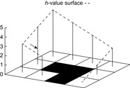 |
| Figure 11.2 Initial h-value surface, by Koenig (2001). |
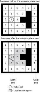
We could avoid this problem by randomizing the action-selection process slightly, possibly together with resetting the robot into a start state (random restart) after the execution cost has become large. LRTA*, however, avoids this problem by increasing the h-values to fill the local minima in the h-value surface. Figure 11.3 shows how LRTA* performs a search around the current state of the robot to determine which action to execute next if it breaks ties among actions in the following order: north, east, south, and west. It operates as follows:
Local Search Space–Generation Step: LRTA* decides on the local search space. The local search space can be any set of nongoal states that contains the current state. We say that a local search space is minimal if and only if it contains only the current state. We say that it is maximal if and only if it contains all nongoal states. In Figure 11.1, for example, the local search spaces are minimal. In this case, LRTA* can construct a search tree around the current state. The local search space consists of all nonleaves of the search tree. Figure 11.3 shows the search tree for deciding which action to execute in the start cell C1.
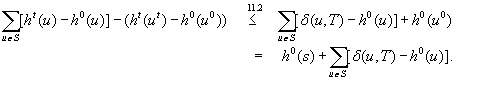
Value-Update Step: LRTA* assigns each state in the local search space its correct goal distance under the assumption that the h-values of the states just outside of the local search space correspond to their correct goal distances. In other words, it assigns each state in the local search space the minimum of the execution cost for getting from it to a state just outside of the local search space, plus the estimated remaining execution cost for getting from there to a goal state, as given by the h-value of the state just outside of the local search space. The reason for this is that the local search space does not include any goal state. Thus, a minimal-cost path from a state in the local search space to a goal state has to contain a state just outside of the local search space. Thus, the smallest estimated cost of all paths from the state via a state just outside of the local search space to a goal state is an estimate of the goal distance of the state. Since this lookahead value is a more accurate estimate of the goal distance of the state in the local search space, LRTA* stores it in memory, overwriting the existing h-value of the state.
In the example, the local search space is minimal and LRTA* can simply update the h-value of the state in the local search space according to the following rule provided that it ignores all actions that can leave the current state unchanged. LRTA* first assigns each leaf of the search tree the h-value of the corresponding state. The leaf that represents cell B1 is assigned an h-value of four, and the leaf that represents cell C2 is assigned an h-value of two. This step is marked in Figure 11.3. The new h-value of the root of the search tree, that represents cell C1, then is the minimum of the costs-to-go of the actions that can be executed in it, that is, the minimum of five and three. ②. This h-value is then stored in memory for cell C1 . Figure 11.4 shows the result of one value-update step for a different example where the local search space is nonminimal.
Action-Selection Step: LRTA* selects an action for execution that is the beginning of a path that promises to minimize the execution cost from the current state to a goal state (ties can be broken arbitrarily). In the example, LRTA* selects the action with the minimal cost-to-go. Since moving to cell B1 has cost-to-go five and moving to cell C2 has cost-to-go three, LRTA* decides to move to cell C2.
Action-Execution Step: LRTA* executes the selected action and updates the state of the robot, and repeats the process from the new state of the robot until the robot reaches a goal state. If its new state is outside of the local search space, then it needs to repeat the local search space–generation and value-update steps. Otherwise, it can repeat these steps or proceed directly to the action-selection step. Executing more actions before generating the next local search space typically results in a smaller search cost (because LRTA* needs to search less frequently); executing fewer actions typically results in a smaller execution cost (because LRTA* selects actions based on more information).
 |
| Figure 11.3 Illustration of LRTA*, by Koenig (2001). |
 |
| Figure 11.4 LRTA* with a larger local search space, by Koenig (2001). |
The left column of Figure 11.1 shows the result of the first couple of steps of LRTA* for the example. The values in grey cells are the new h-values calculated by the value-update step because the corresponding cells are part of the local search space. The robot reaches the goal cell after nine action executions; that is, with execution cost nine. We assumed here that the terrain is known and the reason for using real-time search is time pressure. Another reason for using real-time search could be missing knowledge of the terrain and the resulting desire to restrict the local search spaces to the known parts of the terrain.
We now formalize LRTA*, using the following assumptions and notation for deterministic and nondeterministic search tasks, which will be used throughout this chapter: S denotes the finite set of states of the state space,  the start state, and
  the set of goal states.
  denotes the finite, nonempty set of (potentially nondeterministic) actions that can be executed in state
  .
.  denotes the action cost that results from the execution of action
  in state
  . We assume that all action costs are one unless stated otherwise.
 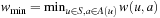 denotes the minimal action cost of any action.
  denotes the set of successor states that can result from the execution of action
  in state
  .
.  denotes the state that results from an actual execution of action
  in state
  . In deterministic state spaces,
  contains only one state, and we use
  also to denote this state. Thus,
 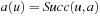 in this case. An agent starts in the start state and has to move to a goal state. The agent always observes what its current state is and then has to select and execute its next action, which results in a state transition to one of the possible successor states. The search task is solved when the agent reaches a goal state. We denote the number of states by
  and the number of state-action pairs (loosely called actions) by
  ; that is, an action that is applicable in more than one state counts more than once. Moreover, δ (u, T) ≥ 0 denotes the goal distance of state
  ; that is, the minimal execution cost with which a goal state can be reached from state u. The depth d of the state space is its maximal goal distance,
 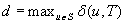 . The expression
  returns one of the elements
  that minimize f (x); that is, one of the elements from the set
  . We assume that all search tasks are deterministic unless stated otherwise, and discuss nondeterministic state spaces in 11.5.7 and 11.6.4.

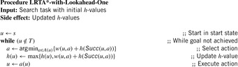
Algorithm 11.1 shows pseudo code for LRTA* in deterministic state spaces. It associates a nonnegative h-value h (u) with each state  . In practice, they are not initialized upfront but rather can be initialized as needed. LRTA* consists of a termination-checking step, a local search space–generation step, a value-update step, an action-selection step, and an action-execution step. LRTA* first checks whether it has already reached a goal state and thus can terminate successfully. If not, it generates the local search space
  . Although we require only that
  and
and  , in practice LRTA* often uses forward search (that searches from the current state to the goal states) to select a continuous part of the state space around the current state u of the agent. LRTA* could determine the local search space, for example, with a breadth-first search around state u up to a given depth or with a (forward) A* search around state u until a given number of states have been expanded (or, in both cases, a goal state is about to be expanded). The states in the local search space correspond to the nonleaves of the corresponding search tree, and thus are all nongoal states. In Figure 11.1, a (forward) A* search that expands two states picks a local search space that consists of the expanded states C1 and C2. LRTA* then updates the h-values of all states in the local search space. Based on these h-values, LRTA* decides which action to execute next. Finally, it executes the selected action, updates its current state, and repeats the process.
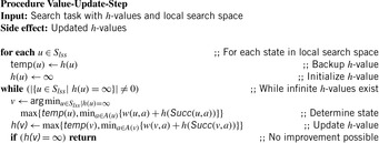
Algorithm 11.2 shows how LRTA* updates the h-values in the local search space using a variant of Dijkstra's algorithm. It assigns each state its goal distance under the assumption that the h-values of all states in the local search space do not overestimate the correct goal distances and the h-values of all states outside of the local search space correspond to their correct goal distances. It does this by first assigning infinity to the h-values of all states in the local search space. It then determines a state in the local search space of which the h-value is still infinity and which minimizes the maximum of its previous h-value and the minimum over all actions in the state of the cost-to-go of the action. This value then becomes the h-value of this state, and the process repeats. The way the h-values are updated ensures that the states in the local search space are updated in the order of their increasing new h-values. This ensures that the h-value of each state in the local search space is updated at most once. The method terminates when either the h-value of each state in the local search space has been assigned a finite value or an h-value would be assigned the value infinity. In the latter case, the h-values of all remaining states in the local search space would be assigned the value infinity as well, which is already their current value.
Lemma 11.1
For all times t = 0, 1, 2,… (until termination): Consider the (t + 1) st value-update step of LRTA* (i.e., call to procedure Value-Update-Step inAlgorithm 11.1). Let  refer to its local search space. Let
  and
and  refer to the h-values immediately before and after, respectively, the value-update step. Then, for all states
  , the value-update step terminates with
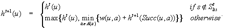
Proof
by induction on the number of iterations within the value-update step (see Exercises).
Lemma 11.2
Admissible initial h-values (that is, initial h-values that are lower bounds on the corresponding goal distances) remain admissible after every value-update step of LRTA* and are monotonically nondecreasing. Similarly, consistent initial h-values (i.e., initial h-values that satisfy the triangle inequality) remain consistent after every value-update step of LRTA* and are monotonically nondecreasing.
Proof
by induction on the number of value-update steps, using Lemma 11.1 (see Exercises).
After the value-update step has updated the h-values, LRTA* greedily chooses the action  in the current nongoal state u with the minimal cost-to-go
  for execution to minimize the estimated execution cost to a goal state. Ties can be broken arbitrarily, although we explain later that tie breaking can be important. Then, LRTA* has a choice. It can generate another local search space, update the h-values of all states that it contains, and select another action for execution. This version of LRTA* results when the repeat-until loop in Algorithm 11.1 is executed only once, which is why we refer to this version as LRTA* without repeat-until loop. If the new state is still part of the local search space (the one that was used to determine the action of which the execution resulted in the new state), LRTA* can also select another action for execution based on the current h-values. This version of LRTA* results when the repeat-until loop in Algorithm 11.1 is executed until the new state is no longer part of the local search space (as shown in the pseudo code), which is why we refer to this version as LRTA* with repeat-until loop. It searches less often and thus tends to have smaller search costs but larger execution costs. We analyze LRTA* without repeat-until loop, which is possible because LRTA* with repeat-until loop is a special case of LRTA* without repeat-until loop. After LRTA* has used the value-update step on some local search space, the h-values do not change if LRTA* uses the value-update step again on the same local search space or a subset thereof. Whenever LRTA* repeats the body of the repeat-until loop, the new current state is still part of the local search space Slss and thus not a goal state. Consequently, LRTA* could now search a subset of Slss that includes the new current state, for example, using a minimal local search space, which does not change the h-values and thus can be skipped.
11.2. LRTA* with Lookahead One
We now state a variant of LRTA* with minimal local search spaces, the way it is often stated in the literature. Algorithm 11.3 shows the pseudo code of LRTA* with lookahead one. Its action-selection step and value-update step can be explained as follows. The action-selection step greedily chooses the action  in the current nongoal state u with the minimal cost-to-go
  for execution to minimize the estimated execution cost to a goal state. (The cost-to-go
  is basically the f-value of state
  of an A* search from u toward the goal states.) The value-update step replaces the h-value of the current state with a more accurate estimate of the goal distance of the state based on the costs-to-go of the actions that can be executed in it, which is similar to temporal difference learning in reinforcement learning. If all h-values are admissible, then both h (u) and the minimum of the costs-to-go of the actions that can be executed in state u are lower bounds on its goal distance, and the larger of these two values is the more accurate estimate. The value-update step then replaces the h-value of state u with this value. The value-update step of LRTA* is sometimes stated as
  . Our slightly more complex variant guarantees that the h-values are nondecreasing. Since the h-values remain admissible and larger admissible h-values tend to guide the search better than smaller admissible h-values, there is no reason to decrease them. If the h-values are consistent then both value-update steps are equivalent. Thus, LRTA* approximates Bellman's optimal condition for minimal-cost paths in a way similar to Dijkstra's algorithm. However, the h-values of LRTA* with admissible initial h-values approach the goal distances from below and are monotonically nondecreasing, while the corresponding values of Dijkstra's algorithm approach the goal distances from above and are monotonically nonincreasing.
LRTA* with lookahead one and LRTA* with minimal local search spaces behave identically in state spaces where the execution of all actions in nongoal states necessarily results in a state change, that is, it cannot leave the current state unchanged. In general, actions that are not guaranteed to result in a state change can safely be deleted from state spaces because there always exists a path that does not include them (such as the minimal-cost path), if there exists a path at all. LRTA* with arbitrary local search spaces, including minimal and maximal local search spaces, never executes actions whose execution can leave the current state unchanged but LRTA* with lookahead one can execute them. To make them identical, one can change the action-selection step of LRTA* with lookahead one to “ . However, this is seldom done in the literature.
In the following, we refer to LRTA* as shown in Algorithm 11.1 and not to LRTA* with lookahead one as shown in Algorithm 11.3 when we analyze the execution cost of LRTA*.
11.3. Analysis of the Execution Cost of LRTA*
A disadvantage of LRTA* is that it cannot solve all search tasks. This is so because it interleaves searches and action executions. All search methods can solve only search tasks for which the goal distance of the start state is finite. Interleaving searches and action executions limits the solvable search tasks because actions are executed before their complete consequences are known. Thus, even if the goal distance of the start state is finite, it is possible that LRTA* accidentally executes actions that lead to a state with infinite goal distance, such as actions that “blow up the world," at which point the search task becomes unsolvable for the agent. However, LRTA* is guaranteed to solve all search tasks in safely explorable state spaces. State spaces are safely explorable if and only if the goal distances of all states are finite; that is, the depth is finite. (For safely explorable state spaces where all action costs are one, it holds that  .) To be precise: First, all states of the state space that cannot possibly be reached from the start state, or can be reached from the start state only by passing through a goal state, can be deleted. The goal distances of all remaining states have to be finite. Safely explorable state spaces guarantee that LRTA* is able to reach a goal state no matter which actions it has executed in the past. Strongly connected state spaces (where every state can be reached from every other state), for example, are safely explorable. In state spaces that are not safely explorable, LRTA* either stops in a goal state or reaches a state with goal distance infinity and then executes actions forever. We could modify LRTA* to use information from its local search spaces to detect that it can no longer reach a goal state (e.g., because the h-values have increased substantially) but this is complicated and seldom done in the literature. In the following, we assume that the state spaces are safely explorable.
LRTA* always reaches a goal state with a finite execution cost in all safely explorable state spaces, as can be shown by contradiction (the cycle argument ). If LRTA* did not reach a goal state eventually, then it would cycle forever. Since the state space is safely explorable, there must be some way out of the cycle. We show that LRTA* eventually executes an action that takes it out of the cycle, which is a contradiction: If LRTA* did not reach a goal state eventually, it would execute actions forever. In this case, there is a time t after which LRTA* visits only those states again that it visits infinitely often; it cycles in part of the state space. The h-values of the states in the cycle increase beyond any bound, since LRTA* repeatedly increases the h-value of the state with the minimal h-value in the cycle by at least the minimal action cost wmin of any action. It gets into a state u with the minimal h-value in the cycle and all of its successor states then have h-values that are no smaller than its own h-value. Let h denote the h-values before the value-update step and h′ denote the h-values after the value-update step. According to Lemma 11.1, the h-value of state u is then set to 

 . In particular, the h-values of the states in the cycle rise by arbitrarily large amounts above the h-values of all states that border the cycle. Such states exist since a goal state can be reached from every state in safely explorable state spaces. Then, however, LRTA* is forced to visit such a state after time t and leave the cycle, which is a contradiction.
The performance of LRTA* is measured by its execution cost until it reaches a goal state. The complexity of LRTA* is its worst-case execution cost over all possible topologies of state spaces of the same sizes, all possible start and goal states, and all tie-breaking rules among indistinguishable actions. We are interested in determining how the complexity scales as the state spaces get larger. We measure the sizes of state spaces as nonnegative integers and use measures x, such as x = nd, the product of the number of states and the depth. An upper complexity bound Ox has to hold for every x that is larger than some constant. Since we are mostly interested in the general trend (but not outliers) for the lower complexity bound, a lower complexity bound Ω (x) has to hold only for infinitely many different x. Furthermore, we vary only x. If x is a product, we do not vary both of its factors independently. This is sufficient for our purposes. A tight complexity bound  means both Oxand
  . To be able to express the complexity in terms of the number of states only, we often make the assumption that the state spaces are reasonable. Reasonable state spaces are safely explorable state spaces with
  (or, more generally, state spaces of which the number of actions does not grow faster than the number of states squared). For example, safely explorable state spaces where the execution of different actions in the same state results in different successor states are reasonable. For reasonable state spaces where all action costs are one, it holds that
  and
and  . We also study Eulerian state spaces. A Eulerian state space is a state space where there are as many actions that leave a state as there are actions that enter it. For example, undirected state spaces are Eulerian. An undirected state space is a state space where every action in a state u of which the execution results in a particular successor state v has a unique corresponding action in state v of which the execution results in state u.
11.3.1. Upper Bound on the Execution Cost of LRTA*
In this section, we provide an upper bound on the complexity of LRTA* without repeat-until loop. Our analysis is centered around the invariant from Lemma 11.3. The time superscript t refers to the values of the variables immediately before the (t + 1) st value-update step of LRTA*. For instance, u0 denotes the start state s and  the action executed directly after the (t + 1) st value-update step. Similarly,
  denotes the h-values before the (t + 1) st value-update step and
  denotes the h-values after the
  st value-update step. In the following, we prove an upper bound on the execution cost after which LRTA* is guaranteed to reach a goal state in safely explorable state spaces.
Lemma 11.3
For all times t = 0,1,2,… (until termination) it holds that the execution cost of LRTA* with admissible initial h-values h0 at time t is at most  . (Sums have a higher precedence than other operators. For example,
  .)
.)
Proof
by induction: The h-values are admissible at time t according to Lemma 11.2. Thus, they are bounded from above by the goal distances, which are finite since the state space is safely explorable. For t = 0, the execution cost and its upper bound are both zero, and the lemma thus holds. Now assume that the theorem holds at time t. The execution cost increases by  and the upper bound increases by
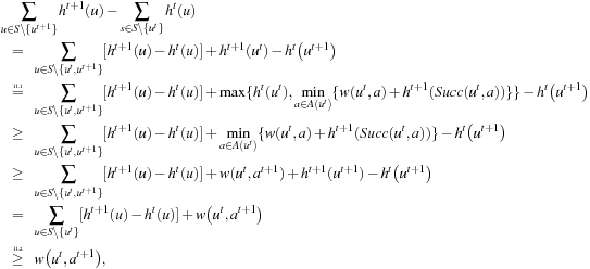 and the lemma thus continues to hold.
Theorem 11.1 uses Lemma 11.3 to derive an upper bound on the execution cost.
Theorem 11.1
(Completeness of LRTA*) LRTA* with admissible initial h-values h0 reaches a goal state with an execution cost of at most  .
.
Proof
Since the goal distances are finite in safely explorable state spaces and the minimal action cost wmin of any action is strictly positive, Theorem 11.1 shows that LRTA* with admissible initial h-values reaches a goal state after a bounded number of action executions in safely explorable state spaces; that is, it is complete. More precisely: LRTA* reaches a goal state with an execution cost of at most  , and thus after at most
  action executions. Thus, it reaches a goal state with finite execution cost in safely explorable state spaces. One consequence of this result is that search tasks in state spaces where all states are clustered around the goal states are easier to solve with LRTA* than search tasks in state spaces that do not possess this property. Consider, for example, sliding-tile puzzles, which are sometimes considered to be hard search tasks because they have a small goal density. The Eight-Puzzle has 181,440 states but only one goal state. However, the average goal distance of the Eight-Puzzle (with the goal configuration where the tiles form a ring around the center) is only 21.5 and its maximal goal distance is only 30. This implies that LRTA* never moves far away from the goal state even if it makes a mistake and executes an action that does not decrease the goal distance. This makes the Eight-Puzzle easy to search with LRTA* relative to other state spaces with the same number of states.
11.3.2. Lower Bound on the Execution Cost of LRTA*
LRTA* reaches a goal state with an execution cost of at most  , and it holds that
 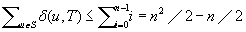 in safely explorable state spaces where all action costs are one. Now assume that LRTA* with minimal local search spaces is zero-initialized, which implies that it is uninformed. In the following, we show that the upper complexity bound is then tight for infinitely many n. Figure 11.5 shows an example for which the execution cost of zero-initialized LRTA* with minimal local search spaces is
  in the worst case until it reaches a goal state. The upper part of the figure shows the state space. All action costs are one. The states are annotated with their goal distances, their initial h-values, and their names. The lower part of the figure shows the behavior of LRTA*. On the right, the figure shows the state space with the h-values after the value-update step but before the action-execution step. The current state is shown in bold. On the left, the figure shows the searches that resulted in the h-values shown on the right. Again, the states are annotated with their h-values after the value-update step but before the action-execution step. The current state is on top. Ellipses show the local search spaces, and dashed lines show the actions that LRTA* is about to execute. For the example search task, after LRTA* has visited a state for the first time, it has to move through all previously visited states again before it is able to visit another state for the first time. Thus, the execution cost is quadratic in the number of states. If LRTA* breaks ties in favor of successor states with smaller indices, then its execution cost f (n) until it reaches the goal state satisfies the recursive equations
  and
and  . Thus, its execution cost is
  (for
(for  ). The execution cost equals exactly the sum of the goal distances because LRTA* was zero-initialized and its final h-values are equal to the goal distances. For example,
  for n = 5. In this case, LRTA* follows the path s1, s2, s1, s3, s2, s1, s4, s3, s2, s1, and s5.
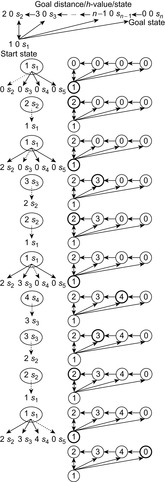 |
| Figure 11.5 LRTA* in a state space with worst-case execution cost, by Koenig (2001). |
Overall, the previous section showed that the complexity of zero-initialized LRTA* with minimal local search spaces is  over all state spaces where all actions costs are one, and the example in this section shows that it is
  . Thus, the complexity is
  over all state spaces where all actions costs are one and
  over all safely explorable state spaces where all actions costs are one (see Exercises).
11.4. Features of LRTA*
In this section, we explain the three key features of LRTA*.
11.4.1. Heuristic Knowledge
LRTA* uses heuristic knowledge to guide its search. The larger its initial h-values, the smaller the upper bound on its execution cost provided by Theorem 11.1. For example, LRTA* is fully informed if and only if its initial h-values equal the goal distances of the states. In this case, Theorem 11.1 predicts that the execution cost is at most  until LRTA* reaches a goal state. Thus, its execution cost is worst-case optimal and no other search method can do better in the worst case. In general, the execution cost is the smaller the more informed the initial h-values are although this correlation is not guaranteed to be perfect.
11.4.2. Fine-Grained Control
LRTA* allows for fine-grained control over how much search to perform between action executions by varying the sizes of its local search spaces. For example, LRTA* with repeat-until loop and maximal or, more generally, sufficiently large local search spaces performs a complete search without interleaving searches and action executions, which is slow but produces minimal-cost paths and thus minimizes the execution cost. On the other hand, LRTA* with minimal local search spaces performs almost no searches between action executions. There are several advantages to this fine-grained control.
In the presence of time constraints, LRTA* can be used as an anytime contract algorithm for determining which action to execute next, which allows it to adjust the amount of search performed between action executions to the search and execution speeds of robots or the time a player is willing to wait for a game-playing program to make a move. Anytime contract algorithms are search methods that can solve search tasks for any given bound on their search cost, so that their solution quality tends to increase with the available search cost.
The amount of search between action executions does not only influence the search cost but also the execution cost and thus also the sum of the search and execution cost. Typically, reducing the amount of search between action executions reduces the (overall) search cost but increases the execution cost (because LRTA* selects actions based on less information), although theoretically the search cost could also increase if the execution cost increases sufficiently (because LRTA* performs more searches). The amount of search between action executions that minimizes the sum of the search and execution cost depends on the search and execution speeds of the agent.
Fast-acting agents: A smaller amount of search between action executions tends to benefit agents of which the execution speed is sufficiently fast compared to their search speed since the resulting increase in execution cost is small compared to the resulting decrease in search cost, especially if heuristic knowledge focuses the search sufficiently well. For example, the sum of the search and execution cost approaches the search cost as the execution speed increases, and the search cost can often be reduced by reducing the amount of search between action executions. When LRTA* is used to solve search tasks offline, it only moves a marker within the computer (that represents the state of a fictitious agent), and thus action execution is fast. Small local search spaces are therefore optimal for solving sliding-tile puzzles with the Manhattan distance.
Slow-acting agents: A larger amount of search between action executions is needed for agents of which the search speed is sufficiently fast compared to their execution speed. For example, the sum of the search and execution cost approaches the execution cost as the search speed increases, and the execution cost can often be reduced by increasing the amount of search between action executions. Most robots are examples of slow-acting agents.
We will discuss later in this chapter that larger local search spaces sometimes allow agents to avoid executing actions from which they cannot recover in state spaces that are not safely explorable. On the other hand, larger local search spaces might not be practical in state spaces that are not known in advance and need to get learned during execution since there can be an advantage to restricting the search to the known part of the state space.
11.4.3. Improvement of Execution Cost
If the initial h-values are not completely informed and the local search spaces are small, then it is unlikely that the execution cost of LRTA* is minimal. In Figure 11.1, for example, the robot could reach the goal cell in seven action executions. However, LRTA* improves its execution cost, although not necessarily monotonically, as it solves search tasks with the same set of goal states (even with different start states) in the same state spaces until its execution cost is minimal; that is, until it has converged. Thus, LRTA* can always have a small sum of search and execution cost and still minimize the execution cost in the long run in case similar search tasks unexpectedly repeat, which is the reason for the “learning” in its name. Assume that LRTA* solves a series of search tasks in the same state space with the same set of goal states. The start states need not be identical. If the initial h-values of LRTA* are admissible for the first search task, then they are also admissible for the first search task after LRTA* has solved the search task and are statewise at least as informed as initially. Thus, they are also admissible for the second search task and LRTA* can continue to use the same h-values across search tasks. The start states of the search tasks can differ since the admissibility of h-values does not depend on them. This way, LRTA* can transfer acquired knowledge from one search task to the next one, thereby making its h-values more informed. Ultimately, more informed h-values result in an improved execution cost, although the improvement is not necessarily monotonic. (This also explains why LRTA* can be interrupted at any state and resume execution at a different state.) The following theorems formalize this knowledge transfer in the mistake-bounded error model. The mistake-bounded error model is one way of analyzing learning methods by bounding the number of mistakes that they make. Here, it counts as one mistake when LRTA* reaches a goal state with an execution cost that is larger than the goal distance of the start state and thus does not follow a minimal-cost path from the start state to a goal state.
Theorem 11.2
(Convergence of LRTA*) Assume that LRTA* maintains h-values across a series of search tasks in the same safely explorable state space with the same set of goal states. Then, the number of search tasks for which LRTA* with admissible initial h-values reaches a goal state with an execution cost of more than δ (s, T) (where s is the start state of the current search task) is bounded from above.
Proof
It is easy to see that the agent follows a minimal-cost path from the start state to a goal state if it follows a path from the start state to a goal state where the h-value of every state is equal to its goal distance. If the agent does not follow such a path, then it transitions at least once from a state u of which the h-value is not equal to its goal distance to a state v of which the h-value is equal to its goal distance, since it reaches a goal state and the h-value of the goal state is zero since the h-values remain admissible according to Lemma 11.2. Let a denote the action of which the execution in state u results in state v. Let h denote the h-values before the value-update step and h′ denote the h-values after the value-update step. According to Lemma 11.1, the h-value of state u is set to 

 . Thus,
  since the h-values cannot become inadmissible according to Lemma 11.2. After the h-value of state u is set to its goal distance, the h-value can no longer change since it could only increase according to Lemma 11.2 but would then make the h-values inadmissible, which is impossible according to the same lemma. Since the number of states is finite, it can happen only a bounded number of times that the h-value of a state is set to its goal distance. Thus, the number of times that the agent does not follow a minimal-cost path from the start state to a goal state is bounded.
Assume that LRTA* solves the same search task repeatedly from the same start state, and that the action-selection step always breaks ties among the actions in the current state according to a fixed ordering of the actions. Then, the h-values no longer change after a finite number of searches, and LRTA* follows the same minimal-cost path from the start state to a goal state during all future searches. (If LRTA* breaks ties randomly, then it eventually discovers all minimal-cost paths from the start state to the goal states.) Figure 11.1 (all columns) illustrates this aspect of LRTA*. In the example, LRTA* with minimal local search spaces breaks ties among successor cells in the following order: north, east, south, and west. Eventually, the robot always follows a minimal-cost path to the goal cell. Figure 11.6 visualizes the h-value surface formed by the final h-values. The robot now reaches the goal cell on a minimal-cost path if it always moves to the successor cell with the minimal h-value (and breaks ties in the given order) and thus performs steepest descent on the final h-value surface.
 |
| Figure 11.6 h-value surface after convergence, by Koenig (2001). |
11.5. Variants of LRTA*
We now discuss several variants of LRTA*.
11.5.1. Variants with Local Search Spaces of Varying Sizes
LRTA* with small local search spaces executes a large number of actions to escape from depressions (that is, valleys) in the h-value surface (see Exercises). It can avoid this by varying the sizes of its local search spaces during a search, namely by increasing the sizes of its local search spaces in depressions. For example, LRTA* can use minimal local search spaces until it reaches the bottom of a depression. It can detect this situation because then the h-value of its current state is smaller than the costs-to-go of all actions that can be executed in it (before it executes the value-update step). In this case, it determines the local search space that contains all states that are part of the depression by starting with its current state and then repeatedly adding successor states of states in the local search space to the local search space so that, once a successor state is added, the h-value of each state in the local search space is less than the cost-to-go of all actions that can be executed in it and result in successor states outside of the local search space. The local search space is complete when no more states can be added. In Figure 11.1 (left), for example, LRTA* picks the minimal local search space that contains only state C1 when it is in state C1. It notices that it has reached the bottom of a depression and picks a local search space that consists of the states B1, C1, and C2 when it is in state C2. Its value-update step then sets the h-values of B1, C1, and C2 to 6, 7, and 8, respectively, which completely eliminates the depression.
11.5.2. Variants with Minimal Lookahead
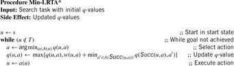
LRTA* needs to predict the successor states of actions (i.e., the successor states resulting from their execution). We can decrease its lookahead further if we associate the values with state-action pairs rather than states. Algorithm 11.4 shows pseudo code for Min-LRTA*, which associates a q-value  with each action
  that can be executed in state
  . The q-values are similar to the signs used by SLRTA* and the state-action values of reinforcement-learning methods, such a Q-Learning, and correspond to the costs-to-go of the actions. The q-values are updated as the search progresses, both to focus the search and avoid cycling. Min-LRTA* has minimal lookahead (essentially lookahead zero) because it uses only the q-values local to the current state to determine which action to execute. Thus, it does not even project one action execution ahead. This means that it does not need to learn an action model of the state space, which makes it applicable to situations where the action model is not known in advance, and thus the agent cannot predict the successor states of actions before it has executed them at least once. The action-selection step of Min-LRTA* always greedily chooses an action with the minimal q-value in the current state. The value-update step of Min-LRTA* replaces
  with a more accurate lookahead value. This can be explained as follows: The q-value
  of any state-action pair is the cost-to-go of action a′ in state v and thus a lower bound on the goal distance if one starts in state v, executes action a′, and then behaves optimally. Thus,
  is a lower bound on the goal distance of state v, and
  is a lower bound on the goal distance if one starts in state u, executes action a, and then behaves optimally. Min-LRTA* always reaches a goal state with a finite execution cost in all safely explorable state spaces, as can be shown with a cycle argument in a way similar to the proof of the same property of LRTA*.
Theorem 11.3
(Execution Cost of Real-Time Search with Minimal Lookahead) The complexity of every real-time search method that cannot predict the successor states of actions before it has executed them at least once is Ω (ed) over all state spaces where all action costs are one. Furthermore, the complexity is Ω (n3) over all reasonable state spaces where all action costs are one.
Proof
Figure 11.7 shows a complex state space, which is a reasonable state space in which all states (but the start state) have several actions that lead back toward the start state. All action costs are one. Every real-time search method that cannot predict the successor states of actions before it has executed them at least once has to execute Ω (ed) or, alternatively, Ω (n3) actions in the worst case to reach a goal state in complex state spaces. It has to execute each of the  actions in nongoal states that lead away from the goal state at least once in the worst case. Over all of these cases, it has to execute
  actions on average to recover from the action, for a total of
  actions. In particular, it can execute at least
  actions before it reaches the goal state (for
  ). Thus, the complexity is
  and
and  since
since  (for
(for  ) and
) and  (for
(for  ).
).
Theorem 11.3 provides lower bounds on the number of actions that zero-initialized Min-LRTA* executes. It turns out that these lower bounds are tight for zero-initialized Min-LRTA* over all state spaces where all action costs are one and remain tight over all undirected state spaces and Eulerian state spaces where all action costs are one (see Exercises).
11.5.3. Variants with Faster Value Updates
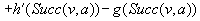
Real-time adaptive A* (RTAA*) is a real-time search method that is similar to LRTA* but its value-update step is much faster. Assume that we have to perform several (forward) A* searches with consistent h-values in the same state space and with the same set of goal states but possibly different start states. Assume that v is a state that was expanded during such an A* search. The distance from the start state s to any goal state via state v is equal to the distance from the start state s to state v plus the goal distance δ (v, T) of state v. It clearly cannot be smaller than the goal distance δ (s, T)of the start state s. Thus, the goal distance δ (v, T) of state v is no smaller than the goal distance δ (s, T) of the start state s(i.e., the f-value  of the goal state
  that was about to be expanded when the A* search terminates) minus the distance from the start state s to state v(i.e., the g-value g (v) of state v when the A* search terminates):
Consequently,  provides a nonoverestimating estimate of the goal distance δ (v, T) of state v and can be calculated quickly. More informed consistent h-values can be obtained by calculating and assigning this difference to every state that was expanded during the A* search and thus is in the closed list when the A* search terminates. We now use this idea to develop RTAA*, which reduces to the case above if its local search spaces are maximal.
Algorithm 11.5 shows pseudo code for RTAA*, which follows the pseudo code of LRTA*. The h-values of RTAA* approximate the goal distances of the states. They can be initialized using a consistent heuristic function. We mentioned earlier that LRTA* could use (forward) A* searches to determine the local search spaces. RTAA* does exactly that. The (forward) A* search in the pseudo code is a regular A* search that uses the current h-values to search from the current state of the agent toward the goal states until a goal state is about to be expanded or lookahead > 0 states have been expanded. After the A* search, we require  to be the state that was about to be expanded when the A* search terminated. We denote this state consistently with
  . We require that
  if the A* search terminated due to an empty open list, in which case it is impossible to reach a goal state with finite execution cost from the current state and RTAA* thus returns failure. Otherwise,
  is either a goal state or the state that the A* search would have been expanded as the (lookahead + 1) st state. We require the closed list Closed to contain the states expanded during the A* search and the g-value g (v) to be defined for all generated states v, including all expanded states. We define the f-values
  for these states v. The expanded states v form the local search space, and RTAA* updates their h-values by setting
  . The h-values of the other states remain unchanged. We give an example of the operation of RTAA* in Section 11.6.2. For example, consider Figure 11.16. The states in the closed list are shown in gray, and the arrows point to the states
  .
.
RTAA* always reaches a goal state with a finite execution cost in all safely explorable state spaces no matter how it chooses its values of lookahead and whether it uses the repeat-until loop or not, as can be shown with a cycle argument in a way similar to the proof of the same property of LRTA*. We now prove several additional properties of RTAA* without repeat-until loop. We make use of the following known properties of A* searches with consistent h-values. First, they expand every state at most once. Second, the g-values of every expanded state v and state  are equal to the distance from the start state to state v and state
  , respectively, when the A* search terminates. Thus, we know minimal-cost paths from the start state to all expanded states and state
  . Third, the f-values of the series of expanded states over time are monotonically nondecreasing. Thus,
  for all expanded states v and
  for all generated states v that remained unexpanded when the A* search terminates.
 |
| Figure 11.16 |
Lemma 11.4
Consistent initial h-values remain consistent after every value-update step of RTAA* and are monotonically nondecreasing.
Proof
We first show that the h-values are monotonically nondecreasing. Assume that the h-value of a state v is updated. Then, state v was expanded and it thus holds that  . Consequently,
  and the value-update step cannot decrease the h-value of state v since it changes the h-value from h (v) to
 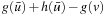 . We now show that the h-values remain consistent by induction on the number of A* searches. The initial h-values are provided by the user and consistent. It thus holds that
  for all goal states v. This continues to hold since goal states are not expanded and their h-values thus not updated. (Even if RTAA* updated the h-value of state
  , it would leave the h-value of that state unchanged since
  . Thus, the h-values of the goal states would remain zero even in that case.) It also holds that
  for all nongoal states v and actions a that can be executed in them, since the h-values are consistent. Let h denote the h-values before the value-update step and h′ denote the h-values after the value-update step. We distinguish three cases for all nongoal states v and actions a that can be executed in them:
• Second, state v was expanded but state  was not, which implies that
 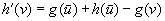 and
and  . Also,
  for the same reason as in the first case, and
 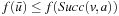 since state
  was generated but not expanded. Thus,


 .
.
• Third, state v was not expanded, which implies that  . Also,
  since the h-values of the same state are monotonically nondecreasing over time. Thus,
  .
.
Thus,  in all three cases and the h-values thus remain consistent.
Theorem 11.4
(Convergence of RTAA*) Assume that RTAA* maintains h-values across a series of search tasks in the same safely explorable state space with the same set of goal states. Then, the number of search tasks for which RTAA* with consistent initial h-values reaches a goal state with an execution cost of more than δ (s, T) (where s is the start state of the current search task) is bounded from above.
Proof
The proof is identical to the proof of Theorem 11.2, except for the part where we prove that the h-value of state v is set to its goal distance if the agent transitions from a state v of which the h-value is not equal to its goal distance to a state w of which the h-value is equal to its goal distance. When the agent executes some action  in state v and transitions to state w, then state v is a parent of state w in the search tree produced during the last call of A* and it thus holds that (1) state v was expanded during the last call of A*, (2) either state w was also expanded during the last call of A* or
  , and (3)
  . Let h denote the h-values before the value-update step and h′ denote the h-values after the value-update step. Then,
  and
and  . The last equality holds because we assumed that the h-value of state w was equal to its goal distance and thus can no longer change since it could only increase according to Lemma 11.4 but would then make the h-values inadmissible and thus inconsistent, which is impossible according to the same lemma. Consequently,
  , proving that
  since a larger h-value would make the h-values inadmissible and thus inconsistent, which is impossible according to Lemma 11.4. Thus, the h-value of state v is indeed set to its goal distance.
RTAA* and a variant of LRTA* that uses the same (forward) A* searches to determine the local search spaces differ only in how they update the h-values after the (forward) A* search. We now prove that LRTA* with minimal local search spaces and RTAA* with minimal local search spaces behave identically if they break ties in the same way. They can behave differently for larger local search spaces, and we give an informal argument why the h-values of LRTA* tend to be more informed than the ones of RTAA* with the same local search spaces. On the other hand, it takes LRTA* more time to update the h-values and it is more difficult to implement, for the following reason: LRTA* performs one search to determine the local search space and a second search (using the variant of Dijkstra's algorithm from Algorithm 11.2) to determine how to update the h-values of the states in the local search space since it is unable to use the results of the first search for this purpose. Thus, there is a trade-off between the search cost and the execution cost.
Theorem 11.5
Proof
We show the property by induction on the number of A* searches of RTAA*. The h-values of both search methods are initialized using the same heuristic function and are thus identical before the first A* search of RTAA*. Now consider any A* search of RTAA* and let  be the state that was about to be expanded when the A* search terminated. Let h denote the h-values of RTAA* before the value-update step and h′ denote the h-values after the value-update step. Similarly, let
  denote the h-values of LRTA* before the value-update step and
  denote the h-values after the value-update step. Assume that RTAA* and LRTA* are in the same state, break ties in the same way, and
  for all states v. We show that
  for all states v. Both search methods expand only the current state u of the agent and thus update only the h-value of this one state. It holds that
  and
and 
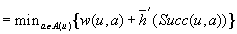


 , since the h-values of LRTA* remain consistent and are monotonically nondecreasing according to Lemma 11.2, which implies that
  for all
  . Thus, both search methods set the h-value of the current state to the same value and, if they break ties identically, then move to state
  . Consequently, they behave identically.
We now give an informal argument why the h-values of LRTA* with larger local search spaces tend to be more informed than the ones of RTAA* with the same local search spaces (if both real-time search methods execute the same number of actions after every search). This is not a proof but gives some insight into the behavior of the two search methods. Let h denote the h-values of RTAA* before the value-update step and h′ denote the h-values after the value-update step. Similarly, let  denote the h-values of LRTA* before the value-update step and
  denote the h-values after the value-update step. Assume that both search methods with consistent initial h-values are in the same state, break ties in the same way, and
  for all states v. We now prove that
  for all states v. The A* searches of both search methods are identical if they break ties in the same way. Thus, they expand the same states and thus also update the h-values of the same states. We now show that the h-values h′ cannot be consistent if
  for at least one state v, contradicting Lemma 11.4. Assume that
  for at least one state v. Pick a state v with the minimal
  for which
  and pick an action a with
  . State v must be a nongoal state and have been expanded since
  but
but  . Then, it holds that
  according to Lemma 11.1. Since
  and state v is a state with the minimal
  for which
  , it must be the case that
  . Put together, it holds that
  . This means that the h-values h′ are inconsistent but they remain consistent according to Lemma 11.4, which is a contradiction. Consequently, it holds that
  for all states v. However, this proof does not imply that the h-values of LRTA* always (weakly) dominate the ones of RTAA* since the search methods can move the agent to different states and then update the h-values of different states, but it suggests that the h-values of LRTA* with larger local search spaces tend to be more informed than the ones of RTAA* with the same local search spaces and thus that LRTA* tends to have a smaller execution cost than RTAA* with the same local search spaces (if both real-time search methods execute the same number of actions after every search).
11.5.4. Variants That Detect Convergence
We can modify LRTA* with admissible initial h-values to keep track of which h-values are already equal to the corresponding goal distances. For example, LRTA* could mark states so that a state is marked if and only if LRTA* knows that its h-value is equal to its goal distance, similar to the idea behind the proof of Theorem 11.2. Assume that LRTA* with minimal local search spaces maintains h-values and markings across a series of search tasks in the same safely explorable state space with the same set of goal states. Initially, only the goal states are marked. If several actions tie in the action-selection step and the execution of at least one of them results in a marked state (or if the execution of the only action results in a marked state), then LRTA* selects such an action for execution and marks its current state as well. The resulting variant of LRTA* then has the following properties: When a state is marked, its h-value is equal to its goal distance and then can no longer change. Once LRTA* reaches a marked state, it follows a minimal-cost path from there to a goal state and all states on that path are marked. If the start state of LRTA* is marked, then it follows a minimal-cost path to a goal state. If the start state of LRTA* is not marked, then it has marked one additional state by the time it reaches a goal state (see Exercises).
11.5.5. Variants That Speed Up Convergence
The convergence of LRTA* can be accelerated in different ways. For example, we can increase the sizes of its local search spaces. But we have several options even for LRTA* with minimal local search spaces:
• We can use LRTA* in abstractions of the state spaces (where clusters of states form meta-states), which effectively increases the sizes of its local search spaces.
• We can use more informed (but still admissible) initial h-values.
• We can weigh the h-values more heavily by using  instead of
  in the action-selection and value-update steps, for a constant
  , similar to weighted A*, which is what ϵ-LRTA* does (see Exercises).
• We can change LRTA* to backtrack to the previous state (if possible) rather than execute the action selected by the action-selection step if the value-update step increased the h-value of the current state, with the idea that the action-selection step in the previous state might then select a different action than previously, which is what SLA* does. (LRTA* could also use a learning quota and only backtrack after the sum of the increases of the h-values of a number of states are larger than the learning quota, which is what SLA*T does.)
There is also some speculation that the convergence of LRTA* can be accelerated in undirected state spaces if its action-selection step breaks ties toward successor states with minimal f-values rather than randomly or toward successor states with maximal f-values. Breaking ties toward successor states with minimal f-values is inspired by A*, which efficiently determines a minimal-cost path by always expanding a leaf of the search tree with the minimal f-value. If the g-values and h-values are perfectly informed (i.e., the g-value of each state is equal to its start distance and its h-value is equal to its goal distance), then the states with minimal f-values are exactly those on minimal-cost paths from the start state to a goal state. Thus, if LRTA* breaks ties toward successor states with minimal f-values, it breaks ties toward a minimal-cost path. If the g-values and h-values are not perfectly informed (the more common case), then LRTA* breaks ties toward what currently looks like a minimal-cost path.
To implement this tie-breaking criterion, LRTA* needs to maintain g-values. It can update the g-values in a way similar to how it updates the h-values, except that it uses the predecessor states instead of the successor states. Algorithm 11.6 shows pseudo code for the resulting variant of LRTA* with lookahead one: It executes actions with minimal cost-to-go and breaks ties toward actions of which the execution results in successor states with smaller f-values. FAst Learning and CONverging Search (FALCONS) implements this principle more consequently: It minimizes the f-value of the successor state and breaks ties toward actions with smaller costs-to-go. To understand why it breaks ties this way, consider g-values and h-values that are perfectly informed. In this case, all states on a minimal-cost path have the same (minimal) f-values and breaking ties toward actions with smaller costs-to-go ensures that FALCONS moves toward a goal state. Thus, while LRTA* focuses its h-value updates on what it believes to be a minimal-cost path from its current state to a goal state, FALCONS focuses its h-value updates on what it believes to be a minimal-cost path from the start state to a goal state. While LRTA* greedily tries to get quickly to a goal state, FALCONS greedily tries to get quickly to a minimal-cost path from the start state to a goal state and then follows the path, as shown in Figure 11.8. When it increases the g-value or h-value of a state on the path, then it might no longer consider the path to be a minimal-cost path from the start state to a goal state, and then again greedily tries to get quickly to a minimal-cost path from the start state to a goal state and then follows the path until it finally converges to a minimal-cost path from the start state to a goal state if it maintains its g-values and h-values across a series of search tasks in the same safely explorable state space with the same start state and set of goal states.
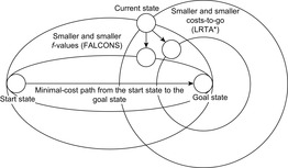
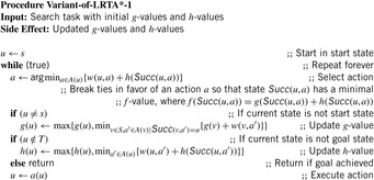

Algorithm 11.7 shows pseudo code for FALCONS. The initial g-values and h-values must be admissible (that is, they are lower bounds on the corresponding start and goal distances, respectively). We moved the termination-checking step after the value-update step because it makes sense to update the g-values in goal states. It turns out that care must be taken to ensure that FALCONS does not cycle forever and converges to a minimal-cost path from the start state to a goal state if it maintains its h-values across a series of search tasks in the same safely explorable state space with the same set of goal states, which explains why the value-update step is so complicated. The value-update step for the h-values, for example, basically simplifies to the one of LRTA* with lookahead one in case the h-values are consistent (see Exercises).
11.5.6. Nonconverging Variants
There are a large number of real-time search methods that basically operate like LRTA* but use h-values with different semantics and thus differ from LRTA* in their value-update steps, which allows them to reach a goal state but prevents them from converging if they maintain their h-values across a series of search tasks in the same safely explorable state space with the same set of goal states.
RTA*
A nonconverging variant of LRTA* is real-time A* (RTA*). Its h-values correspond to approximations of the goal distances of the states, just like the h-values of LRTA*. RTA* with lookahead one uses the value-update step but is otherwise identical to LRTA* with lookahead one. (The minimum of an empty set is infinity.) Thus, RTA* basically updates the h-value of the current state based on the cost-to-go of the second-best action, whereas LRTA* updates the h-value of the current state based on the cost-to-go of the best action. Thus, the h-values of RTA* do not necessarily remain admissible but the h-values of LRTA* do. RTA* always reaches a goal state with a finite execution cost in all safely explorable state spaces, as can be shown with a cycle argument in a way similar to the proof of the same property of LRTA*. Although RTA* applies to all safely explorable state spaces, the motivation for its value-update step comes from state spaces that are trees, where the only reason for entering the current state again is to execute the currently second-best action. (If we execute an action that enters the current state again and then execute the currently best action again, then these two actions together have no effect and thus do not need to get executed.) Consider, for example, the state space shown in Figure 11.9. All action costs are one. LRTA* with lookahead one and RTA* with lookahead one move east in the start state. Then, however, LRTA* can move west and east before it is forced to move east, whereas RTA* is forced to move east right away. In general, RTA* tends to have a smaller execution cost than LRTA* but does not converge if it maintains its h-values across a series of search tasks in the same safely explorable state space with the same set of goal states.
Node Counting
Another nonconverging variant of LRTA* is node counting. Its h-values correspond to the number of times the states have been visited. It does not make sense to initialize them with a heuristic function. Rather, they are initialized with zero. Node counting then uses the value-update step (because the current state has been visited one additional time) but is otherwise identical to LRTA* with lookahead one from Algorithm 11.3 in state spaces where all action costs are one. Node counting always reaches a goal state with a finite number of action executions and thus a finite execution cost in all safely explorable state spaces, as can be shown with a cycle argument in a way similar to the proof of the same property of LRTA*. We now analyze node counting in more detail and compare it to LRTA* in state spaces where all action costs are one. Theorem 11.1 implies that LRTA* always reaches a goal state with a finite execution cost in all safely explorable state spaces where all action costs are one. Furthermore, the complexity of zero-initialized LRTA* with minimal local search spaces is
  over all state spaces where all action costs are one and
  over all safely explorable state spaces where all action costs are one. It turns out that these complexities remain tight over all undirected state spaces and over all Eulerian state spaces where all action costs are one (see Exercises). The complexity of zero-initialized node counting is at least exponential in n over all state spaces where all action costs are one. Figure 11.10 is a reset state space, which is a reasonable state space in which all states (but the start state) have an action that eventually resets one to the start state. All action costs are one. Node counting needs a number of action executions in the worst case to reach a goal state in reset state spaces that is at least exponential in n. In particular, if node counting breaks ties in favor of successor states with smaller indices, then it executes
  actions before it reaches the goal state (for
  ). Thus, the complexity of zero-initialized node counting is at least exponential in n over all state spaces where all action costs are one. It turns out that the complexity of zero-initialized node counting is also at least exponential in (the square root of ) n even over all reasonable undirected state spaces where all action costs are one and over all reasonable Eulerian state spaces where all action costs are one, including (planar) undirected trees (see Exercises).
Thus, the complexity of zero-initialized LRTA* is smaller than the one of zero-initialized node counting in all of these cases. LRTA* has other advantages over node counting as well since it is able to use heuristic knowledge to guide its searches, can take action costs into account, allows for larger local search spaces, and converges if it maintains its h-values across a series of search tasks in the same safely explorable state space with the same set of goal states.
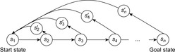
Edge Counting
Another nonconverging variant of LRTA* is edge counting, which relates to node counting as Min-LRTA* relates to LRTA*. Its q-values correspond to the number of times the actions have been executed. It does not make sense to initialize them with a heuristic function. Rather, they are initialized with zero. Edge counting then uses the value-update step but is otherwise identical to Min-LRTA* in state spaces where all action costs are one. The action-selection step of edge counting always chooses the action for execution that has been executed the least number of times. This achieves the same result as random walks (namely, to execute all actions in a state equally often in the long run), but in a deterministic way. One particular tie-breaking rule, for example, is for edge counting to repeatedly execute all actions in a state in turn according to a fixed order, resulting in edge ant walk. In other words, edge counting executes the first action according to the given order when it visits some state for the first time, it executes the second action according to the given order when it visits the same state the next time, and so on. Edge counting always reaches a goal state with a finite number of action executions and thus a finite execution cost in all safely explorable state spaces, as can be shown with a cycle argument in a way similar to the proof of the same property of LRTA*. The complexity of zero-initialized edge counting is at least exponential in n over all state spaces where all action costs are one (even over all reasonable state spaces where all action costs are one). Figure 11.11 is a variant of a reset state space, which is a reasonable state space in which all states (but the start state) have an action that resets one to the start state. All action costs are one. Edge counting needs a number of action executions in the worst case to reach a goal state in reset state spaces that is at least exponential in n. In particular, if edge counting breaks ties in favor of successor states with smaller indices, then it executes
  actions before it reaches the goal state (for
  ).
).
Thus, the complexity of zero-initialized Min-LRTA* is smaller than the one of zero-initialized edge counting over all state spaces where all action costs are one. However, it turns out that the complexity of zero-initialized edge counting is  over all undirected state spaces where all action costs are one and over all Eulerian state spaces where all action costs are one (see Exercises). Furthermore, its complexity is
  over all reasonable undirected state spaces where all action costs are one and over all reasonable Eulerian state spaces where all action costs are one. Thus, the complexity of zero-initialized Min-LRTA* is equal to the one of zero-initialized edge counting in these state spaces.
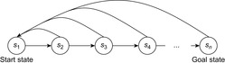 |
| Figure 11.11 Variant of reset state space, by Koenig and Simmons (1996). |
11.5.7. Variants for Nondeterministic and Probabilistic State Spaces
Search in nondeterministic and probabilistic state spaces is often more time consuming than search in deterministic state spaces since information limitations can only be overcome by enumerating all possible contingencies, which results in large search spaces. Consequently, it is even more important that agents take their search cost into account to solve search tasks efficiently. Real-time search in nondeterministic and probabilistic state spaces has an additional advantage compared to real-time search in deterministic state spaces, namely that it allows agents to gather information early. This information can be used to resolve some of the uncertainty and thus reduce the amount of search performed for unencountered situations. Without interleaving searches and action executions, an agent has to determine a complete conditional plan that solves the search task no matter which contingencies arise during its execution. Such a plan can be large. When interleaving searches and action executions, on the other hand, the agent does not need to plan for every possible contingency. It has to determine only the beginning of a complete plan. After the execution of this subplan, it can observe the resulting state and then repeat the process from the state that actually resulted from the execution of the subplan instead of all states that could have resulted from its execution, an advantage also exploited by game-playing programs.
Min-Max LRTA*
Min-max learning real-time A* (min-max LRTA*) uses minimax search to generalize LRTA* to nondeterministic state spaces. It views acting in nondeterministic state spaces as a two-player game in which it selects an action from the available actions in the current state. This action determines the possible successor states from which a fictitious agent, called nature, chooses one. Min-max LRTA* assumes that nature exhibits the most vicious behavior and always chooses the worst possible successor state.
Min-max LRTA* uses the maximal h-value of all successor states that can result from the execution of a given action in a given state everywhere in the pseudo code where LRTA* simply uses the h-value of the only successor state. Thus, the pseudo code of min-max LRTA* is identical to the pseudo code of LRTA* if every occurrence of  is replaced by
  in Algorithm 11.1, Algorithm 11.2, Algorithm 11.3 and Algorithm 11.8. For example, min-max LRTA* with lookahead one uses the action-selection step
 and the value-update step
 but is otherwise identical to LRTA* with lookahead one. Thus, min-max LRTA* is identical to LRTA* in deterministic state spaces. It turns out that min-max LRTA* has similar properties as LRTA* but the goal distance δ (u, T) of a state u now refers to its minimax goal distance; that is, the minimal execution cost with which a goal state can be reached from the state, even for the most vicious behavior of nature. For example, state spaces are now safely explorable if and only if the minimax goal distances of all states are finite and h-values are admissible if and only if they are lower bounds on the corresponding minimax goal distances. Then, Min-Max LRTA* with admissible initial h-values reaches a goal state with an execution cost of at most
  . Thus, it reaches a goal state with a finite execution cost in safely explorable state spaces.
The h-values of min-max LRTA* approximate the minimax goal distances of the states. (Informed) admissible h-values can be obtained as follows: We assume that nature decides in advance which successor state  to choose whenever action
  is executed in state
  ; all possible states are fine. If nature really behaved this way, then the state space would effectively be deterministic. h-values that are admissible for this deterministic state space are admissible for the nondeterministic state space as well. This is so because additional successor states allow a vicious nature to cause more harm. How informed the obtained h-values are in the nondeterministic state space depends on how informed they are in the deterministic state space and how close the assumed behavior of nature is to its most vicious behavior.
Assume that min-max LRTA* maintains h-values across a series of search tasks in the same safely explorable state space with the same set of goal states. It turns out that the number of search tasks for which min-max LRTA* with admissible initial h-values reaches a goal state with an execution cost that is larger than δ (s, T) (where s is the start state of the current search task) is bounded from above. The action sequences that min-max LRTA* executes after convergence if it maintains its h-values across a series of search tasks in the same safely explorable state space with the same set of goal states depend on the behavior of nature and are not necessarily uniquely determined, but their execution costs are at most as large as the minimax goal distance of the start state. Thus, the execution cost of min-max LRTA* is either worst-case optimal or better than worst-case optimal. This is possible because nature might not be as vicious as a minimax search assumes. Min-max LRTA* might not be able to detect the existence of a successor state with a large minimax goal distance by introspection since it does not perform a complete minimax search but partially relies on observing the actual successor states of actions, and nature can wait an arbitrarily long time to reveal its existence or choose not to reveal it at all. This can prevent the h-values of the encountered states from converging after a bounded execution cost (or bounded number of search tasks) and is the reason why we analyzed the behavior of LRTA* using the mistake-bounded error model, although this problem cannot occur for LRTA* if its action-selection step always breaks ties among the actions in the current state according to a fixed ordering of the actions. It is important to realize that, since min-max LRTA* relies on observing the actual successor states of actions it can have computational advantages even over several search episodes compared to a complete minimax search. This is the case if some successor states do not occur in practice since min-max LRTA* plans only for states that it actually encounters during its searches.
Probabilistic LRTA*
Min-max LRTA* assumes that nature chooses the successor state that is worst for the agent. The h-value of a node in the minimax search tree where it is the turn of nature to move is thus calculated as the maximum of the h-values of its children, and min-max LRTA* attempts to minimize the worst-case execution cost. One advantage of using min-max LRTA* is that it does not depend on assumptions about the behavior of nature. If min-max LRTA* reaches a goal state for the most vicious behavior of nature, it also reaches a goal state if nature uses a different and therefore less vicious behavior. However, the assumption that nature chooses the successor state that is worst for the agent is often too pessimistic and can make search tasks wrongly appear to be unsolvable, for example, if a vicious nature could force the agent to cycle forever no matter which actions the agent executes. In such situations, min-max LRTA* can be changed to assume that nature chooses the successor state according to a probability distribution that depends only on the current state and the executed action, resulting in a totally observable Markov decision process (MDP) problem. In this case, the h-value of a node in the probabilistic search tree where it is the turn of nature to move is calculated as the average of the h-values of its children weighted with the probability of their occurrence as specified by the probability distribution. Probabilistic LRTA*, this probabilistic variant of min-max LRTA*, then attempts to minimize the average execution cost rather than the worst-case execution cost. It uses the expected h-value of the successor states that can result from the execution of a given action in a given state everywhere in the pseudo code where LRTA* simply uses the h-value of the only successor state. Let  denote the probability with which the execution of action
  in state
  results in successor state
  . Then, the pseudo code of probabilistic LRTA* is identical to the pseudo code of LRTA* if every occurrence of
  is replaced by
 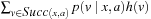 in Algorithm 11.2 and Algorithm 11.8. For example, probabilistic LRTA* with lookahead one uses the action-selection step
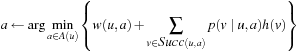 and the value-update step
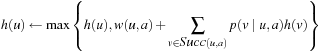 but is otherwise identical to LRTA* with lookahead one from Algorithm 11.3. However, the variant of Dijkstra's algorithm from Algorithm 11.2 cannot be used directly with the change since assigning each state in the local search space its new h-value requires the h-value of each state in the local search space to be updated multiple times. We can use value iteration, policy iteration, or other methods for solving MDPs for this purpose. Probabilistic LRTA* is identical to LRTA* in deterministic state spaces. It turns out that probabilistic LRTA* has similar properties as LRTA* but the goal distance of a state now refers to its expected goal distance. For example, state spaces are now safely explorable if and only if the expected goal distances of all states are finite, and h-values are admissible if and only if they are lower bounds on the corresponding expected goal distances.
11.6. How to Use Real-Time Search
We now discuss how to use real-time search using LRTA* as a basis. In addition to the case studies described in the following, real-time search methods have also been used in other nondeterministic state spaces from mobile robotics, including moving-target search, the task of catching moving prey.
11.6.1. Case Study: Offline Search
Many traditional state spaces from artificial intelligence are deterministic, including sliding-tile puzzles and blocks worlds. The successor states of actions can be predicted with certainty in deterministic state spaces. Real-time search methods can solve offline search tasks in these state spaces by moving a fictitious agent in the state space and thus provide alternatives to traditional search methods, such as A*. They have been applied successfully to traditional search tasks and Strips-type search tasks. For instance, real-time search methods easily determine suboptimal solutions for the Twenty-four Puzzle, a sliding-tile puzzle with more than 1024 states, and blocks worlds with more than 1027 states. For these search tasks, real-time search methods compete with other heuristic search methods such as greedy (best-first) search, which can determine suboptimal solutions faster than real-time search, or linear-space best-first search, which can consume less memory.
11.6.2. Case Study: Goal-Directed Navigation in A Priori Unknown Terrain
Goal-directed navigation in a priori unknown terrain requires a robot to move to a goal position in a priori unknown terrain. The robot knows the start and goal cell of the Gridworld but not which cells are blocked. It can repeatedly move one cell to the north, east, south, or west (unless that cell is blocked). All action costs are one. On-board sensors tell the robot in every cell which of the four adjacent cells (to the north, east, south, or west) are blocked. The task of the robot is to move to the given goal cell, which we assume to be possible. We study this search task again in Chapter 19. The robot uses a navigation strategy from robotics: It maintains the blockage status of the cells that it knows so far. It always moves along a presumed unblocked path from its current cell toward the goal cell until it visits the goal cell. A presumed unblocked path is a sequence of adjacent cells that does not contain cells that the robot knows to be blocked. The robot moves on the presumed unblocked path toward the goal cell but immediately repeats the process if it observes a blocked cell on the planned path or reaches the end of the path. Thus, it has to search repeatedly.
The states of the state space correspond to the cells, and the actions correspond to moving from a cell to an adjacent cell. The action costs can increase between searches. Initially, they are all one. When the robot observes that a cell is blocked, then it removes all actions that enter or leave the cell, which corresponds to setting their action costs to infinity. LRTA* and RTAA* apply to this scenario since consistent (or admissible) h-values remain consistent (or admissible, respectively) if action costs increase.
Figure 11.12 shows a simple goal-directed navigation task in a priori unknown terrain that we use to illustrate the behavior of repeated (forward) A* (that repeatedly searches from the current cell of the robot to the goal cell), LRTA* with repeat-until loop, and RTAA* with repeat-until loop. Black cells are blocked. All cells are labeled with their initial h-values, which are the Manhattan distances. All search methods start a new search episode (i.e., run another search) when the action cost of an action on their current path increases or, for LRTA* and RTAA*, when the new state is outside of their local search spaces, and break ties among cells with the same f-values in favor of cells with larger g-values and remaining ties in order from highest to lowest priority: east, south, west, and north. Figure 11.13, Figure 11.14, Figure 11.15 and Figure 11.16 show the robot as a small black circle. The arrows show the found paths from the current cell of the robot to the goal cell, which is in the bottom-right corner. Cells that the robot has already observed to be blocked are black. All other cells have their h-value in the bottom-left corner. Generated cells have their g-value in the top-left corner and their f-value in the top-right corner. Expanded cells are gray and, for RTAA* and LRTA*, have their updated h-values in the bottom-right corner, which makes it easy to compare them to the h-values before the update in the bottom-left corner.
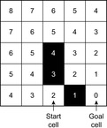 |
| Figure 11.12 |
 |
| Figure 11.13 |
 |
| Figure 11.14 |
 |
| Figure 11.15 |
Repeated (forward) A*, RTAA* with maximal local search spaces (i.e., with lookahead = ∞), and LRTA* with the same local search spaces follow the same paths if they break ties in the same way. They differ only in the number of cell expansions until the robot reaches the goal cell, which is larger for repeated (forward) A* (23) than for RTAA* with maximal local search spaces (20) and larger for RTAA* with maximal local search spaces (20) than for LRTA* with maximal local search spaces (19). The first property is due to RTAA* and LRTA* updating the h-values while repeated (forward) A* does not. Thus, repeated (forward) A* falls prey to the local minimum in the h-value surface and thus expands the three left-most cells in the bottom row a second time, whereas RTAA* and LRTA* avoid these cell expansions. The second property is due to some updated h-values of LRTA* being larger than the ones of RTAA*. However, most updated h-values are identical, although this is not guaranteed in general. We also compare RTAA* with lookahead = 4 to RTAA* with maximal local search spaces; that is, lookahead = ∞. Figures 11.14 and 11.16 show that smaller local search spaces increase the execution cost (from 10 to 12) but decrease the number of cell expansions (from 20 to 17) because smaller local search spaces imply that less information is used during each search episode. (The last search episode of RTAA* with lookahead = 4 expands only one cell since the goal cell is about to be expanded next.)
For goal-directed navigation in unknown terrain, smaller local search spaces tend to increase the execution cost of LRTA* and RTAA* but initially tend to decrease the number of cell expansions and the search cost. Increasing the execution cost tends to increase the number of search episodes. As the local search spaces become smaller, eventually the rate with which the number of search episodes increases tends to be larger than the rate with which the lookahead and the time per search episode decrease, so that the number of cell expansions and the search cost increase again. The number of cell expansions and the search cost tend to be larger for repeated (forward) A* than RTAA*, and larger for RTAA* than LRTA*. RTAA* with local search spaces that are neither minimal nor maximal tends to increase the h-values less per update than LRTA* with the same local search spaces. Consequently, its execution cost and number of cell expansions tend to be larger than the ones of LRTA* with the same local search spaces. However, it tends to update the h-values much faster than LRTA* with the same local search spaces, resulting in smaller search costs. Overall, the execution cost of RTAA* tends to be smaller than the one of LRTA* for given time limits per search episode because it tends to update the h-values much faster than LRTA*, which allows it to use larger local search spaces and overcompensate for its slightly less informed h-values.
11.6.3. Case Study: Coverage
Coverage requires a robot to visit each location in its terrain once or repeatedly. Consider a strongly connected state space without any goal states. Strongly connected state spaces guarantee that real-time search methods are always able to reach all states no matter which actions they have executed in the past. Then, LRTA* with lookahead one, RTA* with lookahead one, and node counting visit all states repeatedly, as can be shown with a cycle argument in a way similar to the proof that LRTA* always reaches a goal state with a finite execution cost. In fact, the worst-case cover time (where the cover time is measured as the execution cost until all states have been visited at least once) is the same as the worst-case execution cost until a goal state has been reached if an adversary can pick the goal state, for example, the state that was visited last when covering the state space. Thus, the earlier complexity results carry over to coverage.
The property of real-time search methods to visit all states of strongly connected state spaces repeatedly has been used to build ant robots —simple robots with limited sensing and computational capabilities. Ant robots have the advantage that they are easy to program and cheap to build. This makes it feasible to deploy groups of ant robots and take advantage of the resulting fault tolerance and parallelism. Ant robots cannot use conventional search methods due to their limited sensing and computational capabilities. To overcome these limitations, ant robots can use real-time search methods to leave markings in the state space that can be read by the other ant robots, similar to what real ants do when they use chemical (pheromone) traces to guide their navigation. For example, ant robots that all use LRTA* only have to sense the markings (in form of the h-values) of their adjacent states, and change the marking of their current state. They cover all states once or repeatedly even if they move asynchronously, do not communicate with each other except via the markings, do not have any kind of memory, do not know and cannot learn the topology of the state space, nor determine complete paths. The ant robots do not even need to be localized, which completely eliminates solving difficult and time-consuming localization tasks, and robustly cover all states even if they are moved without realizing that they have been moved (say, by people running into them), some ant robots fail, and some markings get destroyed.
Many of the real-time search methods discussed in this chapter could be used to implement ant robots. For example, the following properties are known if edge counting is used to implement ant robots, in addition to it executing all actions repeatedly. A Eulerian cycle is a sequence of action executions that executes each action in each state exactly once and returns to the start state. Consider edge ant walk, the variant of edge counting that repeatedly executes all actions in a state in turn according to a fixed order. In other words, edge counting executes the first action according to the given order when it visits some state for the first time, it executes the second action according to the given order when it visits the same state next time, and so on. It turns out that this variant of edge counting repeatedly executes a Eulerian cycle after at most  action executions in Eulerian state spaces without goal states, where the diameter d′ of a state space is the maximal distance between any pair of its states. Furthermore, consider k ant robots that each execute one action in each time step so that they repeatedly execute all actions in a state in turn according to a fixed order. In other words, the first ant robot that executes an action in some state executes the first action according to the given order, the next ant robot that executes an action in the same state executes the second action according to the given order, and so on. It turns out that the numbers of times that any two actions have been executed differ by at most a factor of two after at most
  time steps in Eulerian state spaces without goal states.
Overall, it is probably easiest to use node counting to implement ant robots in Gridworlds since each ant robot then marks cells and always increases the h-value of its current cell by the same amount. Figure 11.17 shows a simplified example. Each ant robot can repeatedly move one cell to the north, east, south, or west (unless that cell is blocked). We assume that there is no uncertainty in actuation and sensing. The ant robots move in a given sequential order (although this is not necessary in general). If a cell contains an ant robot, one of its corners is marked. Different corners represent different ant robots. Figure 11.17 (top) demonstrates how a single ant robot covers the Gridworld, and Figure 11.17 (bottom) demonstrates how three ant robots cover it. Ant robots that leave more information in each cell (e.g., complete maps) tend to cover terrain even faster.
 |
| Figure 11.17 |
11.6.4. Case Study: Localization and Goal-Directed Navigation under Pose Uncertainty
Consider the goal-directed navigation task with pose uncertainty shown in Figure 11.18. The robot knows the Gridworld, but is uncertain about its start pose, where a pose is a cell and orientation (north, east, south, or west). It can move one cell forward (unless that cell is blocked), turn left 90 degrees, or turn right 90 degrees. All action costs are one. On-board sensors tell the robot in every pose which of the four adjacent cells (front, left, behind, or right) are blocked. We assume that there is no uncertainty in actuation and sensing, and consider two navigation tasks. Localization requires the robot to gain certainty about its pose and then stop. We study this search task again in Chapter 19. Goal-directed navigation with pose uncertainty requires the robot to navigate to any of the given goal poses and then stop. Since there might be many poses that produce the same sensor reports as the goal poses, this navigation task includes localizing the robot sufficiently so that it knows that it is in a goal pose when it stops. We require that the Gridworlds be strongly connected (every pose can be reached from every other pose) and not completely symmetrical (localization is possible). This modest assumption makes all robot navigation tasks solvable, since the robot can always first localize itself and then, for goal-directed navigation tasks with pose uncertainty, move to a goal pose.
 |
| Figure 11.18 |
We now formally describe the navigation tasks, using the following notation: P is the finite set of possible robot poses. A (p) is the finite set of possible actions that the robot can execute in pose  : left, right, and possibly forward.
  is the pose that results from the execution of action
  in pose
  .
.  is the observation that the robot makes in pose
  : whether or not there are blocked cells immediately adjacent to it in the four directions (front, left, behind, and right). The robot starts in pose
  and then repeatedly makes an observation and executes an action until it decides to stop. It knows the Gridworld, but is uncertain about its start pose. It could be in any pose in
  . We require only that
  for all
  , which automatically holds after the first observation, and
  , which automatically holds for
  .
.
Since the robot does not know its start pose, the navigation tasks cannot be formulated as search tasks in small deterministic state spaces of which the states are the poses (pose space). Rather, the robot has to maintain a belief about its current pose. Analytical results about the execution cost of search methods are often about their worst-case execution cost (here, the execution cost for the worst possible start pose) rather than their average-case execution cost, especially if the robot cannot associate probabilities or other likelihood estimates with the poses. Then, all it can do is maintain a belief in the form of a set of possible poses, namely the poses that it could possibly be in. Thus, its beliefs are sets of poses and their number could be exponential in the number of poses. The beliefs of the robot depend on its observations, which the robot cannot predict with certainty since it is uncertain about its pose. For example, it cannot predict whether the cell in front of it will be blocked after it moves forward for the goal-directed navigation task with pose uncertainty from Figure 11.18. The navigation tasks are therefore search tasks in large nondeterministic state spaces of which the states are the beliefs of the robot (belief space). The robot will usually be uncertain about its current pose but can always determine its current belief for sure. For example, if the robot has no knowledge of its start pose for the goal-directed navigation task with pose uncertainty from Figure 11.18 but observes blocked cells all around it except in its front, then its start belief contains the following seven poses: A 1 →, A 6 ↓, A 8 ↓, A 10 →, D 1 →, D 5 ↑, and D 8 ↑.
We now formally describe the state spaces of the navigation tasks, using the following notation: B denotes the set of beliefs and b (s) the start belief. A (b) denotes the set of actions that can be executed when the belief is b.  denotes the set of possible observations that can be made after the execution of action a when the belief was b.
  denotes the successor belief that results if observation o is made after the execution of action a when the belief was b. Then, for all
  ,
,  , and
, and  ,
,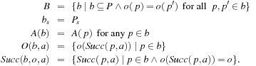
To understand the definition of A (b), notice that  for all
  after the preceding observation since the observation determines the actions that can be executed.
For goal-directed navigation tasks with pose uncertainty, the robot has to navigate to any pose in  and stop. In this case, we define the set of goal beliefs as
  . To understand this definition, notice that the robot knows that it is in a goal pose if and only if its belief is
  . If the belief contains more than one pose, however, the robot does not know which goal pose it is in. If it is important that the robot knows which goal pose it is in, we use
  . For localization tasks, we use
  .
.
The belief space is then defined as follows. It is safely explorable since our assumptions imply that all navigation tasks are solvable: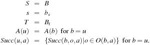
For goal-directed navigation tasks with pose uncertainty, we can use the admissible goal-distance heuristic,  . (Thus, the robot determines for each pose in the belief state how many actions it would have to execute to reach a goal pose if it knew that it was currently in that pose. The maximum of these values then is an approximation of the minimax goal distance of the belief state.) For example, the goal-distance heuristic is 18 for the start belief state used earlier, namely the maximum of 18 for A 1 →, 12 for A 6 ↓, 10 for A 8 ↓, 1 for A 10 →, 17 for D 1 →, 12 for D 5 ↑, and 9 for D 8 ↑. The calculation of
  involves no pose uncertainty and can be done efficiently without interleaving searches and action executions, by using traditional search methods in the pose space. This is possible because the pose space is deterministic and small. The h-values are admissible because the robot needs an execution cost of at least
  in the worst case to solve the goal-directed navigation task with pose uncertainty from pose
  , even if it knows that it starts in that pose. The h-values are often only partially informed because they do not take into account that the robot might not know its pose and then might have to execute additional localization actions to overcome its pose uncertainty. For localization tasks, on the other hand, it is difficult to obtain more informed initial h-values than zero-initialized ones.
Figure 11.19 (excluding the dashed part) shows how min-max LRTA* with lookahead one performs a minimax search around the current belief state of the robot to determine which action to execute next. The local search space consists of all nonleaves of the minimax tree where it is the robot's turn to move (labeled “Agent” in the figure). Min-max LRTA* first assigns all leaves of the minimax tree the h-value determined by the heuristic function for the corresponding belief state . Min-max LRTA* then backs up these h-values toward the root of the minimax tree. The h-value of a node in the minimax tree where it is nature's turn to move (labeled “Nature” in the figure) is the maximum of the h-values of its children since nature chooses successor states that maximize the minimax goal distance ②. The h-value of a node in the minimax search tree where it is the robot's turn to move is the maximum of its previous h-value and the minimum over all actions in the node of the sum of the action cost plus the h-value of the corresponding child since min-max LRTA* chooses actions that minimize the minimax cost-to-go . Finally, min-max LRTA* selects the action in the root that minimizes the sum of the action cost plus the h-value of the corresponding child. Consequently, it decides to move forward. Min-max LRTA* then executes the selected action (possibly already searching for action sequences in response to the possible observations it can make next), makes an observation, updates the belief state of the robot based on this observation, and repeats the process from the new belief state of the robot until the navigation task is solved.
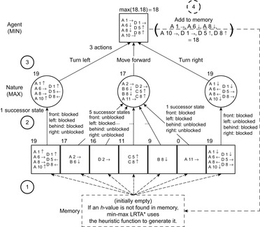 |
| Figure 11.19 Illustration of min-max LRTA*, by Koenig (2001). |
Min-max LRTA* has to ensure that it does not cycle forever. It can use one of the following two approaches to gain information between action executions and thus guarantee progress:
Direct Information Gain: If min-max LRTA* uses sufficiently large local search spaces, then it achieves a gain in information in the following sense. After executing the selected actions it is guaranteed that the robot has either solved the navigation task or at least reduced the number of poses it can be in. This way, it guarantees progress toward a solution. For example, moving forward reduces the number of possible poses from seven to at most two for the goal-directed navigation task with pose uncertainty from Figure 11.18. We study a search method with direct information gain, called greedy localization, in more detail in Chapter 19 since it performs agent-centered search but not real-time search.
Indirect Information Gain: Min-max LRTA* with direct information gain does not apply to all search tasks. Even if it applies, the local search spaces and thus the search cost that it needs to guarantee a direct information gain can be large. To operate with smaller local search spaces, it can use real-time search. It then operates as before, with the following two changes. First, when min-max LRTA* needs the h-value of a belief state just outside of the local search space (i.e., the h-value of a leaf of the minimax tree) in the value-update step, it now checks first whether it has already stored an h-value for this belief state in memory. If so, then it uses this h-value. If not, then it calculates the h-value using the heuristic function, as before. Second, after min-max LRTA* has calculated the h-value of a belief state in the local search space where it is the turn of the robot to move, it now stores it in memory, overwriting any existing h-value of the corresponding belief state. Figure 11.19 (including the dashed part) summarizes the steps of min-max LRTA* with indirect information gain before it decides to move forward. The increase of the potential  , see the proof of Lemma 11.3, can be interpreted as an indirect information gain that guarantees that min-max LRTA* reaches a goal belief state in safely explorable state spaces. A disadvantage of min-max LRTA* with indirect information gain over min-max LRTA* with direct information gain is that the robot has to store potentially one h-value in memory for each belief state it has encountered during its searches. In practice, however, the memory requirements of real-time search methods often seem to be small, especially if the initial h-values are well informed and thus focus the searches well, which prevents them from encountering a large number of different belief states. Furthermore, real-time search methods only need to store the h-values of those belief states in memory that differ from the initial h-values. If the h-values are the same, then they can be automatically regenerated when they are not found in memory. For the example from Figure 11.19, for instance, it is unnecessary to store the calculated h-value 18 of the start belief state in memory.
An advantage of min-max LRTA* with indirect information gain over min-max LRTA* with direct information gain is that it is able to operate with smaller local search spaces, even local search spaces that contain only the current belief state. Another advantage is that it improves its worst-case execution cost, although not necessarily monotonically, until it converges if it maintains its h-values across a series of localization tasks in the same terrain or goal-directed navigation tasks with pose uncertainty with the same set of goal poses in the same terrain. The actual start poses or the beliefs of the robot about its start poses do not need to be identical.
So far, we have assumed that the robot can recover from the execution of each action. If this is not the case, then the robot has to guarantee that the execution of each action does not make it impossible to reach a goal belief state, which is often possible by increasing the local search spaces of real-time search methods. For example, if min-max LRTA* is applied to goal-directed navigation tasks with pose uncertainty in the presence of irreversible actions and always executes actions so that the resulting belief state is guaranteed to contain either only goal poses, only poses that are part of the current belief state of the robot, or only poses that are part of the start belief state, then either the goal-directed navigation task remains solvable in the worst case or it was not solvable in the worst case to begin with. We have also assumed that there is no actuator or sensor noise. Search tasks with actuator but no sensor noise can be modeled with MDPs, and search tasks with actuator and sensor noise can be modeled with partially observable MDPs (POMDPs). We have already shown that MDPs can be solved with probabilistic LRTA*. A POMDP can be expressed as an MDP of which the state space is the set of probability distributions over all states of the POMDP. Thus, the state space of the resulting MDP is continuous and needs to get discretized before we can use probabilistic LRTA* on it.
11.7. Summary
In this chapter, we illustrated the concept of real-time search, described which kinds of search tasks it is suitable for, and discussed the design and the properties of some real-time search methods. We learned that real-time search methods have been applied to a variety of search tasks, including traditional off-line search, Strips-type planning, moving-target search, search of MDPs and POMDPs, reinforcement learning, and robot navigation (such as goal-directed navigation in unknown terrain, coverage and localization). We learned that real-time search methods have several advantages. First, different from the many existing ad hoc search and planning methods that interleave searches and action executions, they have a solid theoretical foundation and are state space independent. Second, they allow for fine-grained control over how much search to do between action executions. Third, they can use heuristic knowledge to guide their search, which can reduce the search cost without increasing the execution cost. Fourth, they can be interrupted at any state and resume execution at a different state. In other words, other control programs can take over control at arbitrary times if desired. Fifth, they amortize learning over several search episodes, which allows them to determine a solution with a suboptimal execution cost fast and then improve the execution cost as they solve similar search tasks, until the execution cost is satisficing or optimal. Thus, they still asymptotically minimize the execution cost in the long run in case similar search tasks unexpectedly repeat. Sixth, several agents can often solve search tasks cooperatively by performing an individual real-time search each but sharing the search information, thereby reducing the execution cost. For example, off-line search tasks can be solved on several processors in parallel by running a real-time search method on each processor and letting all real-time search methods share their h-values.
Although these properties can make real-time search methods the search methods of choice, we also learned that they are not appropriate for every search task. For example, real-time search methods execute actions before their consequences are completely known and thus cannot guarantee a small execution cost when they solve a search task for the first time. If a small execution cost is important, we might have to perform complete searches before starting to execute actions. Furthermore, real-time search methods trade off the search and execution costs but do not reason about the trade-off explicitly. In particular, it can sometimes be beneficial to update h-values of states that are far away from the current state, and repeated forward searches might not be able to determine these states efficiently. Time-bounded A*, for example, performs only one complete (forward) A* search and executes actions greedily until this search is complete. Finally, real-time search methods have to store an h-value in memory for each state encountered during their searches and thus can have large memory requirements if the initial h-values do not focus their searches well.
Table 11.1 provides an overview of the real-time search methods introduced in this chapter, together with the kind of their state spaces, the sizes of their local search spaces, and whether they are complete and converge. We discussed LRTA* as a prototypical real-time search method and analyzed its properties, including its completeness, execution cost and convergence. We then discussed several variants of LRTA*, including variants with maximal local search spaces, minimal local search spaces, lookahead one (similar to minimal local search spaces) and lookahead zero (called minimal lookahead, where all information is local to the current state). We discussed variants of LRTA* that update their h-values faster than LRTA* (namely RTAA*), that detect convergence, that speed up convergence (including FALCONS) and that do not converge (including RTA*, node counting and edge counting). We also discussed variants of LRTA* for nondeterministic state spaces (min-max LRTA*) and probabilistic state spaces (probabilistic LRTA*).
| Real-Time Search Method | Algorithm | State Space | Spaces or Lookaheads | h-Values | Completeness | Convergence |
|---|---|---|---|---|---|---|
| LRTA* | 11.1/11.2 | deterministic | one to infinity | admissible | yes | yes |
| LRTA* with lookahead one | 11.3 | deterministic | one | admissible | yes | yes |
| Min-LRTA* | 11.4 | deterministic | zero | admissible | yes | yes |
| RTAA* | 11.5 | deterministic | one to infinity | consistent | yes | yes |
| FALCONS | 11.7 | deterministic | one | admissible | yes | yes |
| RTA* | — | deterministic | one (to infinity) | admissible | yes | no |
| Node counting | — | deterministic | one | zero | yes | no |
| Edge counting | — | deterministic | zero | zero | yes | no |
| Min-Max LRTA* | — | nondeterministic | one (to infinity) | admissible | yes | yes |
| Probabilistic LRTA* | — | probabilistic | one (to infinity) | admissible | yes | yes |
11.8. Exercises
11.1 Consider the following algorithm for solving the (n2 −1)-Puzzle: If  , then solve it by brute force. Otherwise, use a greedy method to put the first row and column into place, tile by tile, and then call the algorithm recursively to solve the remaining rows and columns. Show a greedy method that can put an additional tile in the first row or column into place without disturbing the tiles that it has already put into place, and that only needs a constant search time before the first action execution and between action executions. (It turns out that there exists a greedy method with this property so that the resulting algorithm solves the with at most
  action executions.)
11.2 List several similarities and differences of min-max LRTA* and the minimax search method used by game-playing programs.
11.3 Determine experimentally which value of lookahead minimizes the search cost (here: runtime) when using LRTA* to solve the Eight-Puzzle with the Manhattan distance on your computer if the local search spaces are generated by (forward) A* search until a goal state is about to be expanded or lookahead > 0 states have been expanded.
11.4
1. Simulate by hand LRTA* with lookahead one in the state space from Figure 11.20 where the initial h-values label the states. All action costs are one. Clearly, LRTA* with small local search spaces executes a large number of actions to escape from depressions in the h-value surface.
3. Implement all three real-time search methods and experimentally compare them in more realistic state spaces of your choice.
11.5 We could add the additional value-update step  between the value-update step and the action-execution step of LRTA* with lookahead one, with the idea to update the h-value of a state not only based on the h-values of its successor states but also on the h-value of one of its predecessor states. Explain why this is only a good idea if the initial h-values are inconsistent.
11.6 Assume that LRTA* with minimal local search spaces maintains h-values and markings across a series of search tasks in the same safely explorable state space with the same set of goal states. Initially, only the goal states are marked. If several actions tie in the action-selection step and the execution of at least one of them results in a marked state (or if the execution of the only action results in a marked state), then LRTA* selects such an action for execution and marks its current state as well. Prove the following properties of the resulting variant of LRTA* with initial admissible h-values:
1. When a state is marked, its h-value is equal to its goal distance and then can no longer change.
2. Once LRTA* reaches a marked state, it follows a minimal-cost path from there to a goal state and all states on that path are marked.
3. If the start state of LRTA* is not marked, then it has marked one additional state by the time it reaches a goal state.
11.7 Assume that LRTA* with admissible initial h-values (very infrequently) gets teleported to a state close to its current state when it executes an action. How does this change its properties?
1. Are its h-values guaranteed to remain admissible?
2. Is it guaranteed to reach a goal state in safely explorable state spaces?
3. Is it guaranteed to converge to a minimal-cost path if it maintains its h-values across a series of search tasks in the same safely explorable state space with the same set of goal states?
11.8 Prove Lemma 11.1 and Lemma 11.2.
11.9 Prove that the complexity of zero-initialized Min-LRTA* is  over all state spaces where all action costs are one, in a way similar to the corresponding proof for LRTA*. As an intermediate step, prove results for Min-LRTA* similar to Lemma 11.3 and Theorem 11.1.
11.10 How do Lemma 11.3 and Theorem 11.1 change for LRTA* with lookahead one if some actions in nongoal states leave the current state unchanged in state spaces where all action costs are one?
11.11 Prove that the complexity of both zero-initialized Min-LRTA* and zero-initialized edge counting is  over all undirected state spaces where all action costs are one and over all Eulerian state spaces where all action costs are one, using the undirected lollipop state space from Figure 11.21.
11.12 Prove that the complexity of zero-initialized node counting is at least exponential in n even over all reasonable undirected state spaces where all action costs are one and over all reasonable Eulerian state spaces where all action costs are one.
11.13 Zero-initialized edge counting and zero-initialized node counting are related in state spaces where all action costs are one. Consider any state space X and a state space Y that is derived from state space X by replacing each of its directed edges with two directed edges that are connected with an intermediate state. Figure 11.22 gives an example. Then, node counting in state space Y, edge counting in state space Y, and edge counting in state space X behave identically (if ties are broken identically). This means that node counting in state space Y and edge counting in state space Y execute the same number of actions, which is twice the number of actions that edge counting executes in state space X (since they have to execute two actions for every action that edge counting executes in state space X). Is there a similar relationship between LRTA* and Min-LRTA*?
11.14 Section 11.6.2 mentions several experimental results in its last paragraph. Implement repeated (forward) A*, LRTA*, and RTAA* for goal-directed navigation in unknown terrain and confirm or disconfirm these results.
11.15 It turns out that goal-directed navigation tasks in unknown terrain can be solved with fewer cell expansions with repeated forward A* (that repeatedly searches from the current cell of the robot to the goal cell) than repeated backward A* (that repeatedly searches from the goal cell to the current cell of the robot), where cells are blocked randomly, the h-values of both variants of A* are initialized with the Manhattan distances, and all cell expansions are counted until the robot reaches the goal cell. The difference is substantial even though the branching factor is the same in both directions. Explain this phenomenon and then perform experiments to support your hypothesis in a Gridworld where all action costs are one.
11.16 Implement a Gridworld with five ant robots that all start in the same cell and use LRTA* with lookahead one to cover the Gridworld repeatedly. All action costs are one. Test out different ideas for how to make the ant robots cover the Gridworld faster or more uniformly.
1. Can you make the ant robots cover the Gridworld faster or more uniformly by biasing them away from each other so that they spread out more quickly?
2. Can you make the ant robots cover the Gridworld faster or more uniformly by letting them all use node counting instead of LRTA*?
3. Do the experimental cover times of LRTA* and node counting reflect the difference in their complexities?
11.17 Prove variants of Lemma 11.3, Theorem 11.1 and Theorem 11.2 for the variant of LRTA* from Algorithm 11.8 that does not constrain the order in which the h-values of the states are updated, which is sometimes called trial-based real-time dynamic programming. We can view it as repeating the value-update step with different local search spaces (at least one of which contains the current state) before it executes the action-selection step.
11.18 Describe how we can obtain (informed) admissible h-values for Probabilistic LRTA*, where the h-values approximate the expected goal distances of the states.
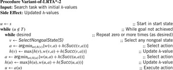
11.19 Consider one ant robot that performs an edge ant walk in the Gridworld from Figure 11.1 with the start cell given in the figure. How many action executions does it need in the worst case to visit every state of this undirected state space at least once (that is, for the worst possible order of actions in each state). How many action executions does it need in the worst case before it repeatedly executes a Eulerian cycle?
11.20 Consider LRTA* with lookahead one that uses  instead of
  in the action-selection and value-update steps, for a constant
  . Assume that this variant of LRTA* maintains h-values across a series of search tasks in the same safely explorable state space with the same set of goal states. Prove or disprove that the number of search tasks for which this variant of LRTA* with admissible initial h-values reaches a goal state with an execution cost that is larger than λ ⋅ δ (s, T) (where s is the start state of the current search task) is bounded from above.
11.21 The larger the sizes of the local search spaces of LRTA*, the smaller the execution cost of LRTA* tends to be. However, updating the h-values in larger local search spaces is time consuming. To run faster, LRTA* can update the h-values in its local search spaces only approximately, which is what RTAA* and the variant of LRTA* in Algorithm 11.8 do. There is also a variant of LRTA* that performs a branch-and-bound search, called minimin search, to set the h-value of the current state to the value calculated by our variant of Dijkstra's algorithm from Algorithm 11.2 but leaves the h-values of the other states in the local search space unchanged. In this general context, consider the variant of LRTA* from Algorithm 11.9. Initially, the non-negative h′-values are zero, and the s′-values are NULL. We use  as a shorthand for
  if
if  and
and  otherwise. (The minimum of an empty set is infinity.)
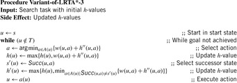
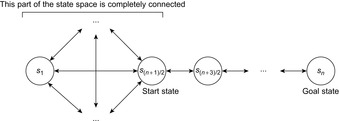 |
| Figure 11.21 Lollipop state space, by Koenig and Simmons (1996). |
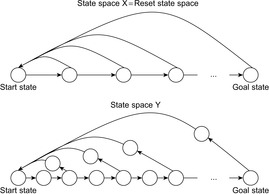
1. How does it relate to LRTA* with larger local search spaces?
2. How does it relate to RTA*?
3. Which properties does it have?
4. Can you improve on it?
11.22 Prove that edge counting always reaches a goal state with a finite number of action executions and thus finite execution cost in all safely explorable state spaces where all action costs are one.
11.23 Argue that Theorem 11.5 basically implies that the complexity results from Section 11.3 also apply to RTAA* with consistent initial h-values.
11.24 Simplify the value-update step of FALCONS in case its initial g-values and h-values are consistent.
11.25 The complexity of zero-initialized LRTA* with minimal local search spaces is  over all state spaces where all action costs are one and
  over all safely explorable state spaces where all action costs are one. Prove that these complexities remain tight over all undirected state spaces and Eulerian state spaces where all action costs are one. What are the corresponding complexities for RTAA*?
11.9. Bibliographic Notes
The term agent-centered search has been coined by Koenig (2001b); the term real-time heuristic search has been coined by Korf (1990); and the term trial-based real-time dynamic programming has been coined by Barto, Bradtke, and Singh (1995). Korf (1990) used real-time search originally for finding suboptimal solutions to large off-line search tasks, such as the Ninety-Nine-Puzzle.
Real-time search is related to pebble algorithms that agents can use to cover state spaces by marking otherwise indistinguishable states with colored pebbles (Blum Raghavan, and Schieber, 1991). Real-time search is also related to plan-envelope methods that operate on MDPs and, like Probabilistic LRTA*, reduce the search cost by searching only small local search spaces (plan envelopes). If the local search space is left during execution, then they repeat the process from the new state, until they reach a goal state (Dean, Kaelbling, Kirman, and Nicholson, 1995). However, they search all the way from the start state to a goal state, using local search spaces that usually border at least one goal state and are likely not to be left during execution. Finally, real-time search is also similar to reinforcement learning (see work by Thrun 1992 and Koenig and Simmons, 1996a) and to incremental search (see work by Koenig, 2004). Real-time search has been applied to traditional search tasks by Korf (1990) and Korf (1993); Strips-type planning tasks by Bonet, Loerincs, and Geffner 1997; moving-target search by Ishida (1997) and Koenig and Simmons (1995); coverage with ant robots by Wagner, Lindenbaum, andBruckstein (1999), Koenig, Szymanski, and Liu (2001a) and Svennebring and Koenig (2004); localization by Koenig (2001a); MDPs by Barto, Bradtke, and Singh (1995); and POMDPs by Bonet and Geffner (2000).
LRTA* has been described by Korf (1990) (including minimin search) and analyzed by Koenig (2001a); SLA* has been described by Shue and Zamani (1993); SLA*T has been described by Shue, Li, and Zamani (2001); ϵ-LRTA* has been described by Ishida (1997); RTAA* has been described by Koenig and Likhachev (2006); RTA* has been described by Korf (1990); node counting has been described by Koenig and Szymanski (1999) and has been analyzed by Koenig, Szymanski, and Liu (2001a); Min-LRTA* has been described by Koenig and Simmons (1996a); SLRTA* has been described by Edelkamp and Eckerle (1997); edge counting has been described by Koenig and Simmons (1996b); edge ant walk has been described by Yanovski, Wagner, and Bruckstein (2003); FALCONS has been described by Furcy and Koenig (2000); and min-max LRTA* has been described by Koenig (2001a).
Variants of LRTA* have been studied by Russell and Wefald (1991); variants of min-max LRTA* have been studied by Bonet and Geffner (2000) and Hernández and Meseguer (2005), Hernández and Meseguer (2007a) and Hernández and Meseguer (2007b); variants of node counting have been studied by Balch and Arkin (1993), Pirzadeh and Snyder (1990) and Thrun (1992); and variants of edge counting have been studied by Sutherland (1969). Improvements on these real-time search methods have been reported by Edelkamp and Eckerle (1997), Ishida (1997), Moore and Atkeson (1993), Pemberton and Korf (1992) and Pemberton and Korf (1994), Russell and Wefald (1991), Sutton (1991), Thorpe (1994) and Bulitko, Sturtevant, and Kazakevich (2005). Some of these improvements have been unified by Bulitko and Lee (2006).
Real-time search for cooperating agents other than ant robots has been studied by Ishida (1997), Knight (1993) and Felner, Shoshani, Altshuler, and Bruckstein (2006). A book-length overview on real-time search has been given by Ishida (1997) and covers many research results on real-time search by its author. Real-time search methods that do not satisfy our definition but only need a constant search time before the first action execution and between action executions, for example, have been described by Björnsson, Bultiko and Sturtevant (2009) for arbitrary state spaces (called time-bounded A*) and Parberry (1995) for sliding-tile puzzles.
..................Content has been hidden....................
You can't read the all page of ebook, please click here login for view all page.