
Chapter 6. Memory-Restricted Search
This chapter studies different algorithms that explore the middle ground between linear-space algorithms like IDA* and memory-sensitive algorithms like A*. It considers transposition tables for full and lossy/lossless sparse state set representations, as well as omission schemes for frontier and visited state sets.
Keywords: transposition table, fringe search, iterative threshold search, SMAG, enforced hill-climbing, weighted A, overconsistent A*, anytime repairing A*, k-best-first search, beam search, partial A*, partial IDA*, frontier search, sparse-memory graph search, breadth-first heuristic search, locality, beam-stack search, partial expansion A*, two-bit breadth-first search
In the previous chapter, we saw instances of search graphs, which were so large that they inherently call for algorithms capable of running under limited memory resources. So far, we have restricted the presentation to algorithms that consume memory that scales at most linear to the search depth. By the virtue of lower memory requirements, IDA* can solve problems that A* cannot. On the other hand, it cannot avoid revisiting nodes. Thus, there are many problems that neither A* nor IDA* can solve, because A* runs out of memory and IDA* takes too long. There have been several solutions being proposed to use the entire amount of main memory more effectively to store more information on potential duplicates. One problem of introducing memory for duplicate removal is a possible interaction with depth-bounded search. We observe an anomaly that goals are not found even if they have smaller costs than the imposed threshold.
We can coarsely classify the attempts by denoting whether or not they sacrifice completeness or optimality, and if they prune the Closed list, the Open list, or both. A broad class of algorithms that we focus on first uses all the memory that is available to temporarily store states in a cache. This reduces the number of reexpansions. We start with fixed-size hash tables in depth-bounded and iterative-deepening search. Next we consider memory-restricted state-caching algorithms that dynamically extend the search frontier. They have to decide which state to retain in memory and which one to delete.
If we are willing to sacrifice optimality or completeness, then there are algorithms that can obtain good solutions faster. This class includes exploration approaches that strengthen the influence of search heuristics in best-first searches and search algorithms that have limited coverage and look only at some parts of the search space. Approaches that are not optimal but are complete are useful mainly for overcoming inadmissibilities in the heuristic evaluation function and ones that sacrifice completeness.
Another class of algorithms reduces the set of expanded nodes, as full information might not be needed to avoid redundant work. Such a reduction is effective for problems that induce a small search frontier. In most cases, a regular structure of the search space (e.g., an undirected or acyclic graph structure) is assumed. As states on solution paths might no longer be present, after a goal has been found, the according paths have to be reconstructed.
The last class of algorithms applies a reduction to the set of search frontier nodes. The general assumption is that search frontier is large compared to the set of visited nodes. In some cases, the storage of all successors is avoided. Another important observation is that the breadth-first search frontier is smaller than the best-first search frontier, leading to cost-bounded BFS. We present algorithms closer to A* than to IDA*, which are not guaranteed to always find the optimal solution within the given memory limit, but significantly improve the memory requirements.
6.1. Linear Variants Using Additional Memory
A variety of algorithms have been proposed that are guaranteed to find optimal solutions, and that can exploit additionally available memory to reduce the number of expansions and hence the running time.
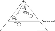
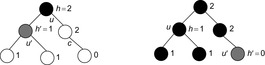
To emphasize the problems that can arise when introducing space for duplicate detection, let us introduce a Closed list in DFS. Unfortunately, bounding the depth to some value d (e.g., to improve some previously encountered goal) does not necessarily imply that every state reachable at a search depth less than d will eventually be visited. To see this, consider depth-bounded DFS as applied in the search tree of Figure 6.1.
The anomaly can be avoided by either reopening expanded nodes if reached on a smaller g-value or by applying an iterative-deepening strategy, which has searched for a low-cost solution before larger thresholds are applied. Table 6.1 shows the execution of such depth-first iterative-deepening exploration together with full duplicate detection for the example of Figure 2.1 (see also Figure 5.3 in Ch. 5).
| Step | Iteration | Selection | Open | Closed | U | U′ | Remarks |
|---|---|---|---|---|---|---|---|
| 1 | 1 | {} | {a} | {} | 0 | ∞ | |
| 2 | 1 | a | {} | {a} | 0 | 2 | g(b) |
| 3 | 2 | {} | {a} | {} | 2 | ∞ | New iteration starts |
| 4 | 2 | a | {b} | {a} | 2 | 6 | g(c) and g(d) > U |
| 5 | 2 | b | {} | {a, b} | 2 | 6 | |
| 6 | 3 | {} | {a} | {} | 6 | ∞ | New iteration starts |
| 7 | 3 | a | {b, c} | {a} | 6 | 10 | g(d) > U |
| 8 | 3 | b | {e, f, c} | {a, b} | 6 | 10 | |
| 9 | 3 | e | {f, c} | {a, b, e} | 6 | 10 | Duplicate |
| 10 | 3 | f | {c} | {a, b, e, f} | 6 | 10 | Duplicate |
| 11 | 3 | c | {} | {a, b, e, f, c} | 6 | 9 | g(d) |
| 12 | 4 | {} | {a} | {} | 9 | ∞ | New iteration starts |
| 13 | 4 | a | {b, c} | {a} | 9 | 10 | g(d) > U |
| 14 | 4 | b | {e, f, c} | {a, b} | 9 | 10 | |
| 15 | 4 | e | {f, c} | {a, b, e} | 9 | 10 | Duplicate |
| 16 | 4 | f | {c} | {a, b, e, f} | 9 | 10 | Duplicate |
| 17 | 4 | c | {d} | {a, b, e, f, c} | 9 | 10 | d Duplicate |
| 18 | 4 | d | {} | {a, b, e, f, c} | 9 | 10 | |
| 19 | 5 | {} | {a} | {} | 10 | 1 | New iteration starts |
| 20 | 5 | a | {b, c, d} | {a} | 10 | ∞ | |
| 21 | 5 | b | {e, f, c, d} | {a, b} | 10 | ∞ | |
| 22 | 5 | e | {f, c, d} | {a, b, e} | 10 | 1 | Duplicate |
| 23 | 5 | f | {c, d} | {a, b, e, f} | 10 | 1 | Duplicate |
| 24 | 5 | c | {d} | {a, b, e, f, c} | 10 | ∞ | |
| 25 | 5 | d | {} | {a, b, e, f, c, d} | 10 | 14 | g(g) |
| 26 | 6 | {} | {a} | {} | 14 | ∞ | New iteration starts |
| 27 | 6 | a | {b, c, d} | {a} | 14 | ∞ | g(d) > U |
| 28 | 6 | b | {e, f, c, d} | {a, b} | 14 | ∞ | |
| 29 | 6 | e | {f, c, d} | {a, b, e} | 14 | ∞ | Duplicate |
| 30 | 6 | f | {c, d} | {a, b, e, f} | 14 | ∞ | Duplicate |
| 31 | 6 | c | {d} | {a, b, e, f, c} | 14 | ∞ | |
| 32 | 6 | d | {g} | {a, b, e, f, c, d} | 14 | ∞ | |
| 33 | 6 | g | {} | {a, b, e, f, c, d} | 14 | ∞ | Goal reached |
6.1.1. Transposition Tables
The storage technique of transposition tables is inherited from the domain of two-player games; the name stems from duplicate game positions that can be reached by performing the same moves in a different order. Especially for single-agent searches, the name transposition table is unfortunate as transposition tables are full-flexible dictionaries that detect duplicates, even if not generated by move transpositions.
At least for problems with fast successor generators (like the (n2 − 1)-Puzzle) the construction and maintenance of the generated search space can be a time-consuming task compared to depth-first search approaches like IDA*. Transposition tables implemented as hash dictionaries (see Ch. 3), preserve a high performance. They store visited states u together with a cost value H(u) that is updated during the search.
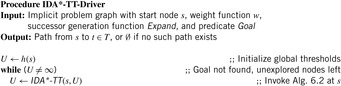
We present the use of transposition tables here as a variant of IDA* (compare Alg. 5.8 on page 205). We assume the implementation of a top-level driver routine (see Alg. 6.1), which matches the one of IDA* except that Closed is additionally initialized to the empty set. Furthermore, we see that Algorithm 6.2 returns the threshold U′ for the next iteration. Closed stores previously explored nodes u, together with a threshold H(u), such that the path costs from the root via u to a descendant of u is g(u) + H(u). Each newly generated node v is first tested against Closed; if this is the case, then the stored value H is a tighter bound than h(v).
The application of the algorithm to the example problem is shown in Table 6.2. We see that the (remaining) upper bound decreases. The approach applies one step less than the original IDA*, since node d is not considered twice.
| Step | Iteration | Selection | Open | Closed | U | U′ | Remarks |
|---|---|---|---|---|---|---|---|
| 1 | 1 | {} | {a} | {} | 11 | ∞ | h(a) |
| 2 | 1 | a | {} | {a} | 11 | 14 | b(b), b(c), and b(d) exceed U |
| 3 | 2 | {} | {a} | {(a, 14)} | 14 | ∞ | New iteration starts |
| 4 | 2 | a | {c} | {(a, 14)} | 14 | ∞ | b(b) and b(d) exceed U |
| 5 | 2 | c | {d} | {(a, 14)} | 8 | ∞ | b(a) exceeds U |
| 6 | 2 | d | {g} | {(a, 14)} | 5 | ∞ | b(a) exceeds U |
| 7 | 2 | g | {} | {(a, 14)} | 0 | Goal found |
Of course, if we store all expanded nodes in the transposition table, we would end up with the same memory requirement as A*, contrary to the original intent of IDA*. One solution to this problem is to embed a replacement strategy into the algorithm. One candidate would be to organize the table in the form of a first-in first-out queue. In the worst case, this will not provide any acceleration. By an adversary strategy argument, it may always happen that nodes just deleted are being requested.
Stochastic node caching can effectively reduce the number of revisits. While transposition tables always cache as many expanded nodes as possible, it stochastically caches expanded nodes. Whenever a node is expanded, we decide whether to keep the node in memory by flipping a (possibly biased) coin. This selective caching allows storing, with high probability, only nodes that are visited most frequently. The algorithm takes an additional parameter p, which is the probability of a node being cached every time it is expanded. It follows that the overall probability of a node being stored after it is expanded t times is 1 − (1 − p)t; the more frequent the same node is expanded, the higher the probability of it being cached becomes.
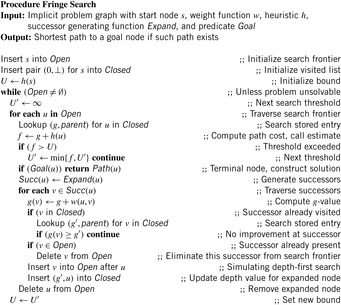
6.1.2. Fringe Search
Fringe search also reduces the number of revisits in IDA*. Regarded as a variant of A*, the key idea in fringe search is that Open does not need to be fully sorted, avoiding access to complex data structures. The essential property that guarantees optimal solutions is the same as in IDA*: A state with an f-value exceeding the largest f-value expanded so far must not be expanded, unless there is no state in Open with a smaller f-value.
Fringe search iterates over the frontier of the search tree. The data structure are two plain lists: Opent for the current iteration and Opent + 1 for the next iteration; Open0 is initialized with the initial node s and Open1 is initialized to the empty set.
Unless the goal is found the algorithm simulates IDA*. The first node u in Opent (head) is examined. If f(u) > U then u is removed from Open and inserted into Opent + 1 (at the end). Node u is only generated but not expanded in this iteration, so we save it for the next iteration. If f(u) ≤ U then we generate its successors and insert them into Opent (at the front), after which u is discarded. When a goal has not been found and the iteration completes, the search threshold is increased. Moreover, Opent + 1 becomes Opent, and Opent + 2 is set to empty. It is not difficult to see that fringe search expands nodes in the exact same order as IDA*.
Compared to A*, fringe search may visit nodes that are irrelevant for the current iteration, and A* must insert nodes into a priority queue structure (imposing some overhead). To the contrary, A*'s ordering means that it is more likely to find a goal sooner.
Algorithm 6.3 displays the pseudo code. The implementation is a little tricky, as it embeds Opent and Opent + 1 in one list structure. All nodes before the currently expanded nodes belong to the next search frontier in Opent + 1, whereas all nodes after the currently expanded nodes belong to the current search frontier Opent. Nodes u that are simply passed by executing the continue statement in case f(v) > U move from one list to the other. All other expanded nodes are deleted since they do not belong to the next search frontier. Successors are generated and checked whether or not they are duplicates of already expanded or generated nodes. If one matches a state, then the one with the best g-value (matches the f-value as the h-values are the same) will survive. If not refuted, the new state is inserted directly after the expanded nodes as still to be processed. The order of insertion is chosen such that the expansion order matches the depth-first strategy.
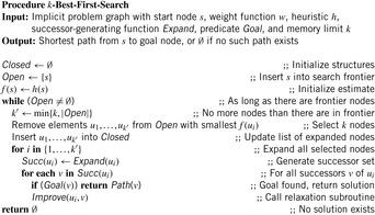
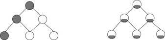
An illustration comparing fringe search (right) with IDA* (left) is given in Figure 6.2. The heuristic estimate is the distance to a leaf (height of the node). Both algorithms start with an initial threshold of h(s) = 3. Before the algorithm proves the problem to be unsolvable with a cost threshold of 3, two nodes are expanded and two nodes are generated. An expanded node has its children generated. A generated node is one where no search is performed because the f-value exceeds the threshold. In the next iteration, the threshold is increased to 4.
 |
| Figure 6.2 |
6.1.3. *Iterative Threshold Search
The memory-restricted iterative threshold search algorithm (ITS) also closely resembles that of IDA*. Similar to fringe search its exploration order is depth-first and not best-first. In contrast to fringe search, which assumes enough memory to be available and which does not need a complex data structure to support its search, ITS requires some tree data structure to retract nodes when running out of memory.
Compared to the previous approaches, ITS provides a strategy to replace elements in memory by their cost value. One particular feature is that it maintains information not only for nodes, but also for edges. The value f(u, v) stores a lower-bound estimate of a solution path using edge (u, v). Node v does not have to be generated—it suffices to know the operator leading to it without actually applying it. When a node u is created for the first time, all estimates f(u, v) are initialized to the usual bound f(u) = g(u) + h(u) (to deal with the special case that u has no successors, a dummy node d is assumed with f(u, d) = ∞; for brevity, this is not shown in the pseudo code). An edge (u, v), where v has not been created, is called a tip edge; a tip node is a node of which all outgoing edges are tip edges.
An implementation of the approach is shown in Algorithm 6.4 and Algorithm 6.5. The similarity of the algorithm to IDA* is slightly obscured by the fact that it is formulated in an iterative rather than recursive way; however, this alleviates its exposition. Note that IDA* uses a node ordering that is implicitly defined by the arbitrary but fixed sequence in which successors are generated. It is the same order that we refer to in the following when speaking, for example, of a left-most or right-most tip node.
As before, an upper threshold U bounds the depth-first search stage. The search tree is expanded until a solution is found, or all tip nodes exceed the threshold. Then the threshold is increased by the smallest possible increment to include a new edge, and a new iteration starts. If ITS is given no more memory than (plain) IDA*, every node generated by ITS is also generated by IDA*. However, when additional memory is available, ITS reduces the number of node expansions by storing part of the search tree and backing up heuristic values as more informed bounds.
The inner search loop always selects the left-most tip branch of which the f-value is at most U. The tail of the edge is expanded; that is, its g-value and f-value are computed, and its successor structures are initialized with this value. Finally, it is inserted into the search tree.
Global memory consumption is limited by a threshold maxMem. If this limit is reached, the algorithm first tries to select a node for deletion of which all the successor edges exceed the upper bound. From several such nodes, the left-most one with this condition is chosen. Otherwise, the right-most tip node is chosen. Before dropping the node, the minimum f-value over its successors is backed up to its parent to improve the latter one's estimate and hence reduce the number of necessary reexpansions. Thus, even though the actual nodes are deleted, the heuristic information gained from their expansion is saved.
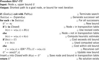
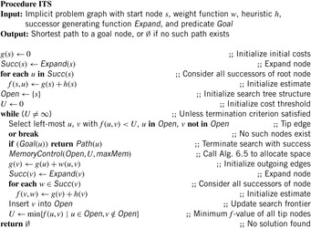
An example of a tree-structured problem graph for applying IDA* (top) and ITS (bottom) is provided in Figure 6.3. The tree is searched with the trivial heuristic (h ≡ 0). The initial node is the root and a single goal node is located at the bottom of the tree. After three iterations (left) all nodes in the top half of the search tree have been traversed by the algorithm. Since the edges to the left of the solution path have not led to a goal they are assigned to cost ∞. As a result, ITS avoids revisits of the nodes in the subtrees below. In contrast, IDA* will reexplore these nodes several times. In particular, in the last iteration (right), IDA* revisits several nodes of the top part.
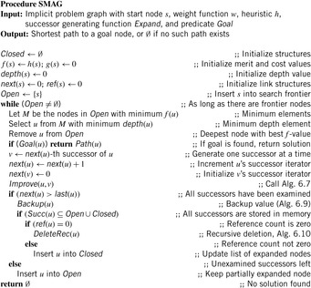
6.1.4. MA*, SMA, and SMAG
The original algorithm MA* underwent several improvements, during the course of which the name changed to SMA* and later to SMAG. We will restrict ourselves to describing the latter.
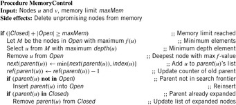
Contrary to A*, SMAG (see Alg. 6.6) generates one successor at a time. Compared to ITS, its cache decisions are based on problem graph nodes rather than on problem graph edges. Memory restoration is based on maintaining reference count(er)s. If a counter becomes 0, the node no longer needs to be stored. The algorithm assumes a fixed upper bound on the number of allocated edges in Open ∪ Closed. When this limit is reached, space is reassigned by dynamically deleting one previously expanded node at a time, and if necessary, moving its parent back to Open such that it can be regenerated. A least-promising node (i.e., one with the maximum f-value) is replaced. If there are several nodes with the same maximum f-value, then the shallowest one is taken. Nodes with the minimum f-value are selected for expansion; correspondingly, the tie-breaking rule prefers the deepest one in the search tree.
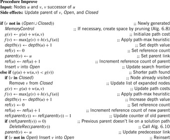
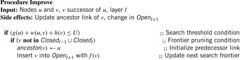
The update procedure Improve is shown in Algorithm 6.7. Here, reference counts and depth values are adapted. If the reference count (at some parent place) decreases to zero, a (possible recursive) node delete procedure for unused nodes is invoked. The working of the function is close to the one of a garbage collector for dynamic memory regions in some programming languages like Java. In the assignment to ref(parent(v)) nothing will happen if v is equal to the initial node s.
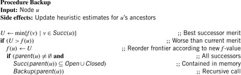
Thus, the Open list contains partially expanded nodes. It would be infeasible to keep track of all nodes storing pointers to all successors; instead we assume that each node keeps track of an iterator index next indicating the smallest unexamined child. The information about forgotten nodes is preserved by backing up the minimum f-value of descendants in a completely expanded subtree (see Alg. 6.9). Because f(u) is an estimate of the least-cost solution path through u, and the solution path is restricted to pass one of u's successors, we can obtain a better estimate from If all successors of u have been dropped, we will not know which way to go from u, but we still have an idea of how worthwhile it is to go anywhere from u. The backed-up values provide a more informed estimate.
When regenerating forgotten nodes, to reduce the number of repeated expansions we would also like to use the most informed estimate. Unfortunately, the estimates of individual paths are lost. One considerable improvement is the so-called path-max heuristic (as introduced in Sec. 2.2.1): If the heuristic is at least admissible, since a child's goal distance can only be smaller than the parent's by the edge cost, it is valid to apply the bound max{f(v), f(u)}, where v ∈ Succ(u).
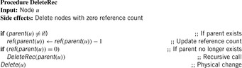
One complication of the algorithm is the need to prune a node from the Closed list if it does not occur on the best path to any fringe node. Since these nodes are essentially useless, they can cause memory leaks. The problem can be solved by introducing a reference counter for each node that keeps track of the number of successor nodes of which the parent pointer refers to them. When this count goes to zero, the node can be deleted; moreover, this might give rise to a chain of ancestor deletions as sketched in Algorithm 6.10.
Since the algorithm requires the selection of both the minimum and the maximum f-value, the implementation needs a refined data structure. For example, we could use two heaps or a balanced tree. To select a node according to its depth, a tree of trees could also be employed.
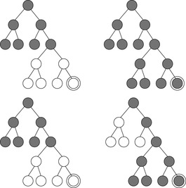
As an example of state generation in SMAG, we take a search tree with six nodes as shown in Figure 6.4. Let the memory limit be assigned to store at most three nodes. Initially, node a is stored in memory with a cost of 20, then nodes b and c are generated next with a costs of 30 and 25, respectively. Now a node has to be deleted to continue exploration. We take node c because it has the highest cost. Node a is annotated with a cost of 30, which is the lowest cost for a deleted child. Successor node d of node b is generated with a cost of 45. Since node d is not a solution it is deleted and node b is annotated with 45. The next child of b, node e, is then generated. Since node e is not a solution either, node e is deleted and node b is regenerated, because node b is the node with the next best cost. After node b is regenerated, node c is deleted, so that goal node f with zero cost is found.

6.2. Nonadmissible Search
In Section 2.2.1 we have seen that the use of an admissible heuristic guarantees that algorithm A* will find an optimal solution. However, as problem graphs are so huge, waiting for the algorithm to terminate becomes unacceptable, if regarding the limitation of main memory the algorithm can be carried out at all. Therefore, variants of heuristic search algorithms were developed that do not insist on the optimal solution, but a good solution in feasible time and space. Some strategies even sacrifice completeness and may fail to find a solution of a solvable problem instance. These algorithms usually come with strategies that decrease the likelihood of such errors. Moreover, they are able to obtain optimal solutions to problems where IDA* and A* fail.
6.2.1. Enforced Hill-Climbing
Hill-climbing is a greedy search engine that selects the best successor node under evaluation function h, and commits the search to it. Then the successor serves as the actual node, and the search continues. Of course, hill-climbing does not necessarily find optimal solutions. Moreover, it can be trapped in state space problem graphs with dead-ends. On the other hand, the method proves to be extremely efficient for some problems, especially the easiest ones.
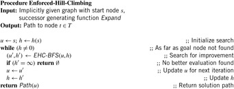
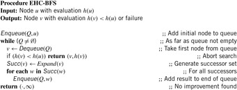
A more stable version is enforced hill-climbing. It picks a successor node, only if it has a strictly better evaluation than the current node. Since this node might not be in the immediate neighborhood of the current node, enforced hill-climbing searches for that node in a breadth-first manner. We have depicted the pseudo code for the driver in Algorithm 6.11. The BFS procedure is shown in Algorithm 6.12. We assume a proper heuristic with h(t) = 0, if and only if t is a goal. An example is provided in Figure 6.5.
Theorem 6.1
(Completeness Enforced Hill-Climbing) If the state space graph contains no dead-ends thenAlgorithm 6.12will find a solution.
Proof
There is only one case that the algorithm does not find a solution; that is, for some intermediate node v, no better evaluated node v can be found. Since BFS is a complete search method, it will find a node on a solution path with better evaluation. In fact, if it were not terminated in the case of h(v) < h(u), but in the case of h(v) = 0, it would find a full solution path.
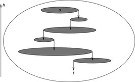
If we have an unweighted problem graph, then it contains no dead-ends. Moreover, any complete algorithm can be used instead of BFS. However, there is no performance guarantee on the solution path obtained. An illustration of the search plateaus generated by the enforced hill-climbing algorithm is provided in Figure 6.6. The plateaus do not have to be disjoint, as intermediate nodes in one layer can exceed the h-value for which the BFS search was invoked.
 |
| Figure 6.6 |
Besides being incomplete in directed graphs the algorithm has other drawbacks. There is evidence that when the heuristic estimation is not very accurate, enforced hill-climbing easily suffers from stagnation or is led astray.
6.2.2. Weighted A*
We often have that the heuristic h drastically underestimates the true distance, so that we can obtain a more realistic estimate by scaling up its influence with regard to some parameter. Although this compromises optimality, it can lead to a significant speedup; this is an appropriate choice when searching under time or space constraints.
If we parameterize  with
with  , we obtain a continuous range of best-first search variants Al, also denoted as weighted A*. For l = 0, we simulate a breadth-first traversal of the problem space; for l = 1, we have greedy best-first search. Algorithm A0.5 selects nodes in the same order as original A*.
If we choose l appropriately, the monotonicity of f is preserved.
Lemma 6.1
For l ≤ 0.5 and a consistent estimate h, fl is monotone.
Proof
Since h is consistent we have f monotone; that is, f(v) ≥ f(u) for all pairs (u, v) on a solution path. Consequently, since
since  .
.
Let us now relax the restrictions on l to obtain more efficient, though nonadmissible, algorithms. The quality of the solution can still be bounded in the following sense.
Definition 6.1
(ϵ-Optimality) A search algorithm is ϵ-optimal if it terminates with a solution of maximum cost  , with ϵ denoting an arbitrary small positive constant.
Lemma 6.2
A* where  for an admissible estimate h is ϵ-optimal.
Proof
For nodes u in Open that satisfy invariant (I) (Lemma 2.2) we have  and
and  due to the reweighting process. Therefore,
 Thus, if a node t ∈ T is selected we have
  .
.
ϵ-Optimality allows for more liberal selection of nodes for expansion.
Lemma 6.3
Let  . Then any selection of a node in Focal yields an ϵ-optimal algorithm.
Proof
Let u be the node in invariant (I) (Lemma 2.2) with  and let v be the node with the minimal f-value in Open. Then f(v) ≤ f(u), and for a goal t we have
  .
.
6.2.3. Overconsistent A*
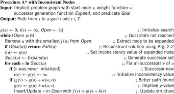
We can reformulate A* search to reuse the search results of its previous executions. To do this, we define the notion of an inconsistent node and then formulate A* search as the repeated expansion of inconsistent nodes. This formulation can reuse the results of previous executions simply by identifying all the nodes that are inconsistent.
We will first introduce a new variable, called i. Intuitively, these i-values will be estimates of start distances, just like g-values. However, although g(u) is always the cost of the best path found so far from s to u, i(u) will always be equal to the cost of the best path from s to u found at the time of the last expansion of u. If u has never been expanded then i(u) is set to ∞. Thus, every i-value is initially set to ∞ and then it is always reset to the g-value of the node when the node is expanded. The pseudo code of A* that maintains these i-values is given in Algorithm 6.13.
Since we set i(u) to g(u) at the beginning of the expansion of u and we assume nonnegative edge costs, i(u) remains equal to g(u) while u is being expanded. Therefore, setting g(v) to g(u) + w(u, v) is equivalent to setting g(v) to i(u) + w(u, v). As a result, one benefit of introducing i-values is the following invariant that A* always maintains: For every node v ∈ S, More importantly, however, it turns out that Open contains exactly all the nodes u visited by the search for which
  . This is the case initially, when all nodes except for s have both i- and g-values infinite and Open only contains s, which has i(s) = ∞ and g(s) = 0. Afterward, every time a node is being selected for expansion it is removed from Open and its i-value is set to its g-value on the very next line. Finally, whenever the g-value of any node is modified it has been decreased and is thus strictly less than the corresponding i-value. After each modification of the g-value, the node is made sure to be in Open.
(6.1)
Let us call a node u with  inconsistent and a node with i(u) = g(u) consistent. Thus, Open always contains exactly those nodes that are inconsistent. Consequently, since all the nodes for expansion are chosen from Open, A* search expands only inconsistent nodes.
An intuitive explanation of the operation of A* in terms of inconsistent node expansions is as follows. Since at the time of expansion a node is made consistent by setting its i-value equal to its g-value, a node becomes inconsistent as soon as its g-value is decreased and remains inconsistent until the next time the node is expanded. That is, suppose that a consistent node u is the best predecessor for some node v:  . Then, if g(u) decreases we get
  and therefore
  . In other words, the decrease in g(s) introduces an inconsistency between the g-value of u and the g-values of its successors. Whenever u is expanded, on the other hand, this inconsistency is corrected by reevaluating the g-values of the successors of u. This in turn makes the successors of u inconsistent. In this way the inconsistency is propagated to the children of u via a series of expansions. Eventually the children no longer rely on u, none of their g-values are lowered, and none of them are inserted into the Open list.
The operation of this new formulation of A* search is identical to the original version of A* search. The variable i just makes it easy for us to identify all the nodes that are inconsistent: These are all the nodes u with  . In fact, in this version of the subroutine, the g-values only decrease, and since the i-values are initially infinite, all inconsistent nodes have i(u) > g(u). We will call such nodes overconsistent, and nodes u with i(u) < g(u) are called underconsistent.
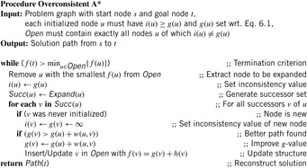
In the versions of A* just presented, all nodes had their g-values and i-values initialized at the outset. We set the i-values of all nodes to infinity, we set the g-values of all nodes except for s to infinity, and we set g(s) to 0. We now remove this initialization step and the only restriction we make is that no node is underconsistent and all g-values satisfy equation 6.1 except for g(s), which is equal to zero. This arbitrary overconsistent initialization will allow us to reuse previous search results when running multiple searches.
The pseudo code under this initialization is shown in Algorithm 6.14. The only change necessary for the arbitrary overconsistent initialization is the terminating condition of the while loop. For the sake of simplicity we assume a single goal node t ∈ T. The loop now terminates as soon as f(s) becomes less than or equal to the key of the node to be expanded next; that is, the smallest key in Open (we assume that the min operator on an empty set returns ∞). The reason for this addition is that under the new initialization t may never be expanded if it was already correctly initialized. For instance, if all nodes are initialized in such a way that all of them are consistent, then Open is initially empty, and the search terminates without a single expansion. This is correct, because when all nodes are consistent and g(s) = 0, then for every node u ≠ s,  , which means that the g-values are equal to the corresponding start distances and no search is necessary—the solution path from s to t is an optimal solution.
Just like the original A* search, for consistent heuristics, at the time the test of the while loop is being executed, for any node u with h(u) < ∞ and f(u) ≤ f(v) for all v in Open, it holds that the extracted solution path from u to t is optimal.
Given this property and the terminating condition of the algorithm, it is clear that after the algorithm terminates the returned solution is optimal. In addition, this property leads to the fact that no node is expanded more than once if heuristics are consistent: Once a node is expanded its g-value is optimal and can therefore never decrease afterward. Consequently, the node is never inserted into Open again. These properties are all similar to the ones A* search maintains. Different from A* search, however, the Improve function does not expand all the necessary nodes relevant to the computation of the shortest path. It does not expand the nodes of which the i-values were already equal to the corresponding start distances. This property can result in substantial computational savings when using it for repeated search. A node u is expanded at most once during the execution of the Improve function and only if i(u) was not equal to the start distance of u before invocation.
6.2.4. Anytime Repairing A*
In many domains A* search with inflated heuristics (i.e., A* search with f-values equal to g plus ϵ h-values for ϵ ≥ 1) can drastically reduce the number of nodes it has to examine before it produces a solution. While the path the search returns can be suboptimal, the search also provides a bound on the suboptimality, namely, the ϵ by which the heuristic is inflated. Thus, setting ϵ to 1 results in standard A* with an uninflated heuristic and the resulting path is guaranteed to be optimal. For ϵ > 1 the length of the found path is no larger than ϵ times the length of the optimal path, while the search can often be much faster than its version with uninflated heuristics.
To construct an anytime algorithm with suboptimality bounds, we could run a succession of these A* searches with decreasing inflation factors. This naive approach results in a series of solutions, each one with a suboptimality factor equal to the corresponding inflation factor. This approach has control over the suboptimality bound, but wastes a lot of computation since each search iteration duplicates most of the efforts of the previous searches. In the following we explain the ARA* (anytime repairing A*) algorithm, which is an efficient anytime heuristic search that also runs A* with inflated heuristics in succession but reuses search efforts from previous executions in such a way that the suboptimality bounds are still satisfied. As a result, a substantial speedup is achieved by not recomputing the node values that have been correctly computed in the previous iterations.
Anytime repairing A* works by executing A* multiple times starting with a large ϵ and decreasing ϵ prior to each execution until ϵ = 1. As a result, after each search a solution is guaranteed to be within a factor ϵ of optimal. ARA* uses the overconsistent A* subroutine to reuse the results of the previous searches and therefore can be drastically more efficient.
The only complication is that the heuristics inflated with ϵ may no longer be consistent. It turns out that the same function applies equally well when heuristics are inconsistent. Moreover, in general, when consistent heuristics are inflated the nodes in A* search may be reexpanded multiple times. However, if we restrict the expansions to no more than one per node, then A* search is still complete and possesses ϵ-suboptimality: the cost of the found solution is no worse than ϵ times the cost of an optimal solution.
The same holds true for the subroutine as well. We therefore restrict the expansions in the function (see Alg. 6.15) using the set Closed: Initially, Closed is empty; afterward, every node that is being expanded is added to it, and no node that is already in Closed is inserted into Open to be considered for expansion. Although this restricts the expansions to no more than one per node, Open may no longer contain all inconsistent nodes. In fact, Open contains only the inconsistent nodes that have not yet been expanded. We need, however, to keep track of all inconsistent nodes since they will be the starting points for the inconsistency propagation in the future search iterations. We do this by maintaining the set Incons of all the inconsistent nodes that are not in Open in Algorithm 6.15. Thus, the union of Incons and Open is exactly the set of all inconsistent nodes, and can be used to reset Open before each call to the subroutine.
The main function of ARA* (see Alg. 6.16) performs a series of search iterations. It does initialization, including setting ϵ to a large value ϵ0, and then repeatedly calls the subroutine with a series of decreasing values of ϵ. Before each call to the subroutine, however, a new Open list is constructed by moving to it the contents of the set Incons. Consequently, Open contains all inconsistent nodes before each call to the subroutine. Since the Open list has to be sorted by the current f-values of nodes, it is reordered. After each call to the function ARA* publishes a solution that is suboptimal by at most a factor of ϵ. More generally, for any node s with an f-value smaller than or equal to the minimum f-value in Open, we have computed a solution path from s to u that is within a factor of ϵ of optimal.
Each execution of the subroutine terminates when f(t) is no larger than the minimum key in Open. This means that the extracted solution path is within a factor ϵ of optimal. Since before each iteration ϵ is decreased, ARA* gradually decreases the suboptimality bound and finds new solutions to satisfy the bound.
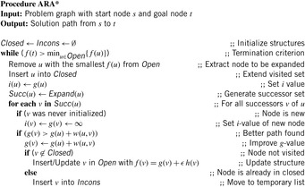
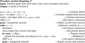
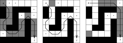
Figure 6.7 shows the operation of ARA* in a simple maze example. Nodes that are inconsistent at the end of an iteration are shown with an asterisk. Although the first call (ϵ = 2.5) is identical to the weighted A* call with the same ϵ, the second call (ϵ = 1.5) expands only one cell. This is in contrast to large number cells expanded by A* search with the same ϵ. For both searches the suboptimality factor, ϵ, decreases from 2.5 to 1.5. Finally, the third call with ϵ set to 1 expands only nine cells.
 |
| Figure 6.7 |
ARA* gains efficiency due to the following two properties. First, each search iteration is guaranteed not to expand nodes more than once. Second, it does not expand nodes of which the i-values before a subroutine call function have already been correctly computed by some previous search iteration.
Each solution ARA* publishes comes with a suboptimality equal to ϵ. In addition, an often tighter suboptimality bound can be computed as the ratio between g(t), which gives an upper bound on the cost of an optimal solution, and the minimum unweighted f-value of an inconsistent node, which gives a lower bound on the cost of an optimal solution. This is a valid suboptimality bound as long as the ratio is larger than or equal to one. Otherwise, g(t) is already equal to the cost of an optimal solution. Thus, the actual suboptimality bound, ϵ′, for each solution ARA* publishes can be computed as the minimum between ϵ and this new bound:
(6.2)
The anytime behavior of ARA* strongly relies on the properties of the heuristics they use. In particular, it relies on the assumption that a sufficiently large inflation factor ϵ substantially expedites the search process. Although in many domains this assumption is true, this is not guaranteed. In fact, it is possible to construct pathological examples where the best-first nature of searching with a large ϵ can result in much longer processing times. In general, the key to obtaining anytime behavior in ARA* is finding heuristics for which the difference between the heuristic values and the true distances these heuristics estimate is a function with only shallow local minima. Note that this is not the same as just the magnitude of the differences between the heuristic values and the true distances. Instead, the difference will have shallow local minima if the heuristic function has a shape similar to the shape of the true distance function. For example, in the case of robot navigation a local minimum can be a U-shaped obstacle placed on the straight line connecting a robot to its goal (assuming the heuristic function is Euclidean distance). The size of the obstacle determines how many nodes weighted A*, and consequently ARA*, will have to visit before getting out of the minimum. The conclusion is that with ARA*, the task of developing an anytime planner for various hard search domains becomes the problem of designing a heuristic function that results in shallow local minima. In many cases (although certainly not always) the design of such a heuristic function can be a much simpler task than the task of designing a whole new anytime search algorithm for solving the problem at hand.
6.2.5. k-Best-First Search
A very different nonoptimal search strategy modifies the selection condition in the priority-queue data structure by considering larger sets of nodes without destroying its internal f-order. The algorithm k-best-first search is a generalization of best-first search in that each cycle expands the best k-nodes from Open instead of the first best node only. Successors are not examined until the rest of the previous k-best nodes are expanded. A pseudo-code implementation is provided in Algorithm 6.17.
In light of this algorithm, best-first search can be regarded as 1-best-first search, and breadth-first search as ∞-best first search, since in each expansion cycle, all nodes in Open are expanded.
The rationale of the algorithm is that if the level of impreciseness in a nonadmissible heuristic function increases, k-best-first search avoids running in the wrong direction and temporarily abandoning overestimated, optimal solution paths. It has been shown to outperform best-first search in a number of domains.
On the other hand, it will not be advantageous in conjunction with admissible, monotonic heuristics, since in this case all nodes that have a cost less than the optimal solution must be expanded anyway. However, when suboptimal solutions are affordable, k-best-first search can be a simple yet sufficiently powerful choice. From this point of view, k-best-first search is a natural competitor not for A*, but for weighted A* with l > 0.5.
6.2.6. Beam Search
A variation of k-best-first search is k-beam search (see Algorithm 6.18). The former keeps all nodes in the Open list, and the latter discards all but the best k nodes before each expansion step. The parameter k is also known as the beam width and can scale close to the limits of main memory. Different from k-best-first search, beam search makes local decisions and does not move to another part of the search tree.
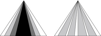
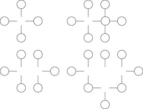
Restricted to blind breadth-first search exploration, only the most promising nodes at each level of the problem graph are selected for further branching with the other nodes pruned off permanently. This pruning rule is inadmissible; that is, it does not preserve the optimality of the search algorithm. The main motivation to sacrifice optimality and to restrict the beam width is the limit of main memory. By varying the beam width, it is possible to change the search behavior; with width 1 it corresponds to a greedy search behavior, with no limits on width to a complete search using A*. By bounding the width, the complexity of the search becomes linear in the depth of the search instead of exponential. More precisely, the time and memory complexity of beam search is O(kd), where d is the depth of the search tree. Iterative broadening (a.k.a. iterative weakening) performs a sequence of beam searches in which a weaker pruning rule is used in each iteration. This strategy is iterated until a solution of sufficient quality has been obtained, and is illustrated in Figure 6.8 (left).
6.2.7. Partial A* and Partial IDA*
During the study of partial hash functions such as bit-state hashing, double bit-state hashing, and hash compact (see Ch. 3), we have seen that the sizes of the hash tables can be decreased considerably. This is paid for by giving up search optimality, since some states can no longer be disambiguated. As we have seen, partial hashing is a compromise to the space requirements that full state storage algorithms have and can be casted as a nonadmissible simplification to traditional heuristic search algorithms. In the extreme case, partial search algorithms are not even complete, since they can miss an existing goal state due to wrong pruning. The probability can be reduced either by enlarging the number of bits in the remaining vector or by reinvoking the algorithm with different hash functions (see Fig. 6.8, right).
Partial A* applies bit-state hashing for A*'s Closed list. The hash table degenerates to a bit array without any collision strategy (we write Closed[i] to highlight the difference). Note that partial A* is applied without reopening, even if the estimate is not admissible, since the resulting algorithm cannot guarantee optimal solutions anyway. The effect of partial state storage is illustrated in Figure 6.9. If only parts of states are stored, more states fit into main memory.
 |
| Figure 6.9 |
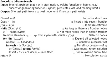
To analyze the consequences of applying nonreversible compression methods, we concentrate on bit-state hashing. Our focus on this technique is also motivated by the fact that bit-state hashing compresses states drastically down to one or a few bits emphasizing the advantages of depth-first search algorithms. Algorithm 6.19 depicts the A* search algorithm with (single) bit-state hashing.
Given M bits of memory, single bit-state hashing is able to store M states. This saves memory of factor  , since the space requirements for an explicit state are at least lg|S| bits. For large state spaces and less efficient state encodings the gains in state space coverage for bit-state hashing are considerable.
First of all, states in the search frontier can hardly be compressed. Second, it is often necessary to keep track of the path that leads to each state. An additional observation is that many heuristic functions and algorithms must access the length (or cost) of the optimal path through which the state was reached.
There are two solutions to these problems: either information is recomputed by traversing the path that leads to the state, or it is stored together with the state. The first so-called state reconstruction method increases time complexity, and the second one increases the memory requirements. Still, state reconstruction needs to store a predecessor link, which on a W-bit processor typically requires W bits.
It is not trivial to analyze the amount of information needed to store the set Open, especially considering that problem graphs are not regular. However, experimental results show that the search frontier frequently grows exponentially with the search depth, such that compressing the set of closed states does not help much. Hence, applying bit-state hashing for search algorithms such as BFS is not as effective as it is in DFS.
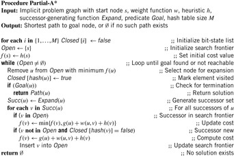
Nonadmissible bit-state hashing can also be used in combination with linear IDA* search. The implementation of Partial IDA* is shown in Algorithm 6.20. Bit-state hashing can be combined with transposition table updates propagating f-values or h-values back to the root, but as the pruning technique is incomplete and annotating any information at a partially stored state is memory intensive, it is simpler to initialize the hash table in each iteration.
Refreshing large bitvector tables is fast in practice, but for shallow searches with a small number of expanded nodes this scheme can be improved by invoking ordinary IDA* with transposition table updates for smaller thresholds and by applying bitvector exploration in large depths only.
6.3. Reduction of the Closed List
When searching tree-structured state spaces, the Closed list is usually much smaller than the Open list, since the number of generated nodes is exponentially growing with search depth. However, in some problem domains its size might actually dominate the overall memory requirements. For example, in the Gridworld problem, the Closed list is roughly described as an area of quadratic size, and the Open list of linear size. We will see that search algorithms can be modified such that, when running out of space during the search, much or all of the Closed list can be temporarily discarded and only later be partially reconstructed to obtain the solution path.
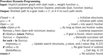
6.3.1. Dynamic Programming in Implicit Graphs
The main precondition of most dynamic programming algorithms is that the search graph has to be acyclic. This ensures a topological order ≼ on the nodes such that u ≼ v whenever u is an ancestor of v.
For example, this is the case for the rectangular lattice of the Multiple Sequence Alignment problem. Typically, the algorithm is described as explicitly filling out the cells of a fixed-size, preallocated matrix. However, we can equivalently transfer the representation to implicitly defined graphs in a straightforward way by modifying Dijkstra's algorithm to use the level of a node as the heap key instead of its g-value. This might save us space, in case we can prune the computation to only a part of the grid. A topological sorting can be partitioned into levels leveli by forming disjoint, exhaustive, and contiguous subsequences of the node ordering. Alignments can be computed by proceeding in rows, columns, antidiagonals, and many more possible partitions.
When dynamic programming traverses a k-dimensional lattice in antidiagonals, the Open list consists of at most k levels (e.g., for k = 2, the parents to the left and top of a cell u at level are at level − 1, and the diagonal parent to the top-left at level − 2); thus, it is of order O(kNk − 1), one dimension smaller than the search space O(Nk).
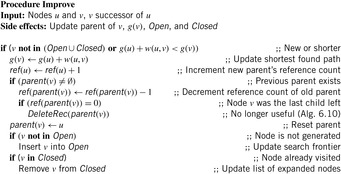
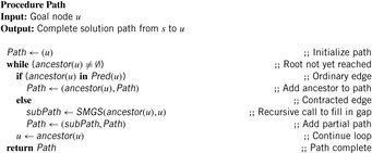
The only reason to store the Closed list is for tracing back the solution path once the target has been reached. A means to reduce the number of nodes that have to be stored for path reconstruction is to associate, similar as in Section 6.1.4, a reference count with each node that maintains the number of children on the optimal path it lies. The pseudo code is shown in Algorithm 6.21 and the corresponding node relaxation step in Algorithm 6.22, where procedure DeleteRec is the same as in Algorithm 6.10.
In general, reference counting has been experimentally shown to be able to drastically reduce the size of the stored Closed list.
6.3.2. Divide-and-Conquer Solution Reconstruction
Hirschberg first noticed that when we are only interested in determining the cost of an optimal alignment, it is not necessary to store the whole matrix; instead, when proceeding by rows, for example, it suffices to keep track of only k of them at a time, deleting each row as soon as the next one is completed. This reduces the space requirement by one dimension, from O(Nk) to O(kNk − 1); a considerable improvement for long sequences. Unfortunately, this method doesn't provide us with the actual solution path. To recover it after termination of the search, recomputation of the lost cell values is needed. The solution is to apply the algorithm twice to half the grid each, once in a forward direction and once in a backward direction, meeting at some intermediate relay layer. By adding the corresponding forward and backward distances, the cell lying on an optimal path can be recovered. This cell essentially splits the problem into two smaller subproblems, one starting at the top-left corner and the other at the bottom-right corner they can be recursively solved using the same method. Since in two dimensions, solving a problem of half the dimension is roughly four times easier, the overall computation time is at most double of that when storing the full Closed list; the overhead reduces even more in higher dimensions. Further refinements of Hirschberg's algorithm exploit additionally available memory to store more than one node on an optimal path, thereby reducing the number of recomputations.
6.3.3. Frontier Search
Frontier search is motivated by the attempt of generalizing the space reduction for the Closed list achieved by Hirschberg's algorithm to a general best-first search. It mainly applies to problem graphs that are undirected or acyclic but has been extended to more general graph classes. It is especially effective if the ratio of Closed to Open list sizes is large. Figure 6.10 illustrates a frontier search in an undirected Gridworld. All generated nodes as well as tags for the used incoming operators prevent reentering the set of expanded nodes, which initially consists of the start state.
 |
| Figure 6.10 |
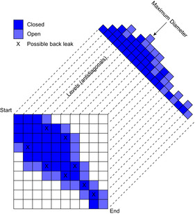
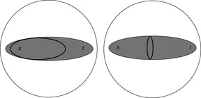
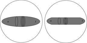
In directed acyclic graphs a frontier search is even more apparent. Figure 6.11 schematically depicts a snapshot during a two-dimensional alignment problem, where all nodes with an f-value no larger than the current fmin have been expanded. Since the accuracy of the heuristic decreases with the distance to the goal, the typical onion-shaped distribution results, with the bulk being located closer to the start node, and tapering out toward higher levels.
However, in contrast to the Hirschberg algorithm, A* still stores all the explored nodes in the Closed list. As a remedy, we obtain two new algorithms.
Divide-and-conquer bidirectional search performs a bidirectional breadth-first search with Closed lists omitted. When the two search frontiers meet, an optimal path has been found, as well as a node on it in the intersection of the search frontiers. At this point, the algorithm is recursively called for the two subproblems: one from the start node to the middle node, and the other from the middle node to the target.
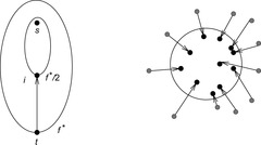
Divide-and-conquer forward frontier search searches only in a forward direction, without the Closed list. In the first phase, a goal t with optimal cost f* is searched. In the second phase the search is reinvoked with a relay layer at about f*/2. When a node on a relay layer is encountered, all its children store it as their parent. Subsequently, every node past the relay layer saves its respective ancestor on the relay layer that lies on its shortest path from the start node. When the search terminates, the stored node in the relay layer is an intermediate node roughly halfway on an optimal solution path. This intermediate state i from s to t is detected; in the last phase the algorithm is recursively called for the two subproblems from s to i, and from i to t. Figure 6.12 depicts the recursion step (left) and the problem in directed graphs of falling back behind the current search frontier (right), if the width of the search frontier is too small. For this case, several duplicates are generated.
 |
| Figure 6.12 |
Apart from keeping track of the solution path, A* uses the stored Closed list to prevent the search from leaking back, in the following sense. A consistent heuristic ensures that (as in the case of Dijkstra's algorithm) at the time a node is expanded, its g-value is optimal, and hence it is never expanded again. However, if we try to delete the Closed nodes, then there can be topologically smaller nodes in Open with a higher f-value; when those are expanded at a later stage, they can lead to the regeneration of the node at a nonoptimal g-value, since the first instantiation is no longer available for duplicate checking. In Figure 6.11, nodes that might be subject to spurious reexpansion are marked “X.” The problem of the search frontier “leaking back” into previously expanded Closed nodes is the main obstacle for Closed list reduction in a best-first search.
One suggested workaround is to save, with each state, a list of move operators describing forbidden moves leading to Closed nodes. However, this implies that the node representation cannot be constant, but grows exponentially with the problem dimension. Another way out is to insert all possible parents of an expanded node into Open specially marked as not yet reached. However, this inflates the Open list and is incompatible with many other pruning schemes.
6.3.4. *Sparse Memory Graph Search
The reduction of frontier search has inspired most of the upcoming algorithms. A promising attempt at memory reduction is sparse memory graph search (SMGS). It is based on a compressed representation of the Closed list that allows the removal of many, but not all, nodes. Compared to frontier search it describes an alternative scheme of dealing with back leaks.
Let Pred(v) denote the set of predecessors for node v; that is,  . The kernel K(Closed) of the set of visited nodes Closed is defined as the set of nodes for which all predecessors are already contained in Closed:
 The rest of the Closed nodes are called the boundary B(Closed):
The Closed nodes form a volume in the search space enclosing the start node; nodes outside this volume cannot reach any node inside it without passing through the boundary. Thus, storing the boundary is sufficient to avoid back leaks.
A sparse solution path is an ordered list  with d ≥ 1 and
  ; that is, it consists of a sequence of ancestor nodes on an optimal path where vi doesn't necessarily have to be a direct parent of vi + 1. All Closed nodes except boundary nodes and relay nodes can be deleted, such as nodes that are used to reconstruct the corresponding solution path from the sparse representation. SMGS tries to make maximum use of available memory by lazily deleting nodes only if necessary because the algorithm's memory consumption approaches the computer's limit.
The algorithm SMGS assumes that the in-degree |Pred(v)| of each node v can be computed. Moreover, the heuristic h must be consistent,  for edge u, v, so that no reopening can take place. SMGS is very similar to the standard algorithm, except for the reconstruction of the solution path, which is shown in Algorithm 6.23. Starting from a goal node, we follow the ancestor pointers as usual. However, if we encounter a gap, the problem is dealt with a recursive call of the search procedure. Two successive nodes on the sparse path are taken as start and goal node. Note that these decomposed problems are by far smaller and easier to solve than the original one.
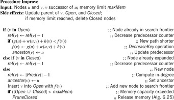
Algorithm 6.24 illustrates the edge relaxation step for SMGS. Each generated and stored node u keeps track of the number of unexpanded predecessors in a variable ref(u). It is initialized with the in-degree of the node minus one, accounting for its parent. During expansion the ref-value is appropriately decremented; kernel nodes can then be easily recognized by ref(u) = 0.
The pruning procedure (see Alg. 6.25) prunes nodes in two steps. Before deleting kernel nodes, it updates the ancestral pointer of its boundary successors to the next higher boundary node. Further pruning of the resulting relay nodes is prevented by setting its ref-value to infinity.
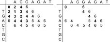
Figure 6.13 gives a small example for the algorithm in the context of the multiple sequence alignment problem. The input consists of the two strings TGACTGC and ACGAGAT, assuming that a match incurs no cost, a mismatch introduces cost 1, and a gap corresponds to cost 2.
 |
| Figure 6.13 |

6.3.5. Breadth-First Heuristic Search
The term breadth-first heuristic search is short for the sparse-memory algorithm breadth-first branch-and-bound search with layered duplicate detection. It is based on the observation that the storage of nodes serves two purposes. First, duplicate detection allows recognition of states that are reached along a different path. Second, it allows reconstruction of the solution path after finding the goal using the links to the predecessors. IDA* can be seen as a method that gives up duplicate detection, and breadth-first heuristic search gives up solution reconstruction.
Breadth-first search divides the problem graph into layers of increasing depth. If the graph is unit cost, then all nodes in one layer have the same g-value. Moreover, as shown for frontier search at least for regular graphs, we can omit the Closed list and reconstruct the solution path based on an existing relay layer kept in main memory.
Subsequently, breadth-first heuristic search combines breadth-first search with an upper-bound pruning scheme (that allows the pruning of frontier nodes according to the combined cost function f = g + h) together with frontier search to eliminate already expanded nodes. The assumption is that the sizes of the search frontiers for breadth-first and best-first search differ and that using divide-and-conquer solution reconstruction is more memory efficient for breadth-first search.
Instead of maintaining used operator edges together with each problem graph node, the algorithms maintain a set of layers of parent nodes. In undirected graphs two parent layers are sufficient, as the successor of a node that is a duplicate has to appear either in the actual layer or in the layer of previous nodes. More formally, assume that the levels Open0, …, Openi − 1 have already been computed correctly. We consider a successor v of a node u ∈ Openi − 1: The distance from s to v is at least i − 2 because otherwise the distance of u would be less than i − 1. Thus,  . Therefore, we can correctly subtract Openi − 1 and Openi − 2 from the set of all successors of Openi − 1 to build the duplicate-free search frontier Openi for the next layer.
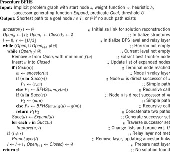
Suppose that an upper bound U on the optimal solution cost f* is known. Then node expansion can immediately discard successor nodes of which the f-values are larger than U. The pseudo-code implementation using two backup BFS layers for storing states assumes an undirected graph and is shown in Algorithm 6.26 and Algorithm 6.27. The lists Open and Closed are partitioned along the nodes' depth values. The relay layer r is initially set to  . During the processing of layer l the elements are moved from Openl to Closedl and new elements are inserted into Openl + 1. After a level is completed l increases. The Closed list for layer l and the Open list for layer (l + 1) are initialized to the empty set. In case a solution is found the algorithm is invoked recursively to enable divide-and-conquer solution reconstruction from s to m and from m to the established goal u, where m is the node in relay layer r that realizes minimum costs with regard to u. Node m is found using the link ancestor(u), which in case a previous layer is deleted, is updated as follows. For all nodes u below the relay layer we set ancestor(u) to s. For all nodes above the relay layer we set ancestor(u) to ancestor(ancestor(u)) unless we encounter a node in the relay layer. (The implementation of DeleteLayer is left as an exercise.)
If all nodes were stored in the main memory, breadth-first heuristic search would usually traverse more nodes than A*. However, like sparse memory graph search, the main impact of breadth-first heuristic search lies in its combination with divide-and-conquer solution reconstruction. We have already encountered the main obstacle for this technique in heuristic search algorithms—the problem of back leaks; to avoid node regeneration, a boundary between the frontier and the interior of the explicitly generated search graph has to be maintained, which dominates the algorithm's space requirements. The crucial observation is that this boundary can be expected to be much smaller for breadth-first search than for best-first search; an illustration is given in Figure 6.14. Essentially, a fixed number of layers suffices to isolate the earlier layers. In addition, the implementation is easier.
 |
| Figure 6.14 |
As said, BFHS assumes an upper bound U on the optimal solution cost f* as an input. There are different strategies to find U. One option is to use approximate algorithms like hill-climbing or weighted A* search. Alternatively, we can use an iterative-deepening approach as in IDA*, starting with U ← h(s) and continuously increasing the bound. Since the underlying search strategy is BFS, the algorithm has been called breadth-first iterative deepening.
 |
| Algorithm 6.27. |
| Update of a problem graph edge in Algorithm 6.26. |
6.3.6. Locality
How many layers are sufficient for full duplicate detection in general is dependent on a property of the search graph called locality.
Definition 6.2
(Locality) For a weighted problem graph G the locality is defined as
For undirected and unweighted graphs we have w ≡ 1. Moreover, δ(s, u) and δ(s, v) differ by at most 1, so that the locality turns out to be 2. The locality determines the thickness of the search frontier needed to prevent duplicates in the search. Note that the layer that is currently expanded is included in the computation of the locality but the layer that is currently generated is not.
While the locality is dependent on the graph, the duplicate detection scope also depends on the search algorithm applied. We call a search graph a g-ordered best-first search graph if each node is maintained in buckets matching its g-value. For breadth-first search, the search tree is generated with increasing path lengths, whereas for weighted graphs the search tree is generated with increasing path cost (this corresponds to Dijkstra's exploration strategy in 1-Level Bucket data structure).
Theorem 6.2
(Locality Determines Boundary) The number of buckets of a g-ordered best-first search graph that need to be retained to prevent a duplicate search effort is equal to the locality of the search graph.
Proof
Let us consider two nodes u and v, with v ∈ Succ(u). Assume that u has been expanded for the first time, generating the successor v, which has already appeared in the layers  , implying
  . We have
 This is a contradiction to w(u, v) > 0.
To determine the number of shortest path layers prior to the search, it is important to establish sufficient criteria for the locality of a search graph. However, the condition  maximized over all nodes u and v ∈ Succ(u) is not a property that can be easily checked before the search. So the question is, can we find a sufficient condition or upper bound for it? The following theorem proves the existence of such a bound.
Theorem 6.3
(Upper Bound on Locality) The locality of a problem graph can be bounded by the minimal distance to get back from a successor node v to u, maximized over all u, plus w(u, v).
Proof
For any nodes s, u, v in a graph, the triangular property of shortest paths  is satisfied, in particular for v ∈ Succ(u). Therefore,
  and
and 
 . In positively weighted graphs, we have
  , such that
  is larger than the locality.
Theorem 6.4
(Upper Bounds in Weighted Graphs) For undirected graphs with maximum edge weight C we have localityG ≤ 2C.
Proof
For undirected graphs with with maximum edge cost C we have
6.4. Reduction of the Open List
In this section we analyze different strategies that reduce the number of nodes in the search frontier. First we look at different traversal policies that can be combined with a branch-and-bound algorithm.
Even if the number of stored layers k is less than the locality of the graph, the number of times a node can be reopened in breadth-first heuristic search is only linear in the depth of the search. This contrasts the exponential number of possible reopenings for linear-space depth-first search strategies.
6.4.1. Beam-Stack Search
We have seen that beam search accelerates a search by not maintaining in each layer just one node, but a fixed number, maxMem. No layer of the search graph is allowed to grow larger than the beam width so that the least-promising nodes are pruned from a layer when the memory is full. Unfortunately, this inadmissible pruning scheme means that the algorithm is not guaranteed to terminate with an optimal solution.
Beam-stack search is a generalization of beam search that essentially turns it into an admissible algorithm. It first finds the same solution like beam search, but then continues to backtrack to pruned nodes to improve the solution over time. It can also be seen as a modification of branch-and-bound search, and includes depth-first branch-and-bound search and breadth-first branch-and-bound search as special cases. In the first case the beam width is 1, and in the second case, the beam width is greater than or equal to the size of the largest layer.
The first step toward beam-stack search is divide-and-conquer beam search. It limits the layer width of breadth-first heuristic search to the amount of memory available. For undirected search spaces, divide-and-conquer beam search stores three layers for duplicate detection and one relay layer for solution reconstruction. The difference from traditional beam search is that it uses divide-and-conquer solution reconstruction to reduce memory. Divide-and-conquer beam search has been shown to outperform, for example, weighted A* in planning problems. Unfortunately, as with beam search, it is neither complete nor optimal. An illustration of this strategy is provided in Figure 6.15. To the left we see the four layers (including the relay layer) of currently stored breadth-first heuristic search. To the right we see that divide-and-conquer beam search explores a smaller corridor, leading to less nodes to be stored in main memory.
 |
| Figure 6.15 |
The beam-stack search algorithm utilizes a specialized data structure called the beam stack, a generalization of an ordinary stack used in DFS. In addition to the nodes, each layer also contains one record of the breadth-first search graph. To allow backtracking, the beam stack exploits the fact that the nodes can be sorted by their cost function f. We assume that the costs are unique, and that ties are broken by refining the cost function to some secondary order comparison criteria. On the stack in each layer a half-open interval  is stored, such that all nodes u are pruned with
  and all nodes are eliminated with an
  . All layers are initialized to [0, U) with U being the current upper bound.
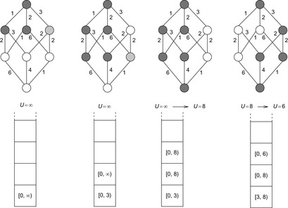
An illustration of beam-stack search is provided in Figure 6.16. The algorithm is invoked with a beam width of 2 and an initial upper bound of ∞. The problem graph is shown at the top of the figure. Nodes currently under consideration are shaded. Light shading corresponds to the fact that a node cannot be stored based on the memory restriction. To the bottom of the graphs, the current value for U and the contents of the beam stack are provided. We have highlighted four iterations. The first iteration expands the start node and generates two of three successors for the next search depth. As all weights are integers, the next possible value 3 is stored as the upper bound for the first layer. When expanding the second layer, again one node does not satisfy the width. In the next iteration we arrive at the goal on two possible paths, suggesting a minimal solution of 8. The value overwrites the initial upper bound and is propagated bottom-up such that 8 is the next upper bound to start with. As we have searched all paths corresponding to a solution value smaller than 3, the lower bound is set to 3. The last step shows the situation for searching the graph with the solution interval [3, 8]. It illustrates that beam-stack search eventually finds the optimal solution of value 6, which in turn is assigned to U and reported at the root node.
 |
| Figure 6.16 |
Divide-and-conquer beam-stack search combines divide-and-conquer solution reconstruction with the beam stack search. If the memory becomes full, the nodes with the highest f-values are deleted from the Open list. In divide-and-conquer beam-stack search there are two complications to be resolved. First, divide-and-conquer solution reconstruction has to be combined with backtracking. Since there are only a bounded number of layers in memory, the layer to which the algorithm backtracks may not be in memory, so that it has to be recovered. Fortunately, the beam-stack search contains the interval of f-values to recover a missing layer. The algorithm goes back to the start node and generates successor nodes at each layer according to the corresponding beam-stack item, until all nodes in the layer preceding the missing layer have been expanded. The other problem is the decision on solution reconstruction or continuation of the search. If the algorithm starts reconstructing the solution path using large amounts of memory, then the search information computed so far is affected. For these cases a delayed solution reconstruction approach is useful. Solution construction starts only if the search algorithm backtracks, since this will delete search layers anyway.
Algorithm 6.28 shows a recursive pseudo-code implementation of the search algorithm. Initially, the entire interval [0, U] is pushed onto the beam stack. As long as no solution is found, which means that there are unexplored intervals on the beam stack, a recursive search procedure beam-stack-search works on one interval from the initial node. If a solution is found, then the upper-bound value is updated. Subsequently, the refined upper-bound value truncates and eliminates the intervals on the beam stack. A goal has been found if the upper-bound is exceeded, otherwise the interval can be shortened by the explored part.
To arrive at linear space performance of O(d ⋅ maxMem) elements, procedure PruneLayer restricts the number of nodes stored. When beam-stack search prunes nodes in a layer, it changes the fmax of the previous layer's stack item to the lowest costs of the nodes that have been pruned. This ensures that the search algorithm will not generate any successor with a larger f-cost before backtracking to this layer. Backtracking is invoked if all successors of nodes in the current layer have a w-value greater than U. On every backtrack, beam-stack search forces the search beam to admit a different set of successors by shifting the interval  ; that is, the new fmin-value is initialized with fmax and fmax is initialized with U.
Theorem 6.5
(Optimality of Beam-Stack Search) Beam-stack search is guaranteed to find an optimal solution.
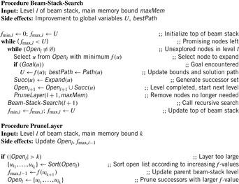
Proof
We first show that beam-stack search always terminates. If Δ > 0 is the least operator cost then the maximum length of a path and the maximum depth of the beam stack is at most  . If b is the maximal number of applicable operators (a.k.a. the maximal out-degree of the problem graph), the number of backtracks in beam stack search is bounded by
  .
.
Moreover, beam-stack search systematically enumerates all successors of a level by shifting the interval  of path costs. Therefore, no path will be ignored forever, unless the beam stack contains a node u with f(pu) > U or a node to which a lower-cost path has already been found. Thus, an optimal path must be found eventually.
As beam-stack search is a generalization to the two other branch-and-bound algorithms mentioned earlier, with this proof we have also shown their optimality.
An illustration of divide-and-conquer beam-stack search is provided in Figure 6.17 (right). Different from ordinary beam-stack search (left), intermediate layers are eliminated from main memory. If a solution has been found, it has to be reconstructed. The beam width is induced by the resources of main memory.
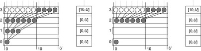
6.4.2. Partial Expansion A*
The main observation that led to the development of Partial Expansion A* (PEA*) is that classic A* search expands a node by always generating all of its successors. However, many of these nodes have an f-value larger than the optimal solution and hence will never be selected. They just clutter the Open list and waste space.
In PEA* (see Algorithm 6.29 and Algorithm 6.30), each node stores an additional value F, which is the minimum f-value of all of its yet nongenerated children. In each iteration, only a node in Succ≤ with the minimum F-value is expanded, and only those children with f = F can be inserted into Open. After expansion, a node is moved to the Closed list, only if it has no more nongenerated successors left; otherwise, its F-value is updated to reflect the possible increase in f-value due to the shrinking of set Succ>.
This algorithm has the advantage of only generating nodes with an f-value smaller than the optimal cost, which cannot be avoided altogether. In experimental results in the domain of Multiple Sequence Alignment, it has been shown to be able to reduce the space memory requirement by about a factor of a hundred. However, the overhead in computation time can be considerable, since for minimum determination all possible edges have to be considered, while only a few of them will actually be retained. As a remedy, it was proposed to relax the condition by generating all children with f ≤ F + c at once, for some small constant c.
Figure 6.18 illustrates an example for PEA*. We see the first four expansion steps. In the first expansion the f-value of the root is initialized to 1. Only one child node is stored at this expansion, because the f-value of it equals the f-value of the root. The root's f-value is revised to 2, and it is reinserted into Open. In the second expansion there are no successors with the same f-value as the expanded node, so nothing is stored during this expansion. The expanded node is reinserted into Open after revising its f-value 3. In the third expansion the root is expanded again and the second successor is stored. The root's f-value is revised to 4, and again inserted into Open.
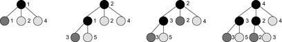 |
| Figure 6.18 |
Note the similarity of the underlying idea to that of algorithm RBFS (see Sec. 5.8, p. 219), which also prunes the search tree below a node if the f-values start to exceed that of a sibling.
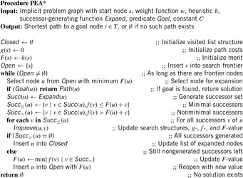
6.4.3. Two-Bit Breadth-First Search
Two-bit breadth-first search integrates a tight compression method into the BFS algorithm. The approach designed for solving the large search problems requires a reversible minimum perfect hash functions to be available. It applies a space-efficient representation for a bitvector state space representation in breadth-first search with two bits per state.
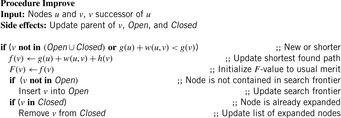
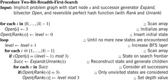
Algorithm 6.31 shows how to generate the state spaces according to such a bitvector. The running time is (roughly) determined by the size of the search space times the maximum BFS layer (times the efforts to generate the children).
The algorithm uses two bits encoding the numbers from 0 to 3, with 3 denoting an unvisited state, and 0, 1, and 2 denoting the mod-3 value of the current depth. The main effect is to distinguish newly generated states and already visited states from the current layer that is scanned. If a bit is set to be expanded the array index is unranked and the successors are produced. The successor state bits are computed using a rank function and then marked with the mod-3 value of their depth.
In the advent of a move-alternation property that lets us distinguish states in one BFS level from the previous ones we can perform bitvector BFS using only one bit per state. For the example of such property changes with each depth, consider the (n2 − 1)-Puzzle with an even number of columns. The position of the blank can be used to derive the parity of the BFS layer (the blank position in puzzles with an odd number of columns at an even BFS level is even and for each odd BFS level it is odd).
Two-bit breadth-first search suggests the use of bitvectors to compress pattern databases to lg 3 ≈ 1.6 bits per abstract state (value 3 for an unvisited state is obsolete). If we stored the mod-3 value of the BFS level in a hash table, we can determine its absolute value by backward construction incrementally as one shortest path predecessor with a mod-3 value of BFS-level k contained in level k − 1 mod 3.
6.5. Summary
We have seen a sizable number of attempts to tame the explosion of the state space working at the limit of main memory. Exploiting various hybrids of A* and IDA* exploration has given rise to different trade-offs between the time of regenerating a node and the space for storing it to detect duplicates. The presented techniques provide a portfolio for tackling a challenging state space exploration problem at the edge of main memory, provided that no better guidance is known.
There are three sources of inefficiency of IDA* that have been addressed. First, in a graph where we have multiple paths to a node, IDA* repeats work due to the large number of duplicates. Second, each IDA* iteration repeats all the work of the previous iteration. This is necessary because IDA* uses essentially no storage. IDA* uses a left-to-right traversal of the search frontier. If thresholds are increased too rapidly, then IDA* may expand more nodes than necessary. In contrast, A* maintains the frontier in sorted order, expanding nodes in a best-first manner, which incurs some cost for handling the data structures.
The repeated states problems have been solved using a transposition table as a cache of visited states. The table is usually implemented as a large hash dictionary to minimize the lookup costs. A transposition table entry essentially stores and updated h-values. It serves two purposes and its information can be split in the minimal g-value for this state and the backed-up f-value obtained from searching this state. The g-values are used to eliminate provably nonoptimal paths from the search. The f-values are used to show that additional search at the node for the current iteration threshold is unnecessary. For larger state vectors a better coverage of the search space has been achieved by applying inadmissible compaction methods like bit-state hashing.
If heuristics are rather weak, their influence can be scaled in weighted heuristic search variants like weighted A* using node priorities  . In some cases, the loss of solution quality can be bounded to obtain ϵ-optimal solutions. Another completeness preserving strategy, appropriate especially for inconsistent heuristics, is k-best-first search, which selects the k-best nodes from the priority queue. Its aggressive variant, k-beam search, removing all other nodes from the queue, is often faster but incomplete.
ITS aims to span the gap between A* and IDA* by using whatever memory is available to reduce the duplicated node generations that make IDA* inefficient. SMA* chooses for expansion the deepest, least f-cost node. ITS exploration order, by contrast, is left-to-right depth-first. New nodes are inserted into a data structure representing the search tree, and the node chosen for expansion is the deepest, left-most node of which the f-value does not exceed the current cost bound. ITS requires the whole tree structure to retract nodes if it runs out of memory. Fringe search also explores successors from left to right but with a simpler data structure.
The advantage of state-caching algorithms is that they explore the middle ground between time and space of IDA* and A* searches. The disadvantages of many state-caching algorithms is that their successes in practice are rather small. State-caching distinguishes between the virtual search tree that has been traversed so far and the part of it that resides in main memory. The main challenge is to dynamically change the set of stored nodes according to the (possibly asymmetrically) growing search tree, without losing efficiency gains for node expansion. We observe a trade-off between the depth of the search and its width, or, more generally speaking, between exploration and exploitation of the search space.
Another set of memory-restricted algorithms, including frontier search, breadth-first heuristic search, sparse-memory graph search, and beam-stack search, eliminate already expanded nodes from the memory while preventing the algorithms to take a back-edge to fall behind the search frontier. The largest of such back-edges defines the locality and is, therefore, dictated by the structure of the problem graph. In undirected graphs, only three BFS layers need to be stored in the RAM, while in acyclic graphs, only one layer is needed.
Some of the algorithms, like breadth-first heuristic search, sparse-memory graph search, and beam-stack search, additionally stress the fact that for a limited duplicate detection, scope, breadth-first search together with an upper bound on the solution cost saves more memory. The problem of reconstructing the solution path is considered using divide-and-conquer based on information stored in relay layers.
For reducing the search frontier, we have looked at partial expansion algorithms, which expand nodes but but only store one successor. Such algorithms show a benefit in case the search frontier grows exponentially.
Moreover, we have shown that provided a perfect and reversible hash function, two bits are sufficient to conduct a complete breadth-first exploration of the search space.
Table 6.3 summarizes the presented approaches to memory-restricted search. We give information on the algorithm's implementation and whether to save space it mainly reduces the Open or the Closed list. We also give information if the space limit is on the number of states or bits or if it is logarithmic in the state space size. We provide information on possible edge weights in the problem graph. For constant-depth solution reconstruction implementations, undirected graphs are assumed. Most of the algorithms can be extended to weighted and directed problem graphs. However, including these extensions can be involved. Last but not least, the table shows whether or not the algorithm is optimal when assuming admissible heuristic estimates.
For an exploration at the edge of the main memory, it is obvious that due to time overhead for swapping of memory pages, saving memory eventually saves time.
6.6. Exercises
6.1 Consider depth-first search (with duplicate detection) that continues the exploration when a goal has been found and that bounds the search to the depth of that state minus 1. Initially, there is a depth bound that is set to a certain upper-bound value by the user.
1. Show that the strategy can also be trapped by the anomaly described in the text.
2. Given an example of an unweighted problem graph with not more than six nodes, where does the anomaly arise? How large is your depth bound?
3. Fix the problem to make the algorithm admissible.
6.2 Figure 6.19 provides an example for the effect of SNC. On the left it shows that IDA* with a transposition table caches nodes a, b, d in the order of expansion. In contrast, SNC is likely to store node e that is visited more often. As e is detected as a duplicate state, the entire subtree below e (not shown) is not repeatedly explored.
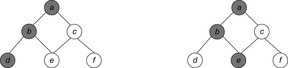
1. Generate a random 100 maze and plot the probability of caching nodes p = 0, p = 0.2, p = 0.4, p = 0.6, p = 0.8, and p = 1 with respect to the number of times the same node is expanded.
2. To which algorithm does SNC reduce for p = 0 and p = 1?
6.3 In Extended IDA* (see Alg. 6.32) states are expanded in A*-like fashion with the exception that the maximum cost value in the priority queue is not exceeded. The first stage collects at most m states in running memory-bounded IDA*. The queue additionally allows access to the element of maximal cost. In the second stage of the algorithm the collected frontier nodes in D are selected and expanded. Successor nodes v of u are reinserted into D if they are safe (i.e., if D is not full and the f-value of v is smaller than the maximal f-value in the priority queue). This is done until D eventually becomes empty. The very last expanded node in the second phase then gives the bound for the next IDA* exploration. Show that
1. All x in D have not been expanded.
2. For each x in D we have  and
and  of all generated but not expanded nodes u.
3. For all expanded nodes u we have  , and if
  then u has been expanded.
4. The algorithm terminates with an optimal solution.
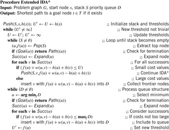
6.4 In enforced hill-climbing search give plausible definitions for
1. A harmless, a recognized, and an unrecognized dead-end.
2. A local minima and a (maximal) exit distance.
6.6 Let us investigate the notion of node inconsistency:
1. Suppose that every node in the state space is consistent. Show that a solution path from s to t is then an optimal one in the graph.
2. Suppose that no node in the state space is underconsistent. Can you say anything about the relationship between the cost of a solution path from s to t and g(t)? If yes, then prove the relationship.
3. Suppose that every underconsistent node s in the state space has v(s) + h(s) > g(t). Can you then say anything about the relationship between the cost of a solution path from s to t and g(t)? If yes, then prove the relationship.
6.7 Anytime A* continues to expand nodes after the first solution is found according to the same priority function, prune away from Open the nodes with unweighted f-values (g(u) + h(u), where h(u) is uninflated) larger than the cost of the best solution found so far, g(t).
Analyze the amount of work (in terms of nodes expanded) that anytime algorithms have to do to generate their first solutions. Assume that all algorithms have the same tie-breaking criteria when choosing between two nodes with the same priorities for expansion.
1. Given the same consistent heuristics, is it possible for ARA* to do more work than (uninflated) A* before generating a first solution? Prove the answer.
2. Given the same consistent heuristics and the same initial ϵ, is it possible for ARA* to do more work than anytime A* before generating a first solution? Prove the answer.
3. Given the same consistent heuristics and the same initial ϵ, is it possible for anytime A* to have more nodes in Open than for ARA* at the time each algorithm generates a first solution? What about the other way around? Prove your answers.
6.8 Compare k-best-first search with weighted A* and beam search on a randomly generated graph of 15 nodes with a consistent heuristic and a nonadmissible heuristic. To generate the graph, throw a biased coin with probability of 20% for drawing an edge between a pair of vertices.
6.9 Figure 6.20 shows a typical tree in SMAG, where the left subtree has been pruned to make room for the more promising right subtree. The f-costs that are propagated bottom-up are shown with their original f-costs. Nodes are generated in the order of their number. The pruned region is shown.
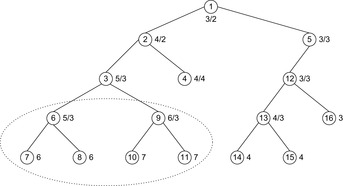
1. In which order are the nodes pruned?
2. Explain how node 9 will receive a value of 5, although it was known to have a value of 6.
6.10 Run frontier breadth-first search in the Gridworld.
1. Compute the exact number of nodes in level i.
2. Determine the accumulated number of nodes in the levels 1, …, i.
3. Quantify the ratio of Open and Closed list sizes for a given level.
4. Determine the ratio of Open and Closed list sizes in the limit for a large BFS level.
6.12 Complete the table in Figure 6.13 for pruning the Multiple Sequence Alignment problem with SMGS.
1. Compute the optimal alignment costs.
2. Invoke one additional memory reduction phase.
3. Reconstruct the solution path.
6.13 Implement procedure PruneLayer for breadth-first heuristic search in pseudo code.
6.14 One problem of beam-stack search are large plateaus of nodes that have the same f-value and that exceed the memory capacity. Discuss beam-stack variants that
1. Solve the problem by refining the comparison operation.
2. Explore such plateaus completely using disk.
3. Enforce a monotone cost function by considering a lexicographic ordering on states.
6.15 A simplification of the two-bit breadth-first search algorithm allows us to generate the entire state space using only one bit. Algorithm 6.33 participates from the implicit ordering imposed by the minimum perfect hash function for the (n2 − 1)-Puzzle (see Ch. 3). As the algorithm does not distinguish between Open and Closed nodes, the algorithm may expand a node multiple times. If the successor's position is smaller than the actual one, it will be expanded in the next run, otherwise in the same one.
1. Show that the number of scans in the algorithm one-bit-reachability is bounded by the maximum BFS layer.
2. Can you avoid multiple node expansions?
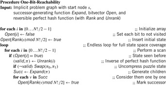
6.7. Bibliographic Notes
Memory-restricted search has been studied from different angles for the last three decades. We only refer to some milestones. There are many others like m-depth search by Ibaraki (1978) and speculative search by Gooley and Wah (1990). The anomaly of depth-bounded DFS has been described in Edelkamp, Leue, and Lluch-Lafuente (2004c). Admissible DFS has been implemented in the model checker SPIN by Holzmann (2004).
One of the first memory-restricted algorithms is the recursive best-first-search algorithm MREC that has been proposed by Sen and Bagchi (1989). The algorithm is a generalization of IDA* that uses additional memory. It grows an explicit search graph until the main memory limit is reached. The memory usage is static and supports no caching strategy. If the pool size is set to 0, then MREC behaves identical to IDA*. Like IDA*, MREC starts all iterations at the root node, so that the underlying problem graph is repeatedly searched. This avoids a priority queue representation of the list of generated nodes.
Transposition tables have been suggested for IDA* exploration by Reinefeld and Marsland (1994) in the context on improved puzzle solving. The term is inherited from two-player game search, where move transpositions are detected by hashing. Avoiding multiple searches from identical nodes, transposition tables speed up the search of the game/search tree considerably. Stochastic node caching is due to Miura and Ishida (1998) and has been successfully applied to multiple sequence alignment problems. Different to our exposition, SNC is presented in the context of the MREC algorithm.
MA* has been introduced by Chakrabarti, Ghose, Acharya, and DeSarkar (1989). Russell (1992) has simplified the exposition and improved it by incorporating the path-max heuristic (SMA*). Kaindl and Khorsand (1994) have generalized it to graph search (SMAG). Zhou and Hansen (2003b) have improved its efficiency when reopening nodes. Iterative threshold search (ITS) has been proposed by Ghosh, Mahanti, and Nau (1994). IDA* with bit-state hashing has first been proposed in the context of protocol validation by Edelkamp, Leue, and Lluch-Lafuente (2004b). It has been brought to AI by Hüffner, Edelkamp, Fernau, and Niedermeier (2001) to optimally solve Atomix instances.
As discussed in the text, earlier approaches in memory-restricted search had only limited success in exploring the middle-ground between A* and IDA*. As one reason, the overhead for implementing the caching policies often did not pay off. Recent algorithms appear more careful in testing applicability. Often acyclic or undirected search spaces are assumed. Algorithm RIDA* has been presented by Wah and Shang (1994). Zhou and Hansen (2003a) have presented the approach to prune the Closed list in A* and Yoshizumi, Miura, and Ishida (2000) introduced Partial Expansion A*. The algorithm of Hirschberg (1975) has influenced Korf (1999) in the development of the divide-and-conquer strategy frontier search for multiple sequence alignment problems. The approach has been improved by Korf and Zhang (2000) into a forward search algorithm. Divide-and-conquer beam search has been presented by Zhou and Hansen (2004a) and its extension to beam-stack search by Zhou and Hansen (2005b).
The time complexity of SMAG has also been established for the algorithm DBIDA*, developed by Eckerle and Schuierer (1995). It dynamically balances the search tree. The algorithm, its bidirectional variant, and a lower-bound example have been studied by Eckerle (1998),. The question of how to add diversity into the search has been posed in the context of a memory-restricted k-breadth-first search algorithm by Linares Lòpez and Borrajo (2010).
The discussion of inadmissable heuristics in weighted A* is kept rather short. Pearl (1985) already dedicated one entire chapter to that subject. In Chapter 2 we saw that the number of reopenings can be exponential. We followed the approach of inadmissible nodes by Likhachev (2005). On top of work by Zahavi, Felner, Schaeffer, and Sturtevant (2007) and by Zhang, Sturtevant, Holte, Schaeffer, and Felner (2009), Thayer and Ruml have studied both an inadmissible heuristic to quickly find a solution and an admissible one to guarantee optimality.
Enforced hill-climbing has been proposed by Hoffmann and Nebel (2001) in the context of action planning. It has been adapted to both propositional and numerical planning by Hoffmann (2003). In case of failure in a directed problem graph the planner chooses best-first search (with f = g + 5h as a default) as complete back-end. In the book by Hoos and Stützle (2004) (on the very first page) the pseudo code of the iterative improvement algorithm is presented. The algorithm shares many similarities with enforced hill-climbing and was known before enforced hill-climbing was introduced.
Adjusting the weights in A* has been studied in detail by Pohl (1977a). The presentation of ϵ-optimal approximation for A* with node selection based on search efforts refers to results presented by Pearl (1985). The algorithm k-best-first search is introduced by Felner (2001) and empirically evaluated in the incremental random trees with dead-ends, in sliding-tile puzzles, and in number partition problems. Although beam search is often associated with a breadth-first strategy, Rich and Knight (1991) have suggested applying it to best-first search. A more general definition has been given by Bisani (1987), where any search algorithm that uses pruning rules to discard nonpromising alternatives is called beam search. One example for the adaption to the depth-first branch-and-bound search algorithm is provided by Zhang (1998). He used iterative weakening, as introduced by Provost (1993), to regain completeness. A closely related technique is iterative broadening by Ginsberg and Harvey (1992). Beam search has been applied to accelerate bug-hunting in model checking by Wijs (1999).
The idea of anytime search was proposed in the AI community a while ago (Dean and Boddy, 1988), and much work has been done on the development of anytime planning algorithms since then (e.g., Ambite and Knoblock, 1997; Hawes, 2002; Pai and Reissell, 1998; Prendinger and Ishizuka, 1998; Zilberstein and Russell, 1993). A* and its variants, such as weighted A*, can easily run out of memory in cases when the heuristics guide the search in a wrong direction and the state space is large. Consequently, these properties extend to the anytime algorithms that are based on weighted A* such as ARA* by Likhachev (2005). Specific memory-bounded anytime heuristic searches, for example, have been developed by Furcy (2004), Kumar (1992), Zhang (1998). The term potential search has been coined by Stern, Puzis, and Felner (2010b) to describe an approach to greedy anytime heurstic search. A framework on anytime heuristic search has been provided by Thayer and Ruml (2010).
An anytime search algorithm is suitable for solving complex planning problems under the conditions where time is critical. An incremental search is suitable for planning in domains that require frequent replanning (e.g., dynamic environments). Search methods for dynamic graph updates have been suggested in the algorithms literature; for example, by Ausiello, Italiano, Marchetti-Spaccamela, and Nanni (1991); Even and Shiloach (1981); Even and Gazit (1985); Edelkamp (1998a); Feuerstein and Marchetti-Spaccamela (1993); Franciosa, Frigioni, and Giaccio (2001); Frigioni, Marchetti-Spaccamela, and Nanni (1996); Goto and Sangiovanni-Vincentelli (1978); Italiano (1988); Klein and Subramanian (1993); Lin and Chang (1990); Ramalingam and Reps (1996); Rohnert (1985); and Spira and Pan (1975). They are all uninformed; that is, they do not use heuristics to focus their search, but differ in their assumptions; for example, whether they solve single-source or all-pairs shortest path problems, which performance measure they use, when they update the shortest paths, which kinds of graph topology and edge costs they apply to, and how the graph topology and edge costs are allowed to change over time (see Frigioni, Marchetti-Spaccamela, and Nanni, 1998). If arbitrary sequences of edge insertions, deletions, or weight changes are allowed, then the dynamic shortest path problems are called fully dynamic shortest path problems by Frigioni, Marchetti-Spaccamela, and Nanni (2000). The lifelong planning A* algorithm (closely related to an uninformed algorithm by Ramalingam and Reps 1996) is an incremental search method that solves fully dynamic shortest path problems but, different from the incremental search methods cited earlier, uses heuristics to focus its search and thus combines two different techniques to reduce its search effort. As shown by Likhachev and Koenig (2005) it can also be configured to return solutions for any bound of suboptimality. Thus it may also be suitable to the domains where optimal planning is infeasible.
Breadth-first heuristic search, breadth-first iterative deepening, and divide-and-conquer beam search have been introduced by Zhou and Hansen (2004a). These advanced algorithms are based on early findings of memory-bounded A* search by Zhou and Hansen (2002a). Beam-stack search was introduced as a generalization to depth-first and breadth-first branch-and-bound search by Zhou and Hansen (2005b). It showed good performance in finding an optimal solution to Strips-type planning problems.
The space-efficient representation in breadth-first search with two frontier bits has been applied to state space search by Kunkle and Cooperman (2008), with an idea that goes back to Cooperman and Finkelstein (1992). For large instances to the Pancake problem, two-bit breadth-first search has been applied by Korf (2008). Breyer and Korf (2010b) have built compressed pattern databases based on the observation of Cooperman and Finkelstein (1992) that, after BFS construction, three bits of information suffice for the relative depth of each state. One-bit breadth-first search variants have been discussed by Edelkamp, Sulewski, and Yücel (2010b).
..................Content has been hidden....................
You can't read the all page of ebook, please click here login for view all page.