
Chapter 10. State Space Pruning
This chapter discusses learning approaches to prune the successor set(s). It studies the exclusion of forbidden states or move sequences, and localizing the search using the notion of relevance. The chapter distinguishes between on-the-fly and offline learning.
Keywords: admissible pruning, nonadmissible pruning, substring pruning, pruning dead-ends, penalty tables, symmetry reduction, macro problem solving, relevance cut, partial order reduction
One of the most effective approaches to tackle large problem spaces is to prune (i.e., cut off branches from) the search tree. There are multiple reasons for pruning. Some branches might not lead to a goal state, others lead to inferior solutions; some result in positions already reached on different paths, and others are redundant; though these might lead to a solution, there are still alternatives that also lead to a solution.
All state space pruning techniques reduce the node (and subsequently the average) branching factor of the search tree such that less successor nodes have to be analyzed. Since a smaller part of the state space is generated, pruning saves both search time and space. However, there might be a trade-off between the two. Some techniques require rather complex data structures, such that the maintenance of pruning information may be involved.
Pruning itself is not necessarily bound to a specific search algorithm. Some pruning rules are erected on top of memory-restricted search algorithms like IDA*, for example, to enhance duplicate detection. Others support A* search, for example, to avoid being trapped in dead-ends. We will analyze implementation alternatives under an efficiencies aspect for storing and accessing pruning information.
Most approaches to pruning rely on observed regularities in the search space that have to be exploited to reduce the search efforts. Such regularities might be provided by a domain expert. In other cases, pruning knowledge can be constructed fully automatically. Often this information is inferred by searching some simpler spaces, like decomposed search spaces.
Static pruning techniques detect pruning knowledge prior to the main search routine. Other pruning rules may not be known to the search algorithm at its start, and have to be inferred during the execution of the program. This leads to layered search algorithms. In the top-level search, the search algorithms search for problem solutions, and in frequently invoked lower-level searches, pruning knowledge is refined.
We call a pruning rule admissible if at least one optimal solution will be reachable from the initial state and solution preserving if there exists at least one path from the initial state to the goal state in the reduced state space. Admissible pruning strategies and admissible estimates are fundamentally different concepts, but both refinements allow heuristic search algorithms like IDA* and A* to return optimal paths, and often are applied together to overcome the search bottleneck for large state spaces. Henceforth, we have divided the presentation in pruning algorithms that preserve optimality and those that do not.
• For admissible state space pruning we first address substring pruning, for which a set of forbidden operation sequences is omitted from the search. Subsequently, we turn to dead-end detection, for which we devise a decomposition approach. Finally, we address symmetry reduction, which reduces the state space by focusing on representatives.
• For solution preserving state space pruning we first address state spaces that are constructed by adding macro actions to the state space. In the macro problem solver a table is constructed that contains the macros to solve subproblems. When solving the state space problems the solver looks at the table entries to sequentially improve the current state to the goal one. We then look at relevance cuts that prevent a search algorithm from trying out every possible move in each state. Partial order reduction exploits commutativity of moves and reduces the state space with respect to a partially given goal.
10.1. Admissible State Space Pruning
As said, admissible pruning refers to a technique that reduces the branching factor of a state space problem while preserving the existence of optimal solutions, such that algorithms like A* and IDA* are capable of finding it.
10.1.1. Substring Pruning
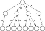
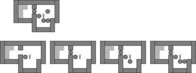
Without mentioning them, most implementations of memory-restricted search algorithms perform already a basic form of pruning; when the successors of a node are generated, they prohibit using an inverse action to return to the node's parent. For example, in an infinitely large Gridworld state space (see Fig. 10.1, left) with actions U, D, L, and R, the action sequence LR will always produce a duplicate node. Rejecting inverse action pairs, including RL, UD, and DU as well, reduces the number of children of a search node from four to three (see Fig. 10.1, middle).
 |
| Figure 10.1 |
In this section, we describe a method for pruning duplicate nodes that extends on this idea. The approach is suitable for heuristic search algorithms like IDA* that have imperfect duplicate detection due to memory restrictions; it can be seen as an alternative to the use of transposition or hash tables.
We take advantage of the fact that the problem spaces of most combinatorial problems are described implicitly, and consider the state space problem in labeled representation, so that Σ is the set of different action labels. The aim of substring pruning is to prune paths from the search process that contain one of a set of forbidden words D over Σ*. These words, called duplicates, are forbidden because it is known a priori that the same state can be reached through a different, possibly shorter, action sequence called a shortcut; only the latter path is allowed.
To distinguish between shortcuts and duplicates, we impose a lexicographical ordering ≤l on the set of actions in Σ. In the Gridworld example, it is possible to further reduce the search according to the following rule: Go straight in the x-direction first, if at all, and then straight in the y-direction, if at all, making at most one turn. Rejecting the duplicates DR, DL, UR, and UL (with respective shortcuts RD, LD, RU, and LU) from the search space according to this rule leads to the state space of Figure 10.1 (right). As a result, each point (x, y) in the Gridworld example is generated via a unique path. This reduces the complexity of the search tree to an optimal number of nodes (quadratic in the search depth), an exponential gain. The set of pruning rules we have examined depends on the fact that some paths always generate duplicates of nodes generated by other paths.
How can we find such string pairs (d, c), where d is a duplicate and c is a shortcut, and how can we guarantee admissible pruning, by means that no optimal solution is rejected?
First, we can initially conduct an exploratory (e.g., breadth-first) search up to a fixed-depth threshold. A hash table records all encountered states. Whenever a duplicate is indicated by the hash conflict, the lexicographically larger action sequence is recorded as a duplicate.
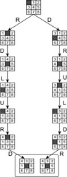
Another option that is applicable in undirected search spaces is to search for cycles, comparing a newly generated node in the search tree with all nodes in its generating path. The resulting cycle is split into one (or many) duplicate and shortcut (pairs). For example, the cycle in the (n2 − 1)-Puzzle RDLURDLURDLU with inverse DRULDRULDRUL is split as shown in Table 10.1. When splitting a full-length cycle, one part has to be inverted (all its actions have to be reversed). In case the length of one string is equal to the length of the other, we need some further criteria to draw a distinction between the two. One valid option is a lexicographic order on the set of actions Σ (and subsequently on the set of action strings Σ*). For actions Σ = {U, R, D, L}, let U ≤l R ≤l D ≤l L. The problem graph is undirected, so that we impose L to be inverse to R (written as L−1 = R), and U to be inverse to D. For RDLURDLURDLU and duplicate DRULDR, we have RDLURD as its corresponding shortcut. The example is illustrated in Figure 10.2.
For generating cycles, a heuristic can be used that minimizes the distance back to the initial state, where the search was invoked. For such cycle-detecting searches, state-to-state estimates like the Hamming distance on the state vector are appropriate.
The setting for unit-cost state space graphs naturally extends to weighted search spaces with a weight function w on the set of action strings as follows.
Definition 10.1
(Pruning Pair) Let G be a weighted problem graph with action label set Σ and weight function w: Σ* → ℝ. A pair (d, c) ∈ Σ* × Σ* is a pruning pair if:
1. w(d) > w(c), or, if w(d) = w(c), then c ≤l d;
2. for all u ∈ S: d is applicable in u if and only if c is applicable in u; and
3. for all u ∈ S we have that applying d on S yields the same result as applying c on S, if they are both applicable; that is, d(u) = c(u).
For sliding-tile puzzles, the applicability of an action sequence (condition 2) merely depends on the position of the blank. If in c the blank moves a larger distance in the x- or y-direction than in d, it cannot be a shortcut; namely, for some positions, d will be applicable, but not c. An illustration is provided in Figure 10.3. If all three conditions for a pruning pair are valid the shortcut is no longer needed and the search refinement can rely only on the duplicates found, which in turn admissibly prune the search. It is easy to see that truncating a path that contains d preserves the existence of an optimal path to a goal state (see Exercises).
 |
| Figure 10.3 |
The conditions may have to be checked dynamically during the actual search process. If conditions 2 or 3 are violated, we have to test the validity of a proposed pair (d, c). Condition 2 is tested by executing the sequence d−1c at every encountered state, and condition 3 is tested via comparing the respective states before and after executing d−1c.
Note that the state space does not have to include inversible actions to apply d−1 for testing conditions 2 and 3. Instead, we can use |d−1| parent pointers to climb up the search tree starting with the current state.
Pruning Automata
Assuming that we do not have to check conditions 2 or 3 for each encountered state, especially for depth-first, oriented search algorithms like IDA*, searching for a duplicate in the (suffix of the) current search tree path can slow down the exploration considerably, if the set of potential duplicates is large.
The problem of efficiently finding any of a set of strings in a text is known as the bibliographic search problem; it can be elegantly solved by constructing a substring acceptor in the form of a finite-state automaton, and feeding the text to it.
The automaton runs synchronous to the original exploration and prunes the search tree if the automaton reaches an accepting state. Each ordinary transition induces an automaton transition and vice versa. Substring pruning is important for search algorithms like IDA*, since constant-time pruning efforts fit well with enhanced DFS explorations. The reason is that the time to generate one successor for these algorithms is already reduced to a constant in many cases.
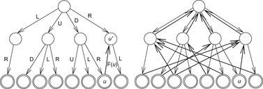
As an example, Figure 10.4 (left) shows the automaton for subset pruning with the string DU. The initial state is the most-left state and the accepting state is the most-right state in the automaton. Figure 10.4 (right) depicts the automaton for full predecessor elimination with accepting states omitted.
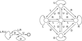
Table 10.2 shows the impact of substring pruning in the (n2 − 1)-Puzzle and in Rubik's Cube (see Ch. 1). Note that the branching factor 13.34 for the Rubik's Cube is already the result of substring pruning from the naïve space with a branching factor of 18, and the branching factors for the (n2 − 1)-Puzzle are already results of predecessor elimination (see Ch. 5). Different construction methods have been applied: BFS denotes that the search algorithm for generating duplicates operates breadth-first, with a hash conflict denoting the clash of two different search paths. An alternative method to find duplicates is cycle-detecting heuristic best-first search (CDBF). By unifying the generated sets of duplicates, both search methods can be applied in parallel (denoted as BFS + CDBF). We display the number of states in the pruning automaton and the number of duplicate strings that are used as forbidden words for substring matching.
As pruning strategies cut off branches in the search tree, they reduce the average node branching factor. We show this value with and without substring pruning (assuming that some basic pruning rules have been applied already).
Substring pruning automata can be included in the prediction of the search tree growth (see Ch. 5). This is illustrated in Figure 10.5 for substring pruning the grid by eliminating predecessors. In the beginning (depth 0) there is only one state. In the next iteration (depth 1) we have 4 states, then 6 (depth 2), 8 (depth 3), 10 (depth 4), and so on.
To accept several strings m1, …, mn, one solution is to construct a nondeterministic automaton that accepts them as substrings, representing the regular expression Σ*m1 Σ*|Σ* m2 Σ*| ⋯ |Σ* mn Σ*, and then convert the nondeterministic automaton into a deterministic one. Although this approach is possible, the conversion and minimization can be computationally hard.
Aho-Corasick Algorithm
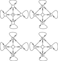
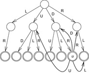
The algorithm of Aho and Corasick constructs a deterministic finite-state machine for a number of search strings. It first generates a trie of the set of duplicate strings. Figure 10.6 shows a trie for the duplicates in the Gridworld state space at depth 2. Every leaf corresponds to one forbidden action sequence and is considered to be accepting.
In the second step, the algorithm computes a failure function on the set of trie nodes. Based on the failure function, substring search will be available in linear time. Let u be a node in the trie and string(u) the corresponding string. The failure node failure(u) is defined as the location of the longest proper suffix of string(u), which is also the prefix of a string in the trie (see Fig. 10.7, bold arrows).
The failure values are computed in a complete breadth-first traversal, where, inductively, the values in depth i rely on the values computed in depth j < i. Algorithm 10.1 shows the corresponding pseudo code. To highlight the different branching in a search tree and in a trie, we use T(u, a) to denote a possible successor of u via a and write ⊥ if this successor along a is not available.
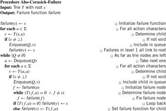
First, all nodes in BFS level 1 are determined and inserted into the queue Q. For the example this includes the four nodes in depth 1. As long as Q is nonempty, the top element u is deleted and its successors v are processed. To compute failure(v), the node in the sequence failure(u), failure2(u), failure3(u) is determined, which enables a transition with the chosen character a. As a rationale, if string(failure(u)) is the longest suffix of string(u) in the trie, and failure(u) has a child transition available labeled a, then string(failure(u))a is the longest suffix of string(u) that is contained in the trie.
In the example, to determine the failure value for node u in level 2 that was generated due to applying action R we go back via the link of its predecessor to the root node s and take the transition labeled R to u′. As a consequence, failure(u) = u′.
Each node is processed only once. Assuming the size of the alphabet to be bounded by a constant with an amortized analysis, we can show that computing the failure function takes time O(d) in total, where d is the sum of string lengths in D, d = ∑m ∈ D|m|.
Theorem 10.1
(Time Complexity of Failure Computation) Let D be the set of duplicates and d be the total length of all strings in D. The construction of the failure function is O(d).
Proof
Let |string(failure(u))| be the length of the longest proper suffix of string(u), that is prefix of one string in D, where a string is proper if it is not empty. If u′ and u are nodes on the path from the root node to a node i in T and u′ is the predecessor of u we have |string(failure(u))| ≤ |string(failure(u′))| + 1.
Choose any string mi that corresponds to a path pi in the trie for D. Then the total increase in the length for the failure function values of mi is ∑u ∈ pi |string(failure(u))| − |string(failure(u′))| ≤ |mi|. On the other side, |string(failure(u))| decreases on each failure transition by at least one and remains nonnegative throughout. Therefore, the total increase of the failure function strings for u on pi is at most |mi|.
To construct the substring pruning automaton A from T, we also use breadth-first search, traversing the trie T together with its failure function. In other words, we have to compute ΔA(u, a) for all automaton states u and all actions a in Σ. The skeleton of A is the trie T itself. The transitions ΔA(u, a) for u ∈ T and a ∈ Σ that are not in the skeleton can be derived from the function failure as follows. At a given node u we execute a at failure(u) using the already computed values of ΔA(failure(u), a). In the example, we have included the transitions for node u in Figure 10.8. The time complexity to generate A is O(d).
Searching existing substrings of a (path) string of length n is available in linear time by simply traversing automaton A. This leads to the following result.
Theorem 10.2
(Time Complexity Substring Matching) The earliest match of k strings of total length d in a text of length n can be determined in time O(n + d).
Automaton A can now be used for substring pruning as follows. With each node in the search process, we store a value state(u), denoting the state in the automaton; since A has d states, this requires about lg2d memory bits per state. If u has successor v with an action that is labeled with a we have state(v) = ΔA(a, s). This operation is available in constant time. Therefore, we can check in constant time if the generating path to u has one duplicate string as a suffix.
*Incremental Duplicate Learning A*
A challenge is to apply substring pruning dynamically, during the execution of a search algorithm. In fact, we have to solve a variant of the dynamic dictionary matching problem. Unfortunately, the algorithm of Aho and Corasick is not well suited to this problem.
In contrast to the static dictionary approach to prune the search space, generalized suffix trees (as introduced in Ch. 3) make it possible to insert and delete strings while maintaining a quick substring search. They can be adapted to a dictionary automaton as follows.
For incremental duplicate pruning with a set of strings, we need an efficient way to determine Δ(q, a) for a state q and action character a, avoiding the reconstruction of the path to the current state in the search tree.
Theorem 10.3
(Generalized Suffix Trees as FSMs) Let string a be read from a1 to aj − 1. There is a procedure Δ for which the returned value on input aj is the longest suffix ai, …, aj of a1, …, aj that is also the substring of one string m stored in the generalized suffix tree. The amortized time complexity for Δ is constant.
Proof
An automaton state q in the generalized suffix tree automaton is a pair q = (i, l) consisting of the extended locus l and the current index i on the contracted edge incident to l. Recall that substrings referred to at l are denoted as intervals [first, last] of the strings stored.
To find q′ = Δ(q, a) starting at state (i, l) we search for a new extended locus l′ and a new integer offset i′, such that a corresponds to the transition stored at index position first + i of the substring stored at l. We use existing suffix links of the contracted loci and possible rescans if the character a does not match, until we have found a possible continuation for a. The extended locus of the edge and the reached substring index i′ determines the pair (l′, i′) for the next state. In case of reaching a suffix tree node that corresponds to a full suffix we have encountered an accepting state q*. The returned value in q* is the substring corresponding to the path from the root to the new location. By amortization we establish the stated result.
For a dynamic learning algorithm, we interleave duplicate detection with A*. As A* already has full duplicate detection based on states stored in the hash table, using substring pruning is optional. However, by following this case, it is not difficult to apply dynamic subset pruning to other memory-restricted search algorithms. For the sake of simplicity, we also assume that the strings m stored in the generalized suffix tree are mutually substring free; that is, no string is a substring of another one.
The resulting algorithm is denoted as incremental duplicate learning A* (IDLA*). Its pseudo code is shown in Algorithm 10.2. As usual, the update of the underlying data structures Open and Closed are hidden in the call of Improve, which mainly implements the relaxation step f(v) ← {f(v), f(u) + w(u, v)}. The algorithm takes a state space problem and a (empty or preinitialized) dictionary automaton data structure D as input parameters. If according to the assumed regularity of the search space the detected tuples (d, c) are pruning pairs, we only have to store string d. If we are uncertain about the regularity at the accepting state of the dictionary automaton for d, we additionally store the proposed shortcut c and check whether or not it is actually applicable. Either way, inherited by the optimality of A*, the search algorithm outputs an optimal solution path.
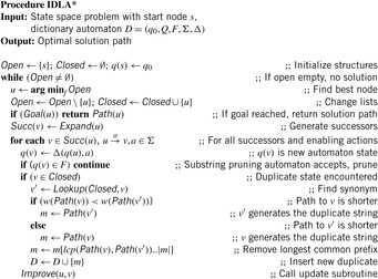
The algorithm provides combined duplicate detection and usage. Before searching a node in the hash table, we search if we encounter an accepting state in D. Depending on the regularity of the search space, we might or might not check whether the proposed shortcut is valid. If D does not accept, then we use the hash table to find a synonym v′ of the successor node v of u. If we do not find a match then we insert the new node in the ordinary search structures only.
If there is a counterpart v′ of v in the hash table for Closed (computed using the generic Lookup procedure; see Ch. 3), we prune the longest common prefix (lcp) of both generating paths to construct the pair (d, c). This is useful to enhance the generality and pruning power of (d, c). The shorter the strings, the larger the potential for pruning. The correctness argument is simple: If (d, c) is a pruning pair, then every common prefix extension is also a pruning pair. As a result the reduced pair is inserted into the dictionary.
For a simple example we once more consider the Gridworld. As a heuristic we choose the Manhattan distance estimate. Suppose that the algorithm is invoked with initial state (3, 3) and goal state (0, 0). Initially, we have Open = {((3, 3), 6)}, where the first entry denotes the state vector in the form of a Gridworld location and the second entry denotes its heuristic estimate. Expanding the initial states yields the successor set {((4, 3), 8), ((3, 4), 8), ((3, 2), 6), ((2, 3), 6)}. Since no successor is hashed, all elements are inserted into Open and Closed. In the next step, u = ((2, 3), 6) is inserted and one successor v = ((3, 3), 8) turns out to have a counterpart v′ = ((3, 3), 6) in the hash table. This leads to the duplicate LR with corresponding shortcut ϵ, which is inserted into the dictionary automaton data structure. Next, ((3, 2), 6) is expanded. We establish another duplicate string DU with shortcut sequence ϵ. Additionally, we encounter the pruning pair (LD, DL), and so on.
10.1.2. Pruning Dead-Ends
In domains like the Fifteen-Puzzle, every configuration that we can reach by executing an arbitrary move sequence remains solvable. This is not always the case, though. In several domains there are actions that can never be reversed (doors may shut if we go through). This directly leads to situations where a solution is out of reach.
A simple case of a dead-end in Sokoban can be obtained by pushing a ball into a corner, from where it cannot be moved. The goal of dead-end pruning is to recognize and avoid these branches as early as possible. There is, of course, an exception since a ball in a corner is a dead-end if and only if the corner position is not a goal field. In the following we exclude this subtle issue from our considerations.
This section presents an algorithm that allows us to generate, memorize, and generalize situations that are dead-ends. The strategy of storing unsolvable subpositions is very general, but to avoid introducing extensive notation, we take the Sokoban problem (see Ch. 1) as a welcome case study.
Two simple ways of identifying some special cases of dead-end positions in Sokoban can be described by the two procedures IsolatedField and Stuck. The former one checks for one or two connected, unoccupied fields that are surrounded by balls and not reachable by the man without pushes. If it is not possible to connect the squares only by pushing the surrounding balls “from the outside,” the position one is a dead-end. The latter procedure, Stuck, checks if a ball is free; that is, if it has either no horizontal neighbor or no vertical neighbor. Initially, place all nonfree balls into a queue. Then, ignoring all free balls, iteratively try to remove the free balls from the queue until it becomes empty or nothing changes anymore. If in one iteration every ball stays inside the queue, some of which are not located on goal fields, the position is a dead-end. In the worst case, Stuck needs O(n2) operations for n balls, but in most cases it turns out to operate in linear time. The correctness is given by the fact that to free a ball with the men from a given position at least two of its neighbors have to be free.
Figure 10.9 illustrates the procedure and shows an example of a dead-end in Sokoban. Balls 1, 2, 5, or 6 cannot be moved, but balls 3, 4, 7, and 8 can be moved. It is obvious that without detecting the dead-end already on these balls, this position can be the root of a very large search tree. Initially all balls are put in a queue. If a ball is free it is removed, otherwise it is enqueued again. After a few iterations we reach a fixpoint. Balls 1, 2, 5, and 6 cannot be set free. Such a position is a valid end state only if the balls are correctly placed on goal fields.

We could perform these checks prior to every node expansion. Note, however, that they provide only sufficient but not necessary conditions for dead-ends. We can strengthen the pruning capabilities based on the following two observations:
• A dead-end position can be recursively defined as being either a position that can be immediately recognized as a dead-end, or a nongoal position in which every move that is available leads to a dead-end position. If all successors of a position are dead-ends, the position itself is a dead-end as well.
• Many domains allow a generalization of dead-end patterns; we can define a relation ⊑ and write v ⊑ u if v is a subproblem of u. If v is not solvable, then neither is u. For example, a (partial) dead-end Sokoban position remains a dead-end if we add balls to it. Thus, ⊑ turns out to be a simple pattern matching relation.
Decomposing a problem into parts has been successfully applied in divide-and-conquer algorithms, and storing solutions to already solved subproblems is called memorizing. The main difference to these approaches is that we concentrate on parts of a position to be retrieved. For Sokoban, decomposing a position should separate unconnected positions and remove movable balls to concentrate on the intrinsic patterns that are responsible for a dead-end. For example, in Figure 10.9 the position can be decomposed by splitting the two ball groups. The idea of decomposing a position is a natural generalization of the isolated field heuristic: A position with nongoal fields on which the man can never get is a likely dead-end. Take the graph G of all empty squares and partition G into connected components (using linear time). Examine each component separately. If every empty square can be reached by the man the position is likely to be alive. If one component is a dead-end, and indeed often they are, the entire position itself is a dead-end.
Our aim is to learn and generalize dead-end positions when they are encountered in the search; some authors also refer to this aspect as bootstrapping. Each dead-end subproblem found and inserted into the subset dictionary (see Ch. 3) can be used immediately to prune the search tree and therefore to get deeper into the search tree.
Depending on the given resources and heuristics, decomposition could be either invoked in every expansion step, every once in a while, or only in critical situations. The decomposition itself has to be carefully chosen to allow a fast dead-end detection and therefore a shallow search. A good trade-off has to be found: The characteristics responsible for the dead-end on one the hand should appear in only one component and, on the other hand, the problem parts should be far more easy to analyze than the original one. For Sokoban, we can consider the partial position that consists of all balls that cannot be safely removed by the procedure Stuck.
Before we turn to the implementation, we study the search tree for the Sokoban puzzle shown in Figure 10.10. It demonstrates how the preceding two observations, in conjunction with a simple dead-end detection, can use bottom-up propagation to generalize more complex patterns.
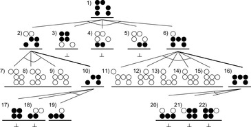
The root position s is a dead-end, and although the IsolatedField procedure would immediately recognize this, we assume for the sake of the argument that only Stuck is used as the basic dead-end position detection. Initially, the subset dictionary is empty and the status of s is undefined. We expand u and generate its successor set Succ(u). Three of the five elements in Succ(u) are found to be a dead-end; the responsible balls are marked as filled circles. Marking can be realized through a Boolean array, with true denoting that the corresponding ball is relevant for the dead-end, and false otherwise. For usual transitions, a ball is a necessary constituent of a dead-end pattern if it is responsible for the unsolvability of one successor state; hence, unifying the relevant vectors is done by a Boolean or-operation. Generally, a state u is a dead-end if relevant(u) ⊑ u is a dead-end. Initially, relevant is the constantly false function for all states.
Since in this instance the status of two successors is not defined, overall solvability remains open. Therefore, the left-most and right-most nodes are both expanded (thin edges) and decomposed (bold edges). Decomposition is preferred, which is done by assigning a g-value of zero to the newborn child.
The expansion of the partial states is easier, and we find all of their successors dead-ended within one more step. As the root is a dead-end, we want to find a minimal responsible pattern by means of backpropagation. By unification, we see that all balls of the expanded nodes in the second-to-last level are relevant. Both positions are newly found dead-ended and inserted into the subset dictionary. Since we have now reached a decomposition node, it is sufficient to copy the relevant part to the parent; the failure of one component implies the failure of the complete state. All generated nodes in Succ(u) are dead-ends, and we can further propagate our knowledge bottom-up by forming the disjunction of the successor's relevance information. Finally, the root is also inserted into the subset dictionary.
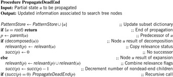
The corresponding pseudo code for this kind of bottom-up propagation is given in Algorithm 10.3. We assume that in addition to the vector of flags relevant, each node maintains a counter succ of the number of nondead-end children.
The main procedure Abstraction-Decomposition-A* (see Alg. 10.4) carries out the search for solvability (of possibly decomposed states) and for an optimal solution (in the main search tree) in an interleaved fashion; a flag decomposed(u) remembers which of the two modes is currently applied to state u. Moreover, solvable(u) keeps track of its status: true, false, or unknown.
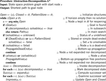
Like in A*, until the priority queue gets empty, the node with the best f-value is selected. If it is a goal node and we are in the top search level, we have found the solution to the overall problem and can terminate; otherwise, the partial position is obviously solvable. For nongoal nodes, we try to establish their solvability by applying a simple dead-end check (e.g., using procedure Stuck), or by recognizing a previously stored pattern. Unsolvable partial positions are used to find larger dead-end patterns by backpropagation, as described earlier.
Since we are only interested in solvability of decomposed nodes, we do not have to search the subproblems all the way to the end. If we have enough information for a subproblem to be alive, we can back up this knowledge in the search tree in an analogous way. We might also allow a one-sided error without harming overall admissibility (i.e., let the alive procedure be overly optimistic).
The main difference to usual A* search is that for a node expansion of u, in addition to the set of successor nodes Succ(u), decomposed positions Δ(u) are generated and then inserted into Open with g set to zero to distinguish the new root from other search tree nodes. The ordinary successors are inserted, dropped, and reopened as usual in A*. Instead of using a lower-bound estimate h to solve the puzzle, in the learning process we can also try to actively focus the search to produce dead-ends.
Efficiently storing and searching dead-end (sub)positions is central to the whole learning process. We have called the abstract data structure providing insertion and lookup of substructures a pattern store. Possible implementations of such a dictionary data structure have been provided in Chapter 3.
10.1.3. Penalty Tables
In this section, an approach related to Abstraction-Decomposition-A* is described that tries to generalize, store, and reuse minimal dead-end patterns as well, but uses auxiliary, separate pattern searches instead of a dedicated decomposition/generalization procedure.
The approach can be conveniently described for the Sokoban domain. We refer to two different mazes: the original maze (i.e., the maze containing all the balls of the current position) and the test maze, which will be used for pattern searches. The pattern search algorithm's design is iterative and starts when a dead-end position has been found. Only the last ball moved is put into the test maze, and the algorithm tries to solve this simplified problem. If it succeeds, another A* test search is triggered, with some other ball of the original maze added; those balls are preferred that interfere with the path of the man or of a ball in the previous solution. If no solution is found, a dead-end is detected. An example is provided in Figure 10.11. Since this pattern need not yet to be minimal, successive iterations try to remove one ball at a time while preserving the dead-end property.
 |
| Figure 10.11 |
To fine-tune the trade-off between main and auxiliary search, a number of parameters control the algorithm, such as the maximum number of expansions maxn in each individual pattern search, the maximal pattern size maxb, and the frequency of pattern searches. One way to decide on the latter one is to trigger a pattern search for each position if the number of its descendants explored in the main search exceeds a certain threshold.
To improve search efficiency, we can make some further simplifications to the A* procedure: Since the pattern search is only concerned with solvability, as a heuristic it suffices to consider each ball's shortest distance to any goal field rather than computing a minimal matching, as usual. Moreover, balls on goal fields or balls that are reachable and free and can be immediately removed.
We can regard a dead-end subset dictionary as a table that associates each matching position with a heuristic value of ∞. This idea leads to the straightforward extension of dead-end detection to penalty tables, which maintain a corrective amount by which the simpler, procedural heuristic differs from the true goal distance. When a partial position has actually turned out to be solvable, the found solution distance might be larger than the standard heuristic indicates; in other words, the latter one is wrong. Multiple corrections from more than one applicable pattern can be added if the patterns do not overlap. Again, possible implementations for penalty tables are subset dictionaries as discussed in Chapter 3.
To apply pattern search in other domains, two properties are required: reducibility of the heuristic and splittability of the heuristic with regard to the state vector. These conditions are defined as follows. A state description S (viewed as a set of values) is called splittable, if for any two disjoint subsets S1 and S2 of S we have δ(S) = δ(S1) + δ(S2) + δ(S (S1 ∪ S2)) + C; this means that the solution of S is at least as long as both subsolutions added. The third term accounts for additional steps that might be needed for conditions that are neither in S1 nor in S2, and C stands for subproblem interactions. A heuristic is reducible, if h(S′) ≤ h(S) for S′ ⊆ S. A heuristic is splittable, if for any two disjoint subsets S1 and S2 of S we have h(S) = h(S1) + h(S2) + h(S (S1 ∪ S2)). The minimum matching heuristic introduced in Chapter 1 is not splittable but the sum of the distances to the closest goal results in a splittable heuristic.
If a heuristic is admissible, for S′ ⊆ S we additionally have a possible gap δ(S′) − h(S′) ≥ 0. We define the penalty with respect to S′ as pen(S′) = δ(S′) − h(S′).
Theorem 10.4
(Additive Penalties) Let h be an admissible, reducible, and splittable heuristic; S be a state set; and S1, S2 ⊆ S be disjoint subsets of S. Then we have pen(S) ≥ pen(S1) + pen(S2).
Proof
Using admissibility of h and the definition of penalties, we deduce
As a corollary, the improved heuristic h′(S) = h(S) + pen(S1) + pen(S2) is admissible since h′(S) ≤ h(S) + pen(S) = δ(S). In other words, assuming reducibility and splittability for the domain and the heuristic, the penalties of nonoverlapping patterns can be added without affecting admissibility.
Pattern search was one of the most effective techniques for solving many Sokoban instances. It has also been used to improve the performance of search in the sliding-tile puzzle domains. In the Fifteen-Puzzle the savings in the number of nodes are of about three to four orders of magnitude of difference compared to the Manhattan distance heuristic.
10.1.4. Symmetry Reduction
For multiple lookups in pattern databases (see Ch. 4), we already utilized the power of state space symmetries for reducing the search efforts. For every physical symmetry valid in the goal we apply it to the current state and get another estimate, which in turn can be larger than the original lookup and lead to stronger pruning. In this section, we expand on the observation and embed the observation in a more general context.
As a motivating example of the power of state space reduction through existing symmetries in the problem description, consider the Arrow Puzzle problem, in which the task is to change the order of the arrows in the arrangement  to
to  , where the set of allowed actions is restricted to reversing two adjacent arrows at a time. One important observation for a fast solution to the problem is that the order of arrow reversal does not matter. This exploits a form of action symmetry that is inherent in the problem. Moreover, two outermost arrows don't participate in an optimal solution and at least three reversals are needed. Therefore, any permutation of swapping the arrow index pairs (2,3), (3,4), and (4,5) leads to an optimal solution for the problem.
For state space reduction with respect to symmetries we expect to be provided by the domain expert, we use equivalence relations. Let P = (S, a, s, T) be a state space problem as introduced in Chapter 1.
Definition 10.2
(Equivalence Classes, Quotients, Congruences) A relation ∼ ⊆ S × S is an equivalence relation if the following three conditions are satisfied: ∼ is reflexive (i.e., for all u in S we have u ∼ v); ∼ is symmetric (i.e., for all u and v in S we have if u ∼ v then v ∼ u); and ∼ is transitive (i.e., for all u, v, and w in S we have u ∼ v and v ∼ w implies u ∼ w). Equivalence relations naturally yield equivalence classes [u] = {v ∈ S | u ∼ v} and a (disjoint) partition of the search space into equivalence classes S = [u1] ∪ ⋯ ∪ [uk] for some k. The state space (S/∼) = {[u] | u ∈ S} is called quotient state space. An equivalence relation ∼ of S is a congruence relation on P if for all u, u′ ∈ S with u ∼ u′ and action a ∈ A with a(u) = v, there is a v′ ∈ S with v ∼ v′ and an action a′ ∈ A with a′(u′) = v′. Any congruence relation induces a quotient state space problem (P/∼) = (S/∼), (A/∼), [s], {[t] | t ∈ T}). In (P/∼) an action [a] ∈ (A/∼) is defined as follows. We have [a]([u]) = [v] if and only if there is an action a ∈ A mapping u to v so that u ∈ [u] and v′ ∈ [v′].
Note that (A/∼) is sloppy in saying that the congruence relation ∼ partitions the action space A.
Definition 10.3
(Symmetry) A bijection ϕ: S → S is said to be a symmetry if ϕ(s) = s, ϕ(t) ∈ T for all t ∈ T and for any successor v to u there exists an action from ϕ(u) to ϕ(v). Any set Y of symmetries generates a subgroup g(Y) called a symmetry group. The subgroup g(Y) induces an equivalence relation ∼Y on states, defined as u ∼Y v if and only if ϕ(u) = v and ϕ ∈ g(Y). Such an equivalence relation is called a symmetry relation on P induced by Y.
Any symmetry relation on P is a congruence on P. Moreover, u is reachable from s if and only if [u]Y is reachable from [s]Y. This reduces the search for goal t ∈ T to the reachability of state [t]Y.
To explore a state space with respect to a state symmetry, we use a function Canonicalize each time a new successor node is generated, which determines a representative element for each equivalence class. Note that finding symmetries automatically is not easy, since it links to the computational problem of graph isomorphism, which is hard.
If a symmetry is known, then the implementation of symmetry detection is immediate, since both the Open set and Closed set can simply maintain the outcome of the Canonicalize action.
One particular technique for finding symmetries is as follows. In some search problems states correspond to (variable) valuations and goals are specified with partial valuations. Actions are often defined transparent to the assignments of values to the variables. For example, an important feature of (parametric) planning domains is that actions are generic to bindings of the parameters to the objects.
As a consequence, a symmetry in the form of a permutation of variables in the current and in the goal state has no consequence to the set of parametric actions.
Let V be the set of variables with |V| = n. There are n! possible permutations of V, a number likely too large to be checked for symmetries. Taking into account type information on variable types reduces the number of all possible permutations of the variables to  , where ti is the number of variables with type i, i ∈ {1, …, k}. Even for moderately sized domains, this number is likely still too large. To reduce the number of potential symmetries to a tractable size, we further restrict symmetries to variable transpositions [v ↔ v′] (i.e., a permutation of only two variables v, v′ ∈ V), for which we have at most n(n − 1)/2 ∈ O(n2) candidates. Using type information this number reduces to
  , which often is a practical value for symmetry detection.
, where ti is the number of variables with type i, i ∈ {1, …, k}. Even for moderately sized domains, this number is likely still too large. To reduce the number of potential symmetries to a tractable size, we further restrict symmetries to variable transpositions [v ↔ v′] (i.e., a permutation of only two variables v, v′ ∈ V), for which we have at most n(n − 1)/2 ∈ O(n2) candidates. Using type information this number reduces to We denote the set of (typed) variable transpositions by M. The outcome of a transposition of variables (v, v′) ∈ M applied to a state u = (v1, …, vn), written as u[v ↔ v′], is defined as (v′1, …, v′n), with v′i = vi if vi ∉ {v, v′}, vi = v′ if vi = v, and vi = v if vi = v′. It is simple to extend the definition to parametric actions.
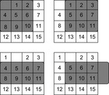
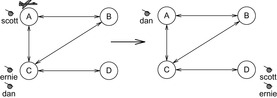
In the example depicted in Figure 10.12, we have variables denoting the location of persons, so that we can write We observe that u[v ↔ v′] = u[v′ ↔ v] and u[v ↔ v′][v ↔ v′] = u.
 |
| Figure 10.12 |
Theorem 10.5
(Time Complexity for Object Symmetry Detection) The worst-case complexity to determine the set of all variable transpositions for which a problem P = (S, A, s, T) is symmetric is bounded by O(|M| ⋅ n) operations.
Proof
A state space problem P = (S, A, s, T) is symmetric with respect to the transposition [v ↔ v′], abbreviated as P[v ↔ v′], if s[v ↔ v′] = s and T[v ↔ v′] ∈ T. The brute-force time complexity for computing u[v ↔ v′] is of order O(n). However, by precomputing a lookup table containing the index of u′ = u[v ↔ v′] for all (v, v′) ∈ M, this complexity can be reduced to one lookup.
For the example problem, the goal contains the three target locations of dan, ernie, and scott. In the initial state the problem contains no symmetry, since s[scott ↔ ernie] ≠ s and T[dan ↔ ernie] ≠ T. In forward-chaining search, which explores the search space starting in a forward direction starting with the initial state s, symmetries that are present in s may vanish or reappear. Goals, however, do not change over time. Therefore, in an offline computation we can refine the set of symmetries M to M′ = {(v, v′) ∈ M | T[v ↔ v′] = T. Usually, |M′| is much smaller than |M|. For the example problem instance, the only variable symmetry left in M′ is the transposition of scott and ernie. The remaining task is to compute the set M″(u) = {(v, v′) ∈ M′ | u[v ↔ v′] = u} of symmetries that are present in the current state u. In the initial state s of the example problem, we have M″(s) = ∅, but once scott and ernie share the same location in a state u, this variable pair is included in M″(u). With respect to Theorem 10.5 this additional restriction reduces the time complexity to detect all remaining variable symmetries to O(|M′| ⋅ n).
If a state space problem with current state c ∈ S is symmetric with respect to the variable transposition [v ↔ v′] then applications of actions are neglected, significantly reducing the branching factor. The pruning set A′(u) of a set of applicable actions A(u) is the set of all actions that have a symmetric counterpart and that are of minimal index.
Theorem 10.6
(Optimality of Symmetry Pruning) Reducing the action set A(u) to A′(u) for all states u during the exploration of state space problem P = (S, A, s, T) preserves optimality.
Proof
Suppose that for some expanded state u, reducing the action set A(u) to A′(u) during the exploration of planning problem P = (S, A, s, T) does not preserve optimality. Furthermore, let u be the state with this property that is maximal in the search order. Then there is a solution π = (a1, …, ak) in Pu = (S, A, u, T) with associated state sequence (u0 = u, …, uk ⊆ T). Obviously, ai ∈ a(ui − 1), i ∈ {1, …, k}. By the definition of the pruning set there exists a′1 = a1[v ↔ v′] of minimal index that is applicable in u0.
Since Pu = (S, A, u, T) = Pu[v ↔ v′] = (S, A, u[v ↔ v′] = u, T[v ↔ v′] = T), we have a solution a1[v ↔ v′], …, ak[v ↔ v′] with state sequence (u0[v ↔ v′] = u0, u1[v ↔ v′], …, uk[v ↔ v′] = uk) that reaches the goal T with the same cost. This contradicts the assumption that reducing the set A(u) to A′(u) does not preserve optimality.
10.2. Nonadmissible State Space Pruning
In this section we consider different options for such reasoning that sacrifice solution optimality but yield large reductions to the search efficiency.
10.2.1. Macro Problem Solving
In some cases it is possible to group a sequence of operators to build a new one. This allows the problem solver to apply many primitive operators at once. For pruning the new combined operators substitute the original ones so that we reduce the set of applicable operators for a state. The pruning effect is that the strategy requires fewer overall decisions when ignoring choices within each sequence. Of course, if the substitution of operators is too generous, then the goal might not be found.
Here, we consider an approach for the formation of combined operators that may prune the optimal solutions, but preserve the existence of at least one solution path. A macro operator (macro for short) is a fixed sequence of elementary operators executed together. More formally, for a problem graph with node set V and edge set E a macro refers to an additional edge e = (u, v) in V × V for which there are edges e1 = (u1, v1), …, ek = (uk, vk) ∈ E with u = u1, v = vk, and vi = ui + 1 for all 1 ≤ i ≤ k − 1. In other words, the path (u1, …, uk, vk) between u and v is shortcut by introducing e.
Macros turn an unweighted problem graph into a weighted one. The weight of the macro is the accumulated weight of the original edges,  . It is evident that inserting edges does not affect the reachability status of nodes. If there is no alternative in the choice of successors, Succ(ui) = {vi}, macros can simply substitute the original edges without loss of information. As an example, take maze areas of width one (tunnels) in Sokoban.
If there are more paths between a node, to preserve optimality of an underlying search algorithm, we have to take the shortest one, w(u, v) = δ(u, v). These macros are called admissible. The All-Pairs Shortest Paths algorithm of Floyd-Warshall (see Chapter 2) can be seen as one example of introducing admissible macros to the search space. At the end of the algorithm, all two nodes are connected (and assigned to the minimum path-cost value). The original edges are no longer needed to determine the shortest path value, such that omitting the original edges does not destroy the optimality of a search in the reduced graph.
Unfortunately, regarding the size of the search spaces we consider, computing All-Pairs Shortest Paths in the entire problem graph is infeasible. Therefore, different attempts have been suggested to approximate the information that is encoded in macros. If we are interested only in computing some solution, we can use inadmissible macros or delete problem graph edges after some but not all admissible macros have been introduced. The importance of macros in search practice is that they can be determined before the overall search starts. This process is called macro learning.
A way to use inadmissible macros is to insert them with a weight w(u, v) smaller than the optimum δ(u, v) such that they will be used with higher priority. Another option is to restrict the search purely to the macros, neglecting all original edges. This is only possible if the goal remains reachable.
In the rest of this section, we give an example on how a macro problem solver can transform a search problem into an algorithmic scheme: The problem is decomposed into an ordered list of subgoals, and for each subgoal, a set of macros is defined that transform a state into the next subgoal.
We take the Eight-Puzzle as an example. Again, actions are labeled by the direction in which the blank is moving. The entry in row r and column c in the macro table (see Table 10.3) holds the operator sequence to position the tile in position r into position c, such that after executing the macro at (r, c) the tiles in position 1 to r − 1 remain correctly placed.
Figure 10.13 shows the successive application of macro actions. For tile i, 1 ≤ i ≤ 6, its current location c and its goal location r are determined, and the corresponding macro is applied.
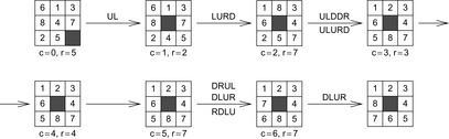
Given a macro table, we can estimate the worst-case solution length needed by the macro solver by summing the string size maxima in the columns. For the Eight-Puzzle we get a maximal length of 2 + 12 + 10 + 14 + 8 + 14 + 4 = 64. As an estimate for the average solution length, we can add the arithmetic means of the macro lengths in the columns, which yields
To construct the macro table, it is most efficient to conduct a DFS or BFS search in a backward direction, starting from each goal state separately. For this purpose we need backward operators (which do not necessarily need to be valid operators themselves).
The row r(m) of macro m is the position on which pc(m) is located, which has to be moved to c(m) in the next macro application. The inverse of macro m will be denoted as m−1.
For example, starting with the seventh subgoal, we will encounter a path m−1 = LDRU, which alters goal position p′ = (0, 1, 2, 3, 4, 5, 6, 7, 8) into p = (0, 1, 2, 3, 4, 5, 8, 6, 7). Its inverse is DLUR; therefore, c(m) = 6 and r(m) = 7, matching the last macro application in Figure 10.13.
10.2.2. Relevance Cuts
Humans can navigate through large state spaces due to an ability to use meta-level reasoning. One such meta-level strategy is to distinguish between relevant and irrelevant actions. They tend to divide a problem into several subgoals, and then to work on each subgoal in sequence. In contrast, standard search algorithms like IDA* always consider all possible moves available in each position. Therefore, it is easy to construct examples that are solvable by humans, but not by standard search algorithms. For example, in a mirror-symmetrical Sokoban position, it is immediately obvious that each half can be solved independently; however, IDA* will explore strategies that humans would never consider, switching back and forth between the two subproblems many times.
Relevance cuts attempt to restrict the way the search process chooses its next action, to prevent the program from trying all possible move sequences. Central to the approach is the notion of influence; moves that don't influence each other are called distant moves. A move can be cut off, if within the last m moves, more than k distant moves have been made (for appropriately chosen m and k); or, if it is distant to the last move, but not some move within the last m moves.
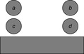
The definition of distant moves generally depends on the application domain; we sketch here one approach for Sokoban. First, we have to set up a measure for influence. We precompute a table for the influence of each square on each other one. The influence relation reflects the number of paths between the squares; the more alternatives exist, the less the influence. For example, in Figure 10.14 a and b influence each other less than c and d. Squares on the optimal path should have a stronger influence than others. Neighboring squares that are connected by a possible ball push are more influencing than if only the man can move between them. For example, in Figure 10.14 a influences c more than c influences a. In a tunnel, influence remains the same, regardless of the length of the tunnel. Note that the influence relation is not necessarily symmetric.
Given a relevance table, a move M2 is regarded as distant from a previous move M1, if its from-square influences M1's from-square by less than some threshold, θ.
There are two possible ways that a move can be pruned. First, if within the last set of k moves more than l distant moves were made. This cut discourages arbitrary switches between nonrelated areas of the maze. Second a move that is distant with respect to the previous move, but not distant to a move in the past k moves. This will not allow switches back into an area previously worked on and abandoned just before. If we set l = 1, the first criterion entails the second. Through the restrictions are imposed by relevance cuts, optimality of the solution can no longer be guaranteed. However, a number of previously unsolvable Sokoban instances could be handled based on this technique. To avoid pruning away optimal solutions, we can introduce randomness to the relevance cut decision. The probability determines if a cut is applied or not and reflects the confidence in the relevance cut.
Relevance cuts have been analyzed using the theoretical model of IDA* search (see Ch. 5). Unfortunately, in an empirical study the model turned out to be inadequate to handle the nonuniformity of the search space in Sokoban.
10.2.3. Partial Order Reduction
Partial order reduction methods exploit the commutativity of actions to reduce the size of the state space. The resulting state space is constructed in such a manner that it is equivalent to the original one. The algorithm for generating a reduced state space explores only some of the successors of a state. The set of enabled actions for node u is called the enabled set, denoted as enabled(u). The algorithm selects and follows only a subset of this set called the ample set, denoted as ample(u). A state u is said to be fully expanded when ample(u) = enabled(u), otherwise it is said to be partially expanded.
Partial order reduction techniques are based on the observation that the order in which some actions are executed is not relevant. This leads to the concept of independence between actions.
Definition 10.4
(Independent Actions) Two actions a1 and a2 are independent if for each state u ∈ S the following two properties hold:
1. Enabledness is preserved: a1 and a2 do not disable each other.
2. a1 and a2 are commutative: a(a′(u)) = a′(a(u)).
As a case study, we choose propositional Strips planning, where the planning goal is partially described by a set of propositions.
Definition 10.5
(Independent Strips Planning Actions) Two Strips planning actions a = (pre(a), add(a), del(a)) and a′ = (pre(a′), add(a′), del(a′)) are independent if del(a′) ∩ (add(a) ∪ pre(a)) = ∅ and (add(a′) ∪ pre(a′)) ∩ del(a) = ∅.
Theorem 10.7
(Commutativity of Independent Strips Actions) Two independent Strips actions are enabledness preserving and commutative.
A further fundamental concept is the fact that some actions are invisible with respect to the goal. An action α is invisible with respect to the set of propositions in the goal T, if for each pair of states u, v, if v = α(u), we have u ∩ T = v ∩ T.
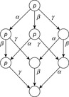
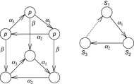
Figure 10.15 illustrates independence and invisibility of actions. Actions α, β, and γ are pairwise independent. Actions α and β are invisible with respect to the set of propositions T = {p}, but γ is not. The figure also illustrates why partial order reduction techniques are said to exploit diamond properties of a system.
The main goal of the ample set construction is to select a subset of the successors of a state such that the reduced state space is stuttering equivalent to the full state space with respect to a goal. The construction should offer a significant reduction without requiring a high computational overhead. Enough paths must be retained to give correct results. The following four conditions are necessary and sufficient for the proper construction of a partial order reduced state space for a given goal.
C0: ample(u) is empty exactly when enabled(u) is empty.
C1: Along every path in the full state space that starts at u, an action that is dependent on an action in ample(u) does not occur without an action in ample(u) occurring first.
C2: If a state u is not fully expanded, then each action α in the ample set of u must be invisible with regard to the goal.
C3: If for each state of a cycle in the reduced state space an action α is enabled, then α must be in the ample set of some of the successors of some of the states of the cycle.
The general strategy to produce a reduced set of successors is to generate and test a limited number of ample sets for a given state, which is shown in Algorithm 10.5. Conditions C0, C1, and C2 or their approximations can be implemented independently from the particular search algorithm used. Checking C0 and C2 is simple and does not depend on the search algorithm. Checking C1 is more complicated. In fact, it has been shown to be at least as hard as establishing the goal for the full state space. It is, however, usually approximated by checking a stronger condition that can be checked independently of the search algorithm. We shall see that the complexity of checking the cycle condition C3 depends on the search algorithm used.

Checking C3 can be reduced to detecting cycles during the search. Cycles can be easily established in depth-first search: Every cycle contains a backward edge, one that links back to a state that is stored on the search stack. Consequently, avoiding ample sets containing backward edges except when the state is fully expanded ensures satisfaction of C3 when using IDA*, since it performs a depth-first traversal. The resulting stack-based cycle condition C3stack can be stated as follows:
C3stack: If a state u is not fully expanded, then at least one action in ample(u) does not lead to a state on the search stack.
Consider the example on the left of Figure 10.16. Condition C3stack does not characterize the set {α1} as a valid candidate for the ample set. It accepts {α1, α2} as a valid ample set, since at least one action (α2) of the set leads to a state that is not on the search stack of the depth-first search.

The implementation of C3stack for DFS strategies marks each expanded state on the stack, so that stack containment can be checked in constant time.
Detecting cycles with general search algorithms that do not perform a depth-first traversal of the state space is more complex. For a cycle to exist, it is necessary to reach an already generated state. If during the search a state is found to be already generated, checking that this state is part of a cycle requires checking whether this state is reachable from itself. This increases the time complexity of the algorithm from linear to quadratic in the size of the state space. Therefore, the commonly adopted approach assumes that a cycle exists whenever an already generated state is found. Using this idea leads to weaker reductions. Fortunately for reversible state space the self-reachability check is trivial.
The cycle condition C3stack cannot be used without a search stack, since cycles cannot be efficiently detected. Therefore, we propose an alternative condition to enforce the cycle condition C3, which is sufficient to guarantee a correct reduction.
Condition C3duplicate: If a node u is not fully expanded, then at least one action in ample(u) does not lead to an already generated node.
To prove the correctness of partial order reduction with condition C3duplicate for general node expanding algorithms, we use induction on the node expansion ordering, starting from a completed exploration and moving backward with respect to the traversal algorithm. For node u after termination of the search we ensure that each enabled action is executed either in the ample set of node u or in a node that appears later in the expansion process. Therefore, no action is omitted. Applying the result to all nodes u implies C3, which, in turn, ensures a correct reduction.
Partial order reduction does preserve the completeness of a search algorithm (no solution is lost) but not its optimality. In fact, the shortest path to a goal in the reduced state space may be longer than the shortest path to a goal in the full state space. Intuitively, the reason is that the concept of stuttering equivalence does not make assumptions about the length of equivalent blocks.
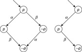
Suppose that actions α and β of the state space depicted in Figure 10.17 are independent and that α is invisible with respect to the set of propositions p. Suppose further that we want to search for a goal ¬p, where p is an atomic proposition. With these assumptions the reduced state space for the example is stuttering equivalent to the full one. The shortest path that violates the invariant in the reduced state space consists of actions α and β, which has a length of 2. In the full one, the initial path with action β is the shortest path to a goal state, such that the corresponding solution path has a length of 1.
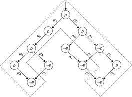
The problem can be partially avoided by postprocessing the solution. The intuitive idea is to ignore those actions that are independent from the action that directly led to the goal state, since they are not relevant. To get a valid solution path it is also necessary to require that the ignored actions cannot enable actions that occur after them in the original solution. The approach may be able to shorten the established solution path, but the resulting solution may not be optimal. Figure 10.18 depicts an example of a full state space and a possible reduction. As in the example in Figure 10.17, a goal state is one in which proposition p does not hold. Suppose that the following pairs of actions are independent—(α3, α4), (α6, α7), and (α6, α8)—and that only α6 and α4 are visible and negate the value of the proposition p. Then, the path formed by actions α1, α2, α3, and α4 can be established as the shortest path in the reduced state space denoted by the dashed region. Applying the approach can result in the solution path α1α2α4, which has a length of 3. This is possible since α3 is invisible, independent from α4 and cannot enable α4. On the other hand, the optimal solution in the full state space is shorter: α5α6.
10.3. Summary
In this chapter, we studied pruning to make searches more efficient. Pruning means to ignore parts of the search tree (and thus reduce the branching factor) to save runtime and memory. This can be tricky since we would like the search to find a shortest path from the start state to any goal state (admissible pruning) or at least some path from the start state to a goal state (solution preserving pruning) if one exists. Also, pruning itself requires runtime and memory, and thus we need to ensure that these costs are outweighed by the corresponding savings. Pruning often exploits regularities in the state space, knowledge of which can be supplied by an expert or learned automatically. The learning can happen either before the search (static pruning), often in similar but smaller state spaces than the ones to be searched, or during the search (dynamic pruning). If it is done during the search, it can be done as part of finding a path from the start state to a goal state or as part of a two-level architecture where the top-level search finds a path from the start state to a goal state and lower-level searches acquire additional pruning knowledge.
We discussed the following admissible pruning strategies:
• Substring pruning prunes action sequences (called duplicates) that result in the same state as at least one no-more-expensive nonpruned action sequence (called the shortcut). Thus, this pruning strategy is an alternative to avoiding the regeneration of already generated states for search algorithms that do not store all previously generated states in memory, such as IDA*, and thus cannot easily detect duplicate states. We discussed two static ways of finding duplicate action sequences, namely by a breadth-first search that finds action sequences that result in the same state when executed in the same state and by detecting action sequences that result in the same state in which they are executed (cycles). For example, URDL is a cycle in an empty Gridworld, implying that UR is a duplicate action sequence of RU (the inverse of DL) and ULD is a duplicate action sequence of R (the inverse of L). We also discussed a dynamic way of finding duplicate action sequences, namely during an A* search. To be able to detect duplicate action sequences efficiently, we can encode them as finite-state machines, for example, using the Aho-Corasick algorithm. We used the Eight-Puzzle to illustrate substring pruning.
• Dead-end pruning prunes states from which no goal state can be reached. A state can be labeled a dead-end if all successor states of it are dead-ends or by showing that one simplification (called decomposition) of it is a dead-end. We discussed a static way of finding dead-ends (called bootstrapping), namely using penalty tables. Penalty tables are a way of learning and storing more informed heuristics, and an infinite heuristic indicates a dead-end. We also discussed a dynamic way of finding duplicate action sequences, namely during an A* search (resulting in abstraction decomposition A*). We used Sokoban to illustrate dead-end pruning.
• Symmetry reduction prunes action sequences that are similar (symmetric) to a same-cost, nonpruned action sequence. We discussed a dynamic way of symmetry reduction that exploits transpositions of state variables and uses some precompiled knowledge of symmetry between variables in the goal state.
We discussed the following nonadmissible pruning strategies:
• Macro problem solving prunes actions in favor of a few action sequences (called macros), which not only decreases the branching factor but also the search depth. We discussed a static way of macro learning for the Eight-Puzzle where the macros bring one tile after the other into place without disturbing the tiles brought into place already.
• Relevance cuts prune actions in a state that are considered unimportant because they do not contribute to the subgoal currently pursued. Actions that do not influence each other are called distant actions. Relevance cuts can, for example, prune an action if more than a certain number of distant actions have been executed recently (because the action then does not contribute to the subgoal pursued by the recently executed actions) or if the action is distant to the last action but not a certain number of actions that have been executed recently (because the action then does not contribute to the subgoal pursued by the last action that already switched the subgoal pursued by the actions executed before). We used Sokoban to illustrate relevance cuts.
• Finally, partial order reduction prunes action sequences that result in the same state as at least one nonpruned action sequence. Different from substring pruning, the nonpruned action sequence can be more expensive than the pruned action sequence. The nonpruned actions are called ample actions. We discussed a way of determining the ample actions, utilizing properties of the actions, such as their independence and invisibility, so that action sequences from the start to the goal are not searched only if they are stuttering equivalent to an action sequence from the start to the goal that is searched. We discussed ways of postprocessing the found action sequence to make it shorter, even though neither the partial order–reduced sequence nor the postprocessed one can be guaranteed to be shortest.
Table 10.4 compares the state space pruning approaches. The strategies are classified along the criteria whether or not they are admissible (i.e., preserve optimal solutions in optimal solvers) or incremental (i.e., allow detection and processing of pruning information during the search). Pruning rules are hard criteria and can be seen as assigning a heuristic estimate ∞ to the search. Some rules extend to refinements to the admissible search heuristic, lower bound. The classification is not fixed; refer to the presentation in the text. Depending on weakening (strengthening) assumptions for the pruning scenario, admissible pruning techniques may become inadmissible (and vice versa). We also provide some time efficiencies for storing and applying the pruning, which, of course, depend on the implementation of the according data structure and neglect some subtleties provided in the text. For substring pruning we assume the Aho-Corasick automaton (IDA*) or suffix trees (IDLA*). For dead-end pruning and pattern search, a storage structure based on partial states is needed. Symmetries can either be provided by the domain experts or inferred by the system (action planning). For the sake of a concise notation, in action planning and Sokoban we assumed a unary Boolean encoding of the set of atoms (squares) to form the state vector.
10.4. Exercises
10.1 Assume that we have found a pruning pair (d, c) according to its definition. Show that pruning substrings d from search tree paths p is admissible.
10.2 Determine all duplicate/shortcut string pairs for the (n2 − 1)-Puzzle of accumulated length 12, by a hash lookup in depth 6 of a breadth-first search enumeration of the search space. Use the lexicographic ordering on the characters to differentiate between duplicate and shortcuts. Build the corresponding finite-state machine that accepts the duplicate strings.
10.3 Complex dead-end positions in Sokoban are frequent.
1. Find a dead-end pattern u in Sokoban with more than eight balls.
2. Show how pattern search determines the value ∞ for u.
3. Display the tree structure for learning the dead-end position with root u.
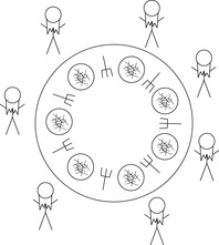
10.4 In Dijkstra's Dining Philosophers problem (see Fig. 10.19) n philosophers sit around a table to have lunch. There are n plates, one for each philosopher, and n forks located to the left and to the right of each plate. Since two forks are required to eat the spaghetti on the plates, not all philosophers can eat at a time. Moreover, no communication except taking and releasing the forks is allowed. The task is to devise a local strategy for each philosopher that lets all philosophers eventually eat. The simplest solution, to access the left fork followed by the right one, has an obvious problem. If all philosophers wait for the second fork to be released there is no possible progress: a dead-end has occurred.
10.5 For computing symmetries in a logistic planning domain with 10 cities, 10 trucks, 5 airplanes, and 15 packages, determine
1. The number of symmetries that respect the type information.
2. The number of variable symmetries that respect variable types.
10.6 A relevance analysis precomputes a matrix D of influence numbers. The larger the influence number, the smaller the influence. One suggestion for calculating D is as follows. Each square on the path between start and goal squares adds 2 for each alternative route for the ball and 1 for each alternative route for a man. Every square that is part of an optimal path will only add half that amount. If the connection from the previous square on the path to the current square can be taken by a ball only 1 is added, else 2. If the previous square is in a tunnel, value 0 is added regardless of all other properties.
1. Compute a relevance matrix D for the problem in Figure 10.20.
2 Run a shortest path algorithm to find the largest influence between every two squares.

10.7 Provide macros for the (3-blocks) Blocksworld problem.
1. Display the state space problem graph based on the actions stack, pickup, putdown, and unstack.
2. Form all three-step macros, and establish a macro solution in which a is on top of b and b is on top of c starting from the configuration, where all blocks are on the table.
1. Define a state vector representation for Rubik's Cube that allows you to build a macro table. How large is your table?
2. There are different solution strategies for incrementally solving the Cube available on the Internet. Construct a macro table based on the 18 basic twist actions.
3. Construct a macro table automatically by writing a computer program searching for one (shortest) macro for each table entry.
10.9 Macro problem solving is only possible if the problem can be serialized; that is, if finding the overall goal can be decomposed into an incremental goal agenda.
1 Give a formal characterization of serialization based on a state vector representation (v1, …, vk) of the problem that is needed for macro problem solving.
2 Provide an example of a domain that is not serializable.
10.10 Show the necessity of condition C3 in partial order reduction! Consider the original state space of Figure 10.21 (left). Proposition p is assumed to be contained in the goal description. Starting with S1 we select ample(S1) = α1, for S2 we select ample(S2) = α2, and for S3 we select ample(S3) = α3.
1. Explain that β is visible.
2. Show that the three ample sets satisfy C0, C1, and C2.
3. Illustrate that the reduced state graph in Figure 10.21 (right) does not contain any sequence, where p is changed from true to false.
4 Show that each state along the cycle has deferred β to a possible future state.
10.11 Prove the correctness of partial order reduction according to condition C3duplicate for depth-first, breadth-first, best-first, and A*-like search schemes. Show that for each node u the following is true: When the search of a general search algorithm terminates, each action α ∈ enabled(u) has been selected either in ample(u) or in a node v such that v has been expanded after u.
10.5. Bibliographic Notes
The pattern matching approach of Aho and Corasick (1975) is a generalization of the algorithm of Knuth, Morris, and Prat (1977). The latter has been extended to include character wild cards. Finite-state machine pruning based on Aho and Corasick's approach is best documented in Taylor's PhD thesis (1997). The usability of suffix trees in state space search is due to Edelkamp (1997).
Dead-end pruning in Sokoban has been first suggested by Junghanns and Schaeffer (1998). The presented algorithmic approach on abstraction and decomposition in A* is based on similar findings in Edelkamp (2003a). Pattern search has been introduced by Junghanns and Schaeffer (1998). The idea shares similarities with Partition Search by Ginsberg (1996), where the entries of a hash table are generalized to hold information about sets of problem states. Pattern searches are a conflict-driven top-down proof of correctness, whereas the Method of Analogies by Adelson-Velskiy, Arlazarov, and Donskoy (2003) is a bottom-up heuristic approximation.
State space reduction based on symmetry relations is frequently met in state space search literature. Symmetries are referred to in the context of pattern databases in Culberson and Schaeffer (1998). Action planning symmetries have been intensively studied by Fox and Long (1999), Rintanen (2003) and Edelkamp (2003c). In the area of model checking, symmetry reduction is also fundamental. A combination of symmetry reduction and directed search for the design of admissible symmetric estimates has been given by Lluch-Lafuente (2003b).
The macro problem solver by Korf (1985b) refers to his PhD thesis work. There is much work on the formation of macros in machine learning (Langley, 1996). Strips, nowadays used as an acronym for a basic specification language in action planning, actually refers to a planning system by Fikes and Nilsson (1971) that is based on macros. An application of so-called partial order macros to scale up action planners has been provided by Botea, Müller, and Schaeffer (2005).
Relevance cuts have been proposed and theoretically studied (Junghanns and Schaeffer, 2001) in the context of Sokoban. In two-player search, a number of meta-level reasonings such as null-move search (Goetsch and Campbell, 1990) and futility cut-offs (Schaeffer, 1986) are known.
Two main families of partial order techniques exist. The first one is based on net unfoldings as described by Bornot, Morin, Niebert, and Zennou (2002) and the second is based on the so-called diamond properties. We have focused on the latter, which are called partial order reduction techniques. Several partial order reduction approaches have been proposed, namely those based on stubborn sets by Valmari (1991), persistent sets by Godefroid (1991) and ample sets by Peled (1996). Although they differ in details, they are based on similar ideas. Due to its popularity, we mainly followed the ample sets approach. Nonetheless, most of the reasoning presented in this chapter can be adjusted to any of the other approaches. For an extended description of partial order reduction methods we refer to Peled (1998).
..................Content has been hidden....................
You can't read the all page of ebook, please click here login for view all page.