
Chapter 17. Vehicle Navigation
This chapter gives a general introduction to state space search problems in routing applications. Map matching and various speedup techniques are discussed.
Keywords: vehicle navigation, route guidance, digital map, positioning system, map matching, geocoding, routing algorithm, route planning, time-dependent routing, stochastic routing, cutting corners, container pruning, local A*
Navigation is a ubiquitous need to satisfy today's mobility requirements. Current navigation systems assist almost any kind of motion in the physical world including sailing, flying, hiking, driving, and cycling. This success in the mass market has been largely fueled by the advent of the GLOBAL POSITIONING SYSTEM (GPS), which provides a fast, accurate, and cost-efficient way to determine one's geographical position anywhere on the Earth. GPS is most useful in combination with a digital map; map matching can provide the user with the information of where he or she is located with regard to it. However, for use in a vehicle, it is not only desirable to know the current position, but also to obtain directions of how to get from the current position to a (possibly unknown) target. To solve this problem, route finding has become a major application area for heuristic search algorithms.
In this chapter, we briefly review the interplay of search algorithms and other components of navigation systems, and we discuss particular algorithmic challenges arising in this field.
17.1. Components of Route Guidance Systems
Let us first give a brief overview of the different components of a navigation system. Apart from the routing algorithm, relevant aspects include the generation and processing of suitable digital maps, positioning, map matching, geocoding, and user interaction. The next sections discuss these topics in turn.
17.1.1. Generation and Preprocessing of Digital Maps
Digital maps are usually represented as graphs, where the nodes represent intersections and the edges are unbroken road segments that connect the intersections. Nodes are associated with a geographical location. Between intersections intermediate nodes of degree 2 (so-called shape points ) approximate a road's geometry.
Each segment has a unique identifier and additional associated attributes, such as the name, the road type (e.g., highway, on-/off-ramp, city street), speed information, address ranges, and the like. Generally, no information about the number of lanes is provided. The straightforward representation for a two-way road is by means of a single undirected segment. However, for navigation purposes a representation that breaks them up into two unidirectional links of opposite direction is often more convenient.
Today's commercially available digital maps have achieved an accuracy in the range of a few to a few tens of meters, as well as a coverage for all the major highway road network and urban regions in the industrialized world. They are produced based on a variety of sources: digitization of legacy (paper) maps, aerial photographs, and data collection by specialized field personnel with proprietary equipment, such as optical surveying instruments and high-precision GPS receivers. Maps can be digitized by hand, tracing each map's lines with a cursor, or automatically with scanners. Since maps are bound to change continually over time, updates have to be supplied on a regular basis, typically once or twice a year.
Besides navigation, the combination of enhanced digital roadmaps and precise positioning systems enables a much wider range of novel in-car applications that improve safety and convenience, such as curve speed warning, lane departure detection, predictive cruise control for fuel savings, and more. However, for such applications current commercial maps still lack some necessary features and accuracy, such as accurate altitude, lane structure, and intersection geometry. A number of national and international research efforts are currently under way to investigate the potential of these technologies, like the U.S. Department of Transportation project EDMap and its European Union counterpart NextMap, which are similar in scope. The objective of EDMap was to develop and evaluate a range of digital map database enhancements that might enable or improve the performance of driver assistance systems under development or consideration by automakers. The project partners included several automotive manufacturers and map suppliers.
Alternative approaches to the traditional labor- and equipment-intensive process of map generation have been researched, and prototypical systems have been developed. One such proposition is statistical in spirit: It is based on a large quantity of possibly noisy data from GPS traces for a fleet of vehicles, as opposed to a small number of highly accurate points obtained from surveying methods. It is assumed that the input probe data are obtained from vehicles that go about their usual business unrelated to the task of map construction, possibly piggybacking on other applications based on positioning systems. The data are (semi-)automatically processed in different stages. After data cleanup and outlier removal, traces from different cars are split into sections that belong to the same segment and pooled together, based on an initial inaccurate map, or unsupervised road clustering. Then, each segment geometry is refined using spine fitting. The histogram of distances of GPS points to the road centerline is used to determine the number and position of lanes; finally, observed lane transitions at intersections help to connect the lanes to intersection models.
In a separate project, techniques for offline and online generation of sparse maps has been developed, tailored to use in small, portable devices. The map is based on a collection of entire routes. Intersection points are identified, and segments comprise not individual roads, but subsections of traces not intersecting other traces. Heuristic search methods are needed to estimate if traces represent the same road.
Regardless of the way a digital map has been generated, for navigation purposes it has to be brought in efficiently manageable data structures. The requirements of a routing component are often different from the map display and map matching component, and need a separate representation. For routing, we do not need to explicitly store shape points, only the combined distance and travel times of the line segments between two intersections is relevant for routing. Still, many intersection nodes of degree 2 remain. These nodes can be eliminated by merging the adjacent edges through adding their distance and travel time values.
To find roads that are close to a given location, we cannot afford to sift extensively through large networks. Appropriate spatial data structures access methods (e.g., R-tree, CCAM) have been developed that allow fast location-based retrieval, such as range queries. Recently, some general-purpose databases have begun incorporating spatial access methods.
17.1.2. Positioning Systems
Positioning system is a general term to identify and record the location of an object on the Earth's surface. There are three types of positioning systems commonly in use: standalone, satellite-based, and terrestrial radio-based.
Stand-alone Positioning Systems
Dead reckoning (DR) is the typical standalone technique that sailors commonly used in earlier times before the development of satellite navigation. To determine the current position, DR incrementally integrates the distance traveled and the direction of travel relative to a known start location. A ship's direction used to be determined by magnetic compass, and the distance traveled was computed by the time of travel and the speed of the vehicle (posing the technical challenge of building mechanical clocks that work with high accuracy in an environment of rough motions and changing climates). In modern land-based navigation, however, various sensor devices can be used, such as wheel rotation counters, gyroscopes, and inertial measurement units (IMUs). A common drawback of dead reckoning is that the estimation errors increase with the distance to the known initial position, so that frequent updates with a fixed position are necessary.
Satellite-Based Positioning Systems
With a GPS receiver, users anywhere on the surface of the Earth (or in space around the Earth) can determine their geographic position in latitude (north–south, ascending from the equator), longitude (east–west), and elevation. Latitude and longitude are usually given in units of degrees (sometimes delineated to degrees, minutes, and seconds); elevation is usually given in distance units above a reference such as mean sea level or the geoid, which is a model of the shape of the Earth.
The Global Positioning System was originally designed by the United States Department of Defense for military use. It comprises 24 satellites orbiting at about 12,500 miles above the Earth's surface. The satellites circle the Earth about twice in a 24-hour period. Each GPS satellite transmits radio signals that can be used to compute a position. These signals are currently transmitted on two different radio frequencies, called L1 and L2. The civilian access code is transmitted on L1 and is freely available to any user, but the precise code is transmitted on both frequencies, and can be used only by the U.S. military.
To calculate a position, a GPS receiver uses a principle called triangulation (to be precise: trilateration ), a method for determining a position based on the distance from other points or objects that have known locations.
The satellite's radio signals carry two key pieces of information—its position and velocity—and a digital timing signal based on an accurate atomic clock on board the satellite. GPS receivers compare this timing information to timing information generated by a clock within the receiver itself to determine the time it took the radio signal to travel from the satellite to the receiver (and hence its distance, taking into account the speed of light).
Since each satellite measurement constrains the location to lie on a sphere around it, the information of three satellites leaves only two possible positions, one of which can generally be ruled out for not lying on the Earth's surface. So, although in principle three satellites are sufficient for localization, in practice another one is needed to compensate for inaccuracies in the receiver's quartz clock.
Obviously with such a sophisticated system, many things can cause errors in the positional computation and limit the accuracy of measurement. Apart from clock errors, major noise sources are:
• Atmospheric interference: The signal is deflected by the ionosphere, and has to travel a longer distance, particularly for satellites that stand low over the horizon.
• Multipath: The signal is reflected at nearby buildings, trees, and such, so that the receiver has to distinguish between the original signal and its echo.
• Due to the various external gravitational influences, the satellite's orbit can deviate from the theoretical prediction.
To achieve higher position accuracy, most GPS receivers utilize what is called differential GPS (DGPS). A DGPS receiver utilizes information from one or more stationary base-station GPS receivers. The base-station GPS receiver calculates a position from the satellite signals, and its difference from the accurately known real position. Under the valid assumption that nearby locations experience a similar error (e.g., due to atmospheric noise), the difference is broadcast to the mobile receivers, who add it to their computed position. Publicly available differential correction sources can be classified as either local area or wide area broadcasts. Local area differential corrections are usually broadcast from land-based radio towers and are calculated from information collected by a single base station. The most common local area differential correction source is a free service maintained by the U.S. Coast Guard. Wide area differential corrections are broadcast from geostationary satellites and are based on a network of GPS base stations spread throughout the intended coverage area. A common source for different corrections used by many low-cost GPS receivers is the Wide Area Augmentation System (WAAS). It is broadcast on the same radio frequency as the GPS signals; therefore, the receivers can conveniently obtain it using the same antenna.
The European Galileo program will build a civilian global navigation satellite system that is interoperable with GPS and the Russian GLONASS. By offering dual frequencies as standard, however, Galileo will deliver real-time positioning accuracy down to the meter range, which is unprecedented for a publicly available system. It is planned to reach full operational capability with a total of 30 satellites.
Terrestrial Radio-Based Positioning Systems
Apart from satellite-based navigation, terrestrial radio-based positioning systems have been designed for specific applications (e.g., offshore navigation). They commonly employ direction or angle of arrival (AOA), absolute timing or time of arrival (TOA), and differential time of arrival (TDOA) techniques to determine the position of a vehicle. For example, LORAN-C consists of a number of base stations at known locations that keep sending a synchronized signal. By noting the time difference between the signals received from two different stations, the position can be constrained to a hyperbola; exact location requires a second pair of base stations.
Indoor navigation systems generally use infrared and short-range radios, or radio frequency identification (RFID). The mobile networking community uses a technique known as cell identification (Cell-ID).
Hybrid Positioning Systems
We have seen that dead reckoning can maintain the position independently of the availability of external sources, however, it needs regular fixes with known positions or the error will increase steeply with the distance traveled. On the other hand, satellite-based or terrestrial positioning systems can provide an accurate position, but are not available everywhere or all the time (e.g., GPS needs a clear view of the sky, rendering it unreliable in tunnels or urban canyons). Therefore, many practically deployed positioning systems employ a combination of fixed positioning and dead reckoning. Most factory-installed navigation systems use a combination of (D)GPS with wheel rotation counters, gyroscopes, and steering wheel sensors. A universal, principled way of integrating several noisy sensors into a consistent estimate is the Kalman filter. To use the Kalman filter to estimate the internal state of a process given only a sequence of noisy observations, we must supply a time-dependent model of the process. In our case, it must be specified how variables like speed and acceleration at a discrete time instant t evolve from a given state at time t − 1. In addition, we have to define how the observed outputs depend on the system's state, and how the controls affect it. Then, the process can be essentially modeled as a Markov chain built on linear operators perturbed by Gaussian noise.
Factory-installed vehicle navigation systems can offer a higher positional accuracy than handheld devices due to the integration of built-in sensors. Due to the big gap in cost, however, the latter ones are becoming more and more popular, especially in Europe.
17.1.3. Map Matching
Map matching means associating a position given as a longitude/latitude pair with the most probable location with regard to a map. With perfect knowledge of the location and flawless maps, this would be a trivial step. However, GPS positions might sometimes deviate from the true position by tens to hundreds of meters; and in addition, digital maps contain inaccuracies in the geometry of roads, spurious or missing segments. Moreover, roads are usually represented as lines, and intersections simplified as points where segments meet. Real roads, however, particularly multilane highways, have a nonnegligible width; real intersections also have a considerable extent, and can comprise turn lanes.
Geometric techniques utilize only the estimated location(s) and the road segments. We can distinguish between point-to-point matching, point-to-curve matching, and curve-to-curve matching. In point-to-point matching (see Fig. 17.1), the objective is to find the closest node ni to the measured position p(e.g., the location predicted by GPS). Generally, the Euclidean distance is used to find the distance between p and ni. The number of nodes ni is quite large in a road network; however, this number can be reduced using a range query with a suitable window size and the appropriate spatial access method (e.g., R-tree, CCAM). Point-to-point matching gives inaccurate results when we are in the middle of a segment, far away from intersections.
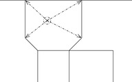 |
| Figure 17.1 |
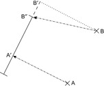
In point-to-curve matching (see Fig. 17.2), the objective is to find the closest curve from the measured point. Since most common map segments are represented as a sequence of line segments (a so-called polyline ), we find the minimum distance between p and any point on some line segments li. The procedure consists of projecting a point on a line segment (see Fig. 17.3). Generally, we can first retrieve a set of candidate segments with a range query centered on p. Then, each line segment of each road is tested in turn.
 |
| Figure 17.2 |
To improve efficiency, a bounding box can be associated with each segment. Formally, theaxis-parallel bounding boxfor a set of coordinates P is defined as the smallest enclosing rectangle [x1, x2] × [y1, y2] for P; that is,  ,
,  ,
,  ,
,  . Then, irrelevant segments can be excluded with little effort by computing the distance of p to the bounding box first; we continue with the actual sequence of projections only if it is sufficiently small (i.e, smaller than the best line segment found so far). Apart from the location of a vehicle, it is also often worthwhile to take into account theheading(direction of travel) of the vehicle for disambiguation between two close segments running in different directions, for example, in the vicinity of intersections.
Still, point-to-curve matching has limitations. For example, a frequently observed problem in current navigation systems is that a vehicle on a freeway is mapped to an exit ramp, which runs almost parallel (or vice versa). Due to map inaccuracy and the width of lanes, the closest line segment is indeed on the wrong street. In this case, taking into account only proximity and heading of the current position is not enough.
A more accurate geometric method, curve-to-curve matching (see Fig. 17.4), uses not only the current point pn, but an entire (segment of the) polyline of historical positions p0, p1,…,pn, the so-called trace of the vehicle, simultaneously to find the most probable line segment. The knowledge of a vehicle's previous segment constrains the subsequent segment to one of the outgoing edges of its head node. Since alternative candidate routes have to be maintained in parallel and simultaneously extended, it turns out that heuristic search algorithms, most notably A*, provide the best map matching results. Each state in the search consists of a match between a position pi and a line segment, and its successors are all matches of pi+1 that are consistent with the map; that is, they are matched either to the same segment, or to any segment that is connected to it in the direction of travel. As a cost measure, we can apply projected point distance, heading difference, or a weighted combination of the two.
 |
| Figure 17.4 |
Often, digital maps have a higher relative accuracy than absolute accuracy; that means that the distance error between adjacent shape points is much smaller than the distance between the latitude/longitude position of a shape point and its ground truth. In other words, the map can be locally shifted. An effective way of compensating for these types of inaccuracies is to use a cost function in the A* algorithm that penalizes discrepancies between the driven distance, as estimated from the vehicle trace, and the distance between the matching start and end points according to the digital map.
In summary, a search algorithm (heuristic or not) performing curve-to-curve matching can correct for GPS and map inaccuracies much more effectively than simple point-to-curve matching. In exchange, considerably more computation effort is involved. Therefore, it is used where accuracy is of primary concern, such as in automatic lane keeping or map generation (see the previous section); if rapid response is more important than occasional errors, such as in most navigation systems, point-to-curve matching is employed.
17.1.4. Geocoding and Reverse Geocoding
Geocoding is the term used for determining a location along a measured network; typically this means transforming a textual description, such as a street address, into a location. Conversely, reverse geocoding maps a given position into a normalized description of a feature location. Reverse geocoding, therefore, includes map matching, to be discussed in the next section.
Often, maps do not contain information about individual buildings, but address ranges for street segments. Geocoding then applies interpolation: If the address range of a street segment spans the address being geocoded, a point location will be created where that address should be. For instance, 197 will be located 97% of the way from the 100 end of the 100–199 block of Main Street (to be precise: 97 / 99 ⋅ 100 = 97.97%). Another limitation is the network data used—if there are inaccuracies in the street network, the geocoding process will produce unexpected results.
17.1.5. User Interface
The market acceptance of commercial routing systems depends largely not only on the quality of the map data and the speed and accuracy of the search algorithm, but also on the interaction with the user. This starts with the convenience of entering start and target destinations, which involves geocoding (see Sec. 17.1.4), but also search capabilities and tolerance against variations of address format, slight spelling errors, and so on. Speech recognition plays an important role for in-vehicle systems.
After a route has been found, the system provides the driver with spoken and/or visual advice to guide him to his destination. If available, a graphical map display must look appealing, and find the right scale and detail of presentation. For offline navigation, a textual route description is generated; in on-board systems, the position of the car is used in combination with the current route to determine the necessary advice and the timing of giving advice. Usually, the driver first receives a warning that he should prepare to make a certain turn ahead of time so that he can actually make the necessary preparations, such as changing lanes and slowing down. Then the actual advice is given. While the driver is progressing toward his destination, the car navigation system monitors the progress of the car by comparing the current position and the presented route. Of course, not all drivers (correctly) follow all instructions. If the car is not positioned on the current route for a certain amount of time, then the system concludes the driver has deviated from his route, and a new route needs to be planned from the position of the car to the destination.
17.2. Routing Algorithms
The route planning algorithm implemented in most car navigation systems is an approximation algorithm based on A*. The problem can become challenging due to the large size of maps that have to be stored (it is an example of a graph that has to be stored explicitly ). Moreover, constraints on the available computation time of the algorithm are often very tight due to real-time operation. As we will see, to speed up computation, some shortcut heuristics are applied that sometimes result in nonoptimal solutions. Often, at the start an initial route is presented to the driver. As the driver progresses along the proposed route, the system can recalculate the route to find successive improvements.
Car navigation systems usually provide the option to choose among several different optimization criteria. In general, the driver can choose between planning a fastest route, a shortest route, and a route giving preference or penalties to freeways. Also, options to avoid toll roads or ferries may be available. In the future, we expect to see an increase in the personalization of planned routes, by an increasing adaptation of the used cost functions to the preferences of the individual driver.
Another aspect of the quality of routes in real-life situations concerns traffic conditions. Information can be static (e.g., average rush-hour and off-peak speeds) or be received online wirelessly (e.g., by radio (RDS) or cell phone). Taking traffic information into account for route planning is a major challenge of a navigation system.
Another real-life requirement that is often overlooked when applying heuristic search to a road network is the existence of traffic rules. At a particular intersection, the driver, for example, may not be allowed to make a right turn. Traffic rules can be modeled by a cost function on pairs of adjacent edges. If a traffic rule exists that forbids the driver to go from one road segment to another, then an infinite cost is associated with that pair of adjacent edges. In extension, this formalism also allows us to flexibly encode travel time estimates for intersections (on average, left turns take more time than right turns or straight continuations). The cost of a path P with edges e0,…,en is defined as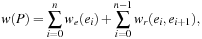 where we is the edge cost and wr is the cost associated with turning from ei to ei+1.
In the straightforward formalization of the state space, intersections are identified with nodes, and road segments between them as edges. However, this is no longer feasible in the presence of turn restrictions. Because an optimum route may contain a node more than once, the standard A* algorithm cannot be used to determine the optimum route. However, an optimum route does not contain an edge more than once. To plan optimum routes in a graph with rules, a modified A* algorithm can be used that evaluates edges instead of nodes. The g-value of an edge e reflects the path cost from the start node up to the head node of e. Additionally, a value gn associated with each node n is maintained, which keeps track of the minimum of all g-values of edges ending in n.
17.2.1. Heuristics for Route Planning
When trying to find a shortest route, the edge costs are equal to the length of the edge. The (modified) A* algorithm can use an h -value based on the Euclidean distance, or bee line, from the geographical location L (u) associated with the node u to the location of the destination t. The Euclidean distance between Cartesian coordinates p1 = (x1, y1) and p2 = (y2, x2) is defined as where
where  denotes the so-called L2-norm. The heuristic h (u) = d (L (u), L (t)) is a lower bound, since the shortest way to the goal must be at least as long as the air distance. It is also consistent, since for adjacent nodes u and v,
 by the triangle inequality of the Euclidean plane. Therefore, no reopening is needed in the algorithm.
As for the fastest route, it is common to estimate travel time based on road classes. Every segment of the road network has been assigned a certain road class. This road class can be used to indicate the importance of a road: the higher the road class number the less important the road. For example, edges with road class 0 are mainly freeways, and edges with road class 1 are mainly highways. An average speed is associated with each road class, and the cost of an edge is determined as its length, divided by this speed. The Euclidean distance divided by the overall maximum speed vmax can be used as a h -value to plan fastest routes.
Many route planning systems allow the user to prefer a combination between the fastest route and the shortest route. We can express this using a preference parameter τ that determines the relative weights of a linear combination of the two. We define hτ as the heuristic estimate for a node u in this extended model as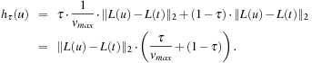 Since τ and vmax are constant for the entire graph and
  never overestimates the actual edge cost, hτ never overestimates the actual path cost; that is, it is admissible.
17.2.2. Time-Dependent Routing
Certain properties of a road network change over time. Roads may be closed during specific time periods. For example, a road can be closed for construction work during several hours or days. Particularly during rush hours, the driving time of a route is typically longer. To take this into account, the basic model has been extended to handle time-dependent costs. The weight functions we and wr accept an additional argument, representing time. We also define analogous functions te (e, t) and tr (e1, e2, t) that denote the time needed to pass an edge and for turning between edges at time t, respectively (for the case of the shortest route, te = we and tr = wr). This formalism also allows, for example, for modeling phases of stoplights. The cost of a path P = (e0,…,en) at departure time t0 is calculated as where
where  denotes the arrival time at the head node of edge ei+1.
In this formalism, however, some assignments of time-dependent costs lead to complications. As an extreme case, suppose that for a ferry that operates only during certain times, we assign a weight of infinity outside that interval. Then a vehicle starting at a certain time might not find a possible route with finite weight at all, whereas it can be possible for a later departure. It can be optimal to delay the arrival at a node u if the cost of the time-route from node u to the destination decreases more than the cost of the time-route from the starting point to node u increases by delaying the arrival. This means that cycles or large detours can be actually beneficial. It has been shown that finding an optimal route for the general case of time-dependent weights is NP-hard.
To apply (a variant of) Dijkstra's algorithm or the A* algorithm, we have to ensure the precondition of Bellman's principle of optimality; that is, that every partial time-route of an optimum time-route is itself an optimum time-route (see Sec. 2.1.3). Let h * (e, t0) denote the minimum travel time to get to the goal, starting at time t0 from the tail node of edge e. Then the road graph is called time-consistent if for all times t1 ≤ t2, and every pair of adjacent edges e1 and e2, we have Roughly speaking, this condition states that leaving a node later can perhaps reduce the duration of traversing an edge, but it cannot decrease the arrival time at the goal. Time consistency of a road graph implies that the Bellman condition holds.
To show time consistency, it turns out that we do not have to explicitly inspect the routes between all pairs of start and destination nodes; instead, it is sufficient to check every pair of adjacent edges. More precisely, we have to verify the condition that for all times t1 ≤ t2 and every pair of adjacent edges e1 and e2, we have Then time consistency of the road graph follows from a straightforward induction on the number of edges in the solution path.
The model can be generalized to the case that we are trying to minimize a cost measure different from travel time, for example, distance. Then, besides time consistency, the feasibility of the search algorithm requires cost consistency. A road graph is called cost consistent if for every minimum-cost time-route (e1,…,en) departing at time t0 from node s to node d, the partial route (e1,…,ei) departing at t0 is also an optimal route from s to ei. In addition, if there are two minimum-cost time-routes from node s to edge ei with identical cost, then the time-route (e1,…,ei) is the one with the earliest arrival time at the head node of ei. Unlike for time consistency, unfortunately, there is no easy way of verifying cost consistency without planning the routes between all pairs of nodes.
Under the aforementioned properties of time and cost consistency, the Bellman equation holds, and we can apply the A* algorithm for route finding. The only modification we have to make is to keep track of the arrival time at the end node of each edge, and to use this arrival time to determine the (time-dependent) cost of its adjacent edges.
17.2.3. Stochastic Time-Dependent Routing
The time-dependent costs from the last section can be used to model a variety of delays in travel time, for example, congestion during rush hours, traffic lights timing, timed speed or turn restrictions, and many more conditions. However, it goes without saying that the exact progress a particular driver will make at a certain time is unknown. In this section, we are concerned with attempts to model the uncertainty of the prediction.
In the most general setting, the cost and driving time of an edge e is a random variable described by a probability density function f (e, t). However, in such a formalism the complexity of calculating the stochastic cost of a route can be tremendous; it involves a detailed computation of all possible combinations of realized travel times for the edges in the route. To see this, consider a trip consisting of only two edges, e1 and e2. The probability that the trip takes k seconds is equal to a very lengthy sum, namely, of the probability that e1 takes 1 second and e2 takes k − 1 seconds, plus the probability that e1 takes 2 seconds and e2 k − 2 seconds, and so on. In the continuous case, we have to form an integral, or more precisely, what is known as a convolution. These operations would be computationally infeasible for practical route planning algorithms.
One way out is to consider only probability density functions of certain parametric forms with nice properties. Thus, it has been proposed that if the travel times are exponentially or Erlang distributed and the travel time profiles have a simple form, then the expected travel time and variance of the travel time of a stochastic time-route can be computed exactly. However, in the following we discuss a different approach.
First, costs and travel times of adjacent edges are assumed to be independent. Turn restrictions are assumed to be certain, and not included in the stochastic modeling. Each edge carries two pieces of information: the mean μ and the standard deviation σ of the cost. The model also includes two factors β and γ to reflect the driver's preferences. The estimated cost of a stochastic path P is defined as  ; in turn, the mean and standard deviation of the weight of the path is computed as
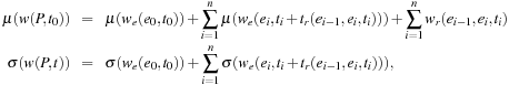 with
with  .
.
Minimizing the estimated cost gives the driver the option to indicate his willingness of taking uncertainty into account when planning a route. For example, for β = 1 a decrease of 10 minutes in the expected travel time and a decrease of 10 minutes in the standard deviation of the travel time are considered equally desirable. For higher values of β, reducing uncertainty becomes more important than reducing the expected travel time. For lower values of β, the situation is exactly the other way around. The factor γ is used to increase the travel time per edge. For γ = 0, the driving time is assumed to be equal to the expected driving time. Setting γ > 0 means the driver is pessimistic about the actual driving time. The larger it is, the more likely the driver will arrive at his destination before the estimated arrival time. This is especially useful for individuals that have an important appointment.
Exactly as in the previous section, we have to ensure the time consistency of the graph to guarantee the Bellman precondition. Taking into account the preference parameters, we have to show for all allowed values for β (or γ), for all times t1 ≤ t2, and all pairs of adjacent edges e1 and e2, that Consequently, the test needs to be performed with the minimum and the maximum allowed value for β.
17.3. Cutting Corners
As mentioned earlier, the requirement of real-time operation, combined with a road graph that can consist of millions of nodes, poses hard time and memory constraints on the search algorithm. Therefore, various pruning schemes have been proposed. Some of the techniques described in Chapter 10 can be applied; in the following, we introduce some methods that are specific to geometric domains.
Nonadmissible pruning reduces computation time or memory requirements by compromising the guarantee of finding an optimal solution. For example, most commercial navigation systems of today incorporate the rationale that when far away from start and goal, the optimal route most likely uses only freeways, highways, and major connections. The system maintains maps on different levels of detail (based on the road class), where the highest one might only contain the highway network, and the lowest level is identical to the entire map. Given a start and destination point, it selects a section of the lowest-level map only within a limited range of both; within larger ranges, it might use an intermediate level, and for the highest distance only the top-level map. This behavior reduces computation time considerably, while still being a good solution in most cases.
Similarly, we know that the Euclidean distance is overly optimistic most of the time. Multiplying it by a small factor, say, 1.1, yields more realistic estimates and can reduce the computation time dramatically, while the solution is often almost identical. This is an instance of nonoptimal A* described in Chapter 6.
The next two sections present two admissible schemes for the reduction of search time.
17.3.1. Geometric Container Pruning
In a domain like route planning, where a multitude of shortest path queries have to be answered on the same problem graph, it is possible to accelerate search by means of pieces of information computed prior to the arrival of the queries. As an extreme case, we could compute and memorize all distances and starting edges for the paths between all pairs of nodes using the Floyd-Warshall (Ch. 2) or Johnson's algorithm; this can reduce the query processing to a mere linear backtracking from target to source. However, the space required for saving this information is O (n2), which is often not feasible because of n being very large. In the next section, we present an approach that reduces the search time in return for more reasonable memory requirements.
Research on annotating a graph by geometric containers to guide a search algorithm has shown significant gains in terms of the number of expanded nodes. The basic idea is to reduce the size of the search space of Dijkstra's algorithm or the A* algorithm by pruning edges that can be safely ignored because they are already known not to lie on a shortest path to the target. The two stages for geometric speedups are as follows:
1. In a preprocessing step, for each edge e = (u, v), store the set of nodes t such that a shortest path from u to t starts with this particular edge e(as opposed to other edges emanating from u).
2. While running Dijkstra's algorithm or A*, do not insert edges into the priority queue of which the stored set does not contain the target.
The problem that arises is that for n nodes in the graph we would need O (n2) space to store this information, which is not practically feasible. Hence, we do not remember the set of possible target nodes explicitly, but approximations of it, so-called geometric containers. For containers with constant space requirement, the overall storage will be in O (n).
A simple example for a container would be an axis-parallel rectangular bounding box around all possible targets. However, this is not the only container class we can think of. Other options are enclosing circles or the convex hull of a set of points P, which is defined as the smallest convex set that contains P. Recall that a set  is called convex if for every two elements
  the line segment between a and b is also completely contained in
  .
.
A container will generally contain nodes that do not belong to the target node set. However, this does not hurt an exploration algorithm in the sense that it still returns the correct result, but increases only the search space. Incorporating this geometric pruning scheme into an exploration algorithm like Dijkstra or A* will retain its completeness and optimality, since all shortest paths from the start to the goal node are preserved.
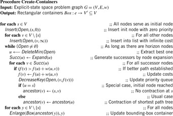
The containers can be computed by Algorithm 17.1 in time O (n2lgn). It essentially solves a sequence of single-source-all-targets problems, for all nodes; a variable ancestor (u) remembers the respective outgoing edge from s used on the shortest path to u. Figure 17.5 shows the result of computing a container for the starting point C and the resulting container for edge (C, D).

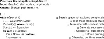
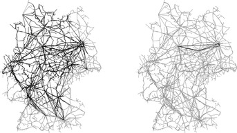
The application of containers in explicit graph search is shown in Algorithm 17.2. While running any optimal exploration algorithm on query (s, t), we do not insert edges into the horizon list that are definitely not part of a shortest path to the target. The time required for the computation of these containers pays off well during the main search. Empirical results show a reduction of 90% to 95% in the number of explored nodes in rail networks of different European countries. Figure 17.6 illustrates the effect of bounding-box pruning in the reduction of traversed edges.
 |
| Figure 17.6 |
It is instructive to compare shortest path pruning to the related approach of pattern database heuristics (see Ch. 15). In the latter case, state-to-goal instead of state-to-state information is stored. Pattern databases are used to refine the search for a fixed goal and varying initial state. In contrast, shortest path pruning uses precomputed shortest path information for a varying initial state and goal state.
17.3.2. Localizing A*
Consider the execution of the A* algorithm on a search space that is slightly larger than the internal memory capacity of the computer, yet not as large to require external search algorithms. We often cannot simply rely on the operating system's virtual memory mechanism for moving pages to and from the disk; the reason is that A* does not respect locality at all; it explores nodes strictly according to the order of f-values, regardless of their neighborhood, and hence jumps back and forth in a spatially unrelated way only for marginal differences in the estimation value.
In the following, we present a heuristic search algorithm to overcome this lack of locality. Local A* is a practical algorithm that takes advantage of the geometric embedding of the search graph. In connection with software paging, it can lead to a significant speedup. The basic idea is to organize the graph structure such that node locality is preserved as much as possible, and to prefer to some degree local expansions over those with globally minimum f-value. As a consequence, the algorithm cannot stop with the first solution found; we adopt the Node-Ordering-A* framework of Chapter 2. However, the overhead in the increased number of expansions can be significantly outweighed by the reduction in the number of page faults.
In the application of the algorithm to route planning we can partition the map according to the two-dimensional physical layout, and store it in a tile-wise fashion. Ideally, the tiles should roughly have a size such that a few of them fit into main memory.
The Open list is represented by a new data structure, called Heap of Heaps (see Fig. 17.7). It consists of a collection of k priority queues H1,…,Hk, one for each page. At any instant, only one of the heaps, Hactive, is designated as being active. One additional priority queue  keeps track of the root nodes of all Hi with i≠active. It is used to quickly find the overall minimum across all of these heaps.
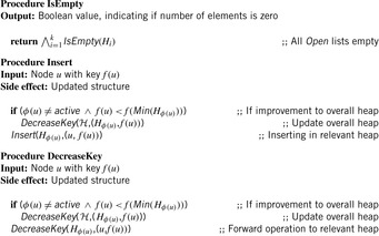
Let node u be mapped to tile ϕ (u). The following priority queue operations are delegated to the member priority queues Hi in the straightforward way. Whenever necessary,  is updated accordingly.
The Insert and DecreaseKey operations (see Alg. 17.3) can affect all heaps. However, the hope is that the number of adjacent pages of the active page is small and that they are already in memory or have to be loaded only once; for example, in route planning, with a rectangular tiling each heap can have at most four neighbor heaps. All other pages and priority queues remain unchanged and thus do not have to reside in main memory. The working set of the algorithm will consist of the active heap and its neighbors for some time, until it shifts attention to another active heap.
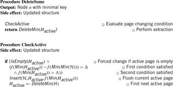
To improve locality of the search, DeleteMin is substituted by a specialized DeleteSome operation that prefers node expansions with respect to the current page. Operation DeleteSome performs DeleteMin on the active heap (see Alg. 17.4).
As the aim is to minimize the number of switches between pages, the algorithm favors the active page by continuing to expand its nodes, although the minimum f-value might already exceed the minimum of all remaining priority queues. There are two control parameters: an activeness bonus Δ and an estimate Λ for the cost of an optimum solution. If the minimum f-value of the active heap is larger than that of the remaining heaps plus the activeness bonus Δ, the algorithm may switch to the priority queue satisfying the minimum root f-value. Thus, Δ discourages page switches by determining the proportion of a page to be explored. As it increases to large values, in the limit each activated page is searched to completion. However, the active page still remains valid, unless Λ is exceeded. The rationale behind this second heuristic is that we can often provide a heuristic for the total least-cost path that is, on the average, more accurate than that obtained from h, but that might be overestimating in some cases.
With this implementation of the priority queue, the algorithm Node-Ordering-A* remains essentially unaltered; the data structure and page handling is transparent to the algorithm. Traditional A* arises as a special case for Δ = 0 and  , where h* (s) denotes the actual minimum cost of a path between the source and a goal node. Optimality is guaranteed, since we leave the heuristic estimates unaffected by the heap prioritizing scheme, and since each node inserted into the Heap of Heaps must eventually be returned by a DeleteMin operation.
The algorithm has been incorporated into a commercially available route planning system. The system covers an area of approximately 800 × 400 km at a high level of detail, and comprises approximately 910,000 nodes (road junctions) linked by 2,500,000 edges (road elements).
For long-distance routes, conventional A* expands the nodes in a spatially uncorrelated way, jumping to a node as far away as some 100 km, but possibly returning to the successor of the previous one in the next step. Therefore, the working set gets extremely large, and the virtual memory management of the operating system leads to excessive paging and is the main burden on the computation time.
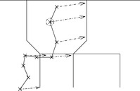
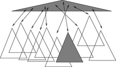
As a remedy, we achieve memory locality of the search algorithm by exploiting the underlying spatial relation of connected nodes. Nodes are geographically sorted according to their coordinates in such a way that neighboring nodes tend to appear close to each other. A page consists of a constant number of successive nodes (together with the outgoing edges) according to this order. Thus, pages in densely populated regions tend to cover a smaller area than those representing rural regions. For not too small sizes, the connectivity within a page will be high, and only a comparably low fraction of road elements cross the boundaries to adjacent pages. Figure 17.8 shows some bounding rectangles of nodes belonging to the same page.
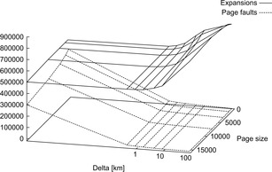
There are three parameters controlling the behavior of the algorithm with respect to secondary memory: the algorithm parameters Δ and Λ and the (software) page size. The latter one should be adjusted so that the active page and its adjacent pages together roughly fit into available main memory. The optimum solution estimate Λ is obtained by calculating the Euclidean distance between the start and the goal and adding a fixed percentage. Figure 17.9 juxtaposes the number of page faults to the number of node expansions for varying page size and Δ. We observe that the rapid decrease of page faults compensates the increase of expansions (note the logarithmic scale). Using an activeness bonus of about 2 km suffices to decrease the value by more than one magnitude for all page sizes. At the same time the number of expanded nodes increases by less than 10%.
17.4. Bibliographic Notes
Astronomical positioning and dead reckoning are nautical techniques thousands of years old. However, though determining latitude had been mastered early on, measuring longitude proved to be extremely harder. Thus, English ships were being wrecked, thousands of lives were lost, and precious cargo wasn't making its scheduled delivery. Competing with the most renowned astronomers of his time, in the early 1700s a simple clockmaker named John Harrison thought that a well-built clock with a dual face would solve the problem. Sobel (1996) has given a fascinating account of Harrison's struggle against enormous obstacles put in his way by an ingrained scientific establishment.
Comprehensive overviews of the components of modern navigation systems and their interaction can be found in Schlott (1997) and Zhao (1997). Advanced vehicle safety applications and the requirements they impose on future digital maps are discussed in the final reports of the EDMap (CAMP Consortium, 2004) and NextMAP (Ertico, 2002) projects. An approach to generate high-precision digital maps from unsupervised GPS traces has been described in Schrödl, Wagstaff, Rogers, Langley, and Wilson (2004). An incremental learning approach for constructing maps based on GPS traces has been proposed by Brüntrup, Edelkamp, Jabbar, and Scholz (2005). GPS route planning on the superposition of traces is proposed by Edelkamp, Jabbar, and Willhalm (2003). It determines intersections of GPS traces efficiently using the sweepline segment intersection algorithm of Bentley and Ottmann (1979), which is one of the first output-sensitive algorithms in computational geometry. The geometric travel planning approach included Voronoi diagrams for query point location search and A* heuristic graph traversal for finding the optimal route. Winter (2002) has discussed modifications to the search algorithm to accommodate turn restrictions in road networks. Our account of time-dependent and stochastic routing is based on the excellent work of Flinsenberg (2004), which should also be consulted for further references on different aspects of routing algorithms. An overview of research concerning real-time vehicle routing problems has been presented by Ghiani, Guerriero, Laporte, and Musmanno (2003).
Shortest path containers have been introduced by Wagner and Willhalm (2003) and been adapted to dynamic edge changes in Wagner, Willhalm, and Zaroliagis (2004). Contraction hierarchies by Geisberger and Schieferdecker (2010) and transit-route routing by Bast, Funke, Sanders, and Schultes (2007) further speed up search. This approach links to initial work by Schulz, Wagner, and Weihe (2000) on shortest path angular sectors. A GPS route planner implementation using shortest path containers in A* has been provided by Edelkamp et al. (2003). Further algorithmic details on dynamic changes to the inferred structures have been discussed in Jabbar (2003). Local A* based on the Heap of Heaps data structure has been proposed by Edelkamp and Schrödl (2000) in the context of a commercial route planning system.
..................Content has been hidden....................
You can't read the all page of ebook, please click here login for view all page.