
Chapter 5. Linear-Space Search
This chapter first studies breadth-first and single-source shortest paths search on logarithmic space. It then introduces and analyzes different aspects of iterative-deepening A* search. The growth of the search tree is estimated and it is shown that heuristics correspond to a relative decrease of the search depth.
Keywords: divide-and-conquer breadth-first search, divide-and-conquer single-source shortest paths, depth-first branch-and-bound, iterative-deepening search, IDA*, search tree prediction, refined threshold determination, recursive best-first search
A* always terminates with an optimal solution and can be applied to solve general state space problems. However, its memory requirements increase rapidly over time. Suppose that 100 bytes are required for storing a state and all its associated information, and that the algorithm generates 100,000 new states every second. This amounts to a space consumption of about 10 megabytes per second. Consequently, main memory of, say, 1 gigabyte is exhausted in less than two minutes. In this chapter, we present search techniques with main memory requirements that scale linear with the search depth. The trade-off is a (sometimes drastic) increase in time.
As a boundary case, we show that it is possible to solve a search problem with logarithmic space. However, the time overhead makes such algorithms only theoretically interesting.
The standard algorithms for linear-space search are depth-first iterative-deepening (DFID) and iterative-deepening A* (IDA*), which, respectively, simulate a BFS and an A* exploration by performing a series of depth- or cost-bounded (depth-first) searches. The two algorithms analyze the search tree that can be much larger than the underlying problem graph. There are techniques to reduce the overhead of repeat evaluations, which are covered later in the book.
This chapter also predicts the running time of DFID and IDA* for the restricted class of so-called regular search spaces. We show how to compute the size of a brute-force search tree, and its asymptotic branching factor, and use this result to predict the number of nodes expanded by IDA* using a consistent heuristic. We formalize the problem as the solution of a set of simultaneous equations. We present both analytic and numerical techniques for computing the exact number of nodes at a given depth, and for determining the asymptotic branching factor. We show how to determine the exact brute-force search tree size even for a large depth and give sufficient criteria for the convergence of this process. We address refinements to IDA* search, such as refined threshold determination that controls the threshold increases more liberally, and recursive best-first search, which uses slightly more memory to back up information.
The exponentially growing search tree has been also addressed with depth-first branch-and-bound (DFBnB). The approach computes lower and upper bounds for the solution quality to prune the search (tree). DFBnB is often used when algorithmic lower bounds are complemented by constructive upper bounds that correspond to the costs of obtained solutions.
5.1. *Logarithmic Space Algorithms
First of all, we might ask for the limit of space reduction. We assume that the algorithms are not allowed to modify the input, for example, by storing partial search results in nodes. This corresponds to the situation where large amounts of data are kept on read-only (optical storage) media.
Given a graph with n nodes we devise two  space algorithms for the Single-Source Shortest Paths problem, one for unit cost graphs and one for graphs with bounded-edge costs.
5.1.1. Divide-and-Conquer BFS
Given an unweighted graph with n nodes we are interested in an algorithm that computes the level (the smallest length of a path) for all nodes. To cope with very limited space, we apply a divide-and-conquer algorithm that solves the problem recursively. The top-level procedure DAC-BFS calls Exists-Path (see Alg. 5.1), which reports whether or not there is a path from a to b with l edges, by calling itself twice. If  and there is an edge from a to b, the procedure immediately returns true. Otherwise, for each intermediate node index j,
  , it recursively calls
  and
and  . The recursion stack has to store at most
  frames, each of which contains
  integers. Hence, the space complexity is
  .
.
However, this space efficiency has to be paid with a high time complexity. Let  be the time needed to determine if there is a path of l edges, where n is the total number of nodes. T obeys the recurrence relation
  and
and  resulting in
  time for one test. Varying b and iterating on l in the range of
  gives an overall performance of at most
  steps.
5.1.2. Divide-and-Conquer Shortest Paths Search
We can generalize the idea to the Single-Source Shortest Paths problem (see Alg. 5.2) assuming integer weights bounded by a constant C. For this case, we check the weights

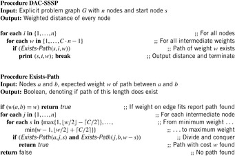
If there is a path with total weight w then it can be decomposed into one of these partitions, assuming that the bounds are contained in the interval  . The worst-case reduction on weights is
  .
.
Therefore, the recursion depth is bounded by  , which results in a space requirement of
  integers. As in the BFS case the running time is exponential (scale-up factor C for partitioning the weights).
5.2. Exploring the Search Tree
Search algorithms that do not eliminate duplicates necessarily view the set of search tree nodes as individual elements in search space. Probably the best way to explain how they work is to express the algorithms as a search in a space of paths. Search trees are easier to analyze than problem graphs because for each node there is a unique path to it.
In other words, we investigate a state space in the form of a search tree (formally a tree expansion of the graph rooted at the start node s), so that elements in the search space are paths. We mimic the tree searching algorithms and internalize their view.
Recall that to certify optimality of the A* search algorithm, we have imposed the admissibility condition on the weight function that for all
  . In the context of search trees, this assumption translates as follows. The search tree problem space is characterized by a set of states S, where each state is a path starting at s. The subset of paths that end with a goal node is denoted by
  . For the extended weight function
  , admissibility implies that
 for all paths
  .
.
Definition 5.1
(Ordered Search Tree Algorithm) Let  be the maximum weight of any prefix of a given path
  ; that is,
 An ordered search tree algorithm expands paths with regard to increasing values of
  .
.
Lemma 5.1
If w is admissible, then for all solution paths  , we have
  .
.
Proof
If  for all
  in S, then for all
  with
with  in S we have
  , especially for path
  with
with  . This implies
  . On the other side,
  and, therefore,
  .
.
The following theorem states conditions on the optimality of any algorithm that operates on the search tree.
Theorem 5.1
(Optimality of Search Tree Algorithms) Let G be a problem graph with admissible weight function w. For all ordered search tree algorithms operating on G it holds that when selecting  we have
  .
.
Proof
Assume  ; that is, there is a solution path
  with
with  that is not already selected. When terminating this implies that there is an encountered unexpanded path
  with
with  . By Lemma 5.1 we have
  in contradiction to the ordering of the search tree algorithm and the choice of pt.
5.3. Branch-and-Bound
Branch-and-bound (BnB) is a general programming paradigm used, for example, in operations research to solve hard combinatorial optimization problems. Branching is the process of spawning subproblems, and bounding refers to ignoring partial solutions that cannot be better than the current best solution. To this end, lower and upper bounds L and U are maintained. Since global control values on the solution quality improve over time, branch-and-bound is effective in solving optimization problems, in which a cost-optimal assignment to the problem variables has to be found.
For applying branch-and-bound search to general state space problems, we concentrate on DFS extended with upper and lower bounds. In this context, branching corresponds to the generation of successors, so that DFS can be casted as generating a branch-and-bound search tree. We have already seen that one way of obtaining a lower bound L for the problem state u is to apply an admissible heuristic h, or  for short. An initial upper bound can be obtained by constructing any solution, such as one established by a greedy approach.
As with standard DFS, the first solution obtained might not be optimal. With DFBnB, however, the solution quality improves over time together with the global value U until eventually the lower bound  at some node u is equal to U. In this case an optimal solution has been found, and the search terminates.
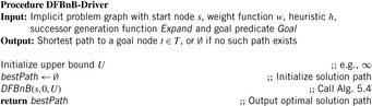
The implementation of DFBnB is shown in Algorithm 5.3. At the beginning of the search, the procedure is invoked with the start node and with the upper bound U set to some reasonable estimate (it could have been obtained using some heuristics; the lower it is, the more can be pruned from the search tree, but in case no upper bound is known, it is safe to set it to  ). A global variable bestPath keeps track of the actual solution path.
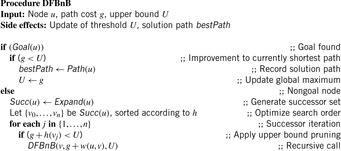
The recursive search routine is depicted in Algorithm 5.4. Sorting the set of successors according to increasing L-values is an optional refinement to the algorithm that often aids in accelerating the search for finding an early solution.
Theorem 5.2
(Optimality Depth-First Branch-and-Bound) Algorithm depth-first branch-and-bound is optimal for admissible weight functions.
Proof
If no pruning was taking place, every possible solution would be generated so that the optimal solution would eventually be found. Sorting of children according to the L-values has no influence on the algorithm's completeness. Condition  confirms that the node's lower bound is smaller than the global upper bound. Otherwise, the search tree is pruned, since admissible weight functions exploring the subtree cannot lead to better solutions than the one stored with U.
An important advantage of branch-and-bound algorithms is that we can control the quality of the solution to be expected, even if it is not yet found. The cost of an optimal solution is only up to  smaller than the cost of the best computed one.
A prototypical example for DFBnB search is the TSP, as introduced in Chapter 1. As one choice for branching, the search tree may be generated by assigning edges to a partial tour. A suboptimal solution might be found quickly.
Consider the TSP of Figure 5.1 together with the Minimum Spanning Tree heuristic. The corresponding branch-and-bound search tree is shown in Figure 5.2. We have chosen an asymmetric interpretation and a branching rule that extends a partial tour by an edge if possible. If in case of a tie the left child is preferred, we see that the optimal solution was not found on the first trial, so the first value for U is 15. After a while the optimal tour of cost 14 is found. The example is too small for the lower bound to prune the search tree based on condition  .
.

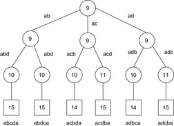 |
| Figure 5.2 Branch-and-bound-tree for TSP of Figure 5.1. |
5.4. Iterative-Deepening Search
We have seen that the first solution found by DFBnB doesn't have to be optimal. Moreover, if the heuristic bounds are weak, the search can turn into exhaustive enumeration. Depth-first iterative-deepening (DFID) tries to control these aspects. The search mimics a breadth-first search with a series of depth-first searches that operate with a successively increasing search horizon. It combines optimality of BFS with the low space complexity of DFS. A successively increasing global threshold U for the solution cost is maintained, up to which a recursive DFS algorithm has to expand nodes.
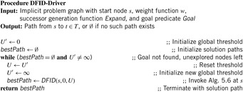
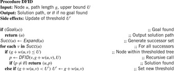
The main driver loop (see Alg. 5.5) maintains U and  , the bound for the next iteration. It repeatedly calls the DFID subroutine of Algorithm 5.6, which searches for an optimal goal path
  in the thresholded search tree. It updates the global variable
  to the minimal weight of all generated, except unexpanded nodes in the current iteration, and yields the new threshold U for the next iteration. Note that if the graph contains no goal and is infinite, then the algorithm will run forever; however, if it is finite, then the f-values also are bounded, and so when U reaches this value,
  will not be updated, it will be
  after the last search iteration. In contrast to A*, DFID can track the solution path on the stack, which allows predecessor links to be omitted (see Ch. 2).
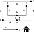
Consider the example of Figure 5.3, a weighted version of a sample graph introduced in Chapter 1. Table 5.1 traces the execution of DFID on this graph. The contents of the search frontier in the form of pending calls to the subroutine are provided. For the sake of conciseness, we assume that the predecessor of a node u is not generated again (as a successor of u) and that the update of value  takes part before the recursive call.
| Step | Iteration | Selection | Pending Calls | U | U′ | Remarks |
|---|---|---|---|---|---|---|
| 1 | 1 | {} | {(a, 0)} | 0 | ∞ | |
| 2 | 1 | a | {} | 0 | 2 | g(b), g(c), and g(d) > U |
| 3 | 2 | {} | {(a, 0)} | 2 | ∞ | New iteration starts |
| 4 | 2 | a | {(b, 2)} | 2 | 6 | g(c) and g(d) > U |
| 5 | 2 | b | {} | 2 | 6 | g(e) and g(f) > U |
| 6 | 3 | {} | {(a,0)} | 6 | ∞ | New iteration starts |
| 7 | 3 | a | {(b, 2), (c, 6)} | 6 | 10 | g(d) > U |
| 8 | 3 | b | {(e, 6), (f, 6), (c, 6)} | 6 | 10 | |
| 9 | 3 | e | {(f, 6), (c, 6)} | 6 | 10 | g(f) > U |
| 10 | 3 | f | {(c, 6)} | 6 | 10 | g(e) > U |
| 11 | 3 | c | {} | 6 | 9 | g(d) |
| 12 | 4 | {} | {(a, 0)} | 9 | ∞ | New iteration starts |
| 13 | 4 | a | {(b, 2), (c, 6)} | 9 | 10 | g(d) > U |
| 14 | 4 | b | {(c, 6), (e, 6), (f, 6)} | 9 | 10 | |
| 15 | 4 | c | {(e, 6), (f, 6), (d, 9)} | 9 | 10 | |
| 16 | 4 | e | {(f, 6), (d, 9), (f, 9)} | 9 | 10 | |
| 17 | 4 | f | {(d, 9), (f, 9), (e, 9)} | 9 | 10 | |
| 18 | 4 | d | {(f, 9), (e, 9)} | 9 | 10 | g(g) and g(c) > U |
| 19 | 4 | f | {(e, 9)} | 9 | 10 | g(b) > U |
| 20 | 4 | e | {(d, 9)} | 9 | 10 | g(b) > U |
| ⋮ | ⋮ | ⋮ | ⋮ | ⋮ | ⋮ | ⋮ |
| 44 | 7 | {} | {(a, 0)} | 14 | ∞ | New iteration starts |
| 45 | 7 | a | {(b, 2), (c, 6), d(10)} | 14 | ∞ | |
| 46 | 7 | b | {(c, 6), (d, 10), (e, 6), (f, 6)} | 14 | ∞ | |
| 47 | 7 | c | {(d, 10), (e, 6), (f, 6))} | 14 | ∞ | |
| 48 | 7 | d | {(e, 6), (f, 6), (e, 9), (c, 13)} | 14 | 15 | g(g) > U |
| 49 | 7 | e | {(f, 6), (d, 9), (c, 13), (f, 9)} | 14 | 15 | |
| 50 | 7 | f | {(d, 9), (c, 13), (f, 9), (e, 9)} | 14 | 15 | |
| 51 | 7 | d | {(c, 13), (f, 9), (e, 9), (g, 14)} | 14 | 15 | |
| 52 | 7 | c | {(f, 9), (e, 9), (g, 14)} | 14 | 15 | g(a) > U |
| 53 | 7 | f | {(e, 9), (g, 14), (b, 13)} | 14 | 15 | |
| 54 | 7 | e | {(g, 14), (b, 13), (b, 13)} | 14 | 15 | |
| 55 | 7 | g | {(b, 13), b(13)} | 14 | 15 | Goal reached |
Theorem 5.3
(Optimality Depth-First Iterative Deepening) Algorithm DFID for unit cost graphs with admissible weight function is optimal.
Proof
We have to show that by assuming uniform weights for the edges DFID is ordered. We use induction over the number of while iterations k. Let  be the set of newly encountered paths in iteration k and
  be the set of all generated but not expanded paths. Furthermore, let
  be the threshold of iteration k. After the first iteration, for all
  we have
  . Furthermore, for all
  we have
  . Let
. Let  for all
  . This implies
  for all q in
  . Hence,
  . For all
  we have
  . Therefore, for all
  the condition
  is satisfied. Hence, DFID is ordered.
5.5. Iterative-Deepening A*
Iterative deepening A* (IDA*) extends the idea of DFID to heuristic search by including the estimate h. IDA* is the most often used alternative in cases when memory requirements are not allowed to run A* directly. As with DFID, the algorithm is most efficient if the implicit problem graph is a tree. In this case, no duplicate detection is required and the algorithm consumes space linear in the solution length.
Algorithm 5.7 and Algorithm 5.8 provide a recursive implementation of IDA* in pseudo code: The value  is the weight of the edge
  , and
, and  and
and  are the heuristic estimate and combined cost for node u, respectively. During one depth-first search stage, only nodes that have an f-value no larger than U(the current threshold) are expanded. At the same time, the algorithm maintains an upper bound
  on the threshold for the next iteration. This threshold is determined as the smallest f-value of a generated node that is larger than the current threshold, U. This minimum increase in the bound ensures that at least one new node is explored in the next iteration. Moreover, it guarantees that we can stop at the first solution encountered. This solution must indeed be optimal due, since no solution was found in the last iteration with an f-value smaller than or equal to U, and
  is the minimum cost of any path not explored before.
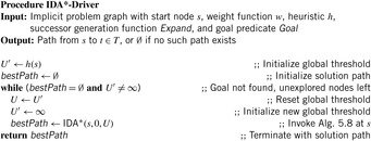

Table 5.2 traces the execution of DFID on our example graph. Note that the heuristic drastically reduces the search effort from 55 steps in DFID to only 7 in IDA*.
| Step | Iteration | Selection | Pending Calls | U | U′ | Remarks |
|---|---|---|---|---|---|---|
| 1 | 1 | {} | {(a, 11)} | 11 | ∞ | h(a) |
| 2 | 1 | a | {} | 11 | 14 | f(b), f(d), and f(c) larger than U |
| 3 | 2 | {} | {(a, 11)} | 14 | ∞ | New iteration starts |
| 4 | 2 | a | {(c, 14)} | 14 | 15 | f(b), f(d) > U |
| 5 | 2 | c | {(d, 14)} | 14 | 15 | |
| 6 | 2 | d | {(g, 14)} | 14 | 15 | f(a) > U |
| 7 | 2 | g | {} | 14 | 15 | Goal found |
The more diverse the f-values are, the larger the overhead induced through repeated evaluations. Therefore, in practice, iterative deepening is limited to graphs with a small number of distinct integral weights. Still, it performs well in a number of applications. An implementation of it using the Manhattan distance heuristic solved random instances of the Fifteen-Puzzle for the first time. Successor nodes that equal a node's predecessor are not regenerated. This reduces the length of the shortest cycle in the resulting problem graph to 12, such that at least for shallow searches the space is “almost” a tree.
Theorem 5.4
(Optimality Iterative-Deepening A*) Algorithm IDA* for graphs with admissible weight function is optimal.
Proof
We show that IDA* is ordered. We use induction over the number of while iterations k. Let  be the set of newly encountered paths in iteration k and
  be the set of all generated but not expanded paths. Furthermore, let
  be the threshold of iteration k.
After the first iteration, for all  we have
  . Moreover, for all
  we have
  . Let
. Let  for all
  . This implies
  for all q in
  . Hence,
  . For all
  we have
  , since assuming the contrary contradicts the monotonicity of
  , since only paths p with
  are newly expanded. Therefore, for all
  the condition
  is satisfied. Hence, IDA* is ordered.
Unfortunately, if the search space is a graph, then the number of paths can be exponentially larger than the number of nodes; a node can be expanded multiple times, from different parents. Therefore, duplicate elimination is essential. Moreover, in the worst case, IDA* expands only one new node in each iteration. Consider a linear-space search represented by the path  . If
. If  denotes the number of expanded nodes in A*, IDA* will expand
  many nodes. Such worst cases are not restricted to lists. If all nodes in a search tree have different priorities (which is common if the weight function is rational) IDA* also degrades to
  many node expansions.
5.6. Prediction of IDA* Search
In the following we will focus on tree-shaped problem spaces. The reason is that while many search spaces are in fact graphs, IDA* potentially explores every path to a given node, and searches the search tree as explained in Section 5.5; complete duplicate detection cannot be guaranteed due to the size of the search space.
The size of a brute-force search tree can be characterized by the solution depth d, and by its branching factor b. Recall that the branching factor of a node is the number of children it has. In most trees, however, different nodes have different numbers of children. In that case, we define the asymptotic branching factor as the number of nodes at a given depth, divided by the number of nodes at the next shallower depth, in the limit as the depth goes to infinity.
5.6.1. Asymptotic Branching Factors
Consider Rubik's Cube with the two pruning rules described in Section 1.7.2. Recall that we divided the faces of the cube into two classes; a twist of a first face can be followed by a twist of any second face, but a twist of a second face cannot be followed immediately by a twist of the opposite first face. We call nodes where the last move was a twist of a first face type-1 nodes, and those where it was a twist of a second face type-2 nodes. The branching factors of these two types are 12 and 15, respectively, which also gives us bounds on the asymptotic branching factor.
To determine the asymptotic branching factor exactly, we need the proportion of type-1 and type-2 nodes. Define the equilibrium fraction of type-1 nodes as the number of type-1 nodes at a given depth, divided by the total number of nodes at that depth, in the limit of large depth. The fraction of type-2 nodes is one minus the fraction of type-1 nodes. The equilibrium fraction is not  : Each type-1 node generates
  type-1 nodes and
  type-2 nodes as children, the difference being that you can't twist the same first face again. Each type-2 node generates
  type-1 nodes and
  type-2 nodes, since you can't twist the opposite first face next, or the same second face again. Thus, the number of type-1 nodes at a given depth is six times the number of type-1 nodes at the previous depth, plus six times the number of type-2 nodes at the previous depth. The number of type-2 nodes at a given depth is nine times the number of type-1 nodes at the previous depth, plus six times the number of type-2 nodes at the previous depth.
Let  be the fraction of type-1 nodes, and
  the fraction of type-2 nodes at a given depth. If n is the total number of nodes at that depth, then there will be
  type-1 nodes and
  type-2 nodes at that depth. In the limit of large depth, the fraction of type-1 nodes will converge to the equilibrium fraction, and remain constant. Thus, at large depth,
Cross multiplying gives us the quadratic equation  , which has a positive root at
  . This gives us an asymptotic branching factor of
  .
.
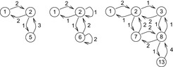
In general, this analysis produces a system of simultaneous equations. For another example, consider the Five-Puzzle, the 2 × 3 version of the well-known sliding-tile puzzles shown in Figure 5.4 (left). In this problem, the branching factor of a node depends on the blank position. The position types are labeled s and c, representing side and corner positions, respectively (see Fig. 5.4, middle). We don't generate the parent of a node as one of its children, to avoid duplicate nodes representing the same state. This requires keeping track of both the current and previous blank positions. Let cs denote a node where the blank is currently in a side position, and the last blank position was a corner position. Define ss, sc, and cc nodes analogously. Since cs and ss nodes have two children each, and sc and cc nodes have only one child each, we have to know the equilibrium fractions of these different types of nodes to determine the asymptotic branching factor. Figure 5.4 (right) shows the different types of states, with arrows indicating the type of children they generate. For example, the double arrow from ss to sc indicates that each ss node generates two sc nodes at the next level.
| Figure 5.4 |
Let  be the number of nodes of type t at depth d in the search tree. Then we can write the following recurrence relations directly from the graph in Figure 5.4. For example, the last equation comes from the fact that there are two arrows from ss to sc, and one arrow from cs to sc.
  The initial conditions are that the first move either generates an ss node and two sc nodes, or a cs node and a cc node, depending on whether the blank starts in a side or corner position, respectively.
A simple way to compute the branching factor is to numerically compute the values of successive terms of these recurrences, until the relative frequencies of different state types converge. Let  ,
,  ,
,  , and
, and  be the number of nodes of each type at a given depth, divided by the total number of nodes at that depth. After a hundred iterations, we get the equilibrium fractions
  ,
,  ,
,  , and
, and  . Since cs and ss states generate two children each, and the others generate one child each, the asymptotic branching factor is
  . Alternatively, we can simply compute the ratio between the total nodes at two successive depths to get the branching factor. The running time of this algorithm is the product of the number of different types of states (e.g., four in this case) and the search depth. In contrast, searching the actual tree to depth 100 would generate over 1013 states.
To compute the exact branching factor, we assume that the fractions eventually converge to constant values. This generates a set of equations, one from each recurrence. Let b represent the asymptotic branching factor. This allows us to rewrite the recurrences as the following set of equations. The last one constrains the fractions to sum to one.

 |
| Figure 5.5 |
For the Twenty-Four-Puzzle, however, the search tree of two side or two middle states may differ. For this case we need six classes with a blank at position 1, 2, 3, 7, 8, and 13 according to the tile labeling in Figure 1.10. In the general case the number of different node branching classes in the (n2 − 1)-Puzzle (without predecessor elimination) is This still compares well to a partition according to the n2 equivalent classes in the first factorization (savings of a factor of about eight) and, of course, to the
  states in the overall search space (exponential savings).
Let F be the vector of node frequencies and P the transposed matrix of the matrix representation of the state-type graph G. Then the underlying mathematical issue turns out to be an eigenvalue problem. Transforming  leads to
  for the identity matrix I. The solutions for b are the roots of the characteristic equation
  where det is the determinant of the matrix. Since
  , the transposition of the equivalence graph matrix preserves the value of b. For the case of the Fifteen-Puzzle with corner, side, and middle nodes, we have
The equation  can be unrolled to
  . We briefly sketch how to compute
  for large values of d. Matrix P is diagonalizable if there exists an inversible matrix C and a diagonal matrix Q with
  . This simplifies the calculation of
  , since we have
  (the remaining terms
  cancel). By the diagonal shape of Q, the value of
  is obtained by simply taking the matrix elements
  to the power of d. These elements are the eigenvalues of P.
For the Fifteen-Puzzle the basis-transformation matrix C and its inverse  are
are and
and The vector of node counts is
 such that the exact total number of nodes in depth d is
 The number of corner nodes (
 ), the number of side nodes (
 ), and the number of middle nodes (
 ) grow as expected. The largest eigenvalue
  dominates the growth of the search tree in the limit for large values of d.
When incorporating pruning to the search, symmetry of the underlying graph structure may be affected. We consider the Eight-Puzzle. The adjacency matrix for predecessor elimination now consists of four classes: cs, sc, mc, and cm, where the class ij indicates that the predecessor of a j-node in the search tree is an i-node, and m stands for the center position.

In the example, the set of (complex) eigenvalues is  ,
,  ,
,  , and
, and  . Therefore, the asymptotic branching factor is
  . The vector
  is equal to
 Finally, the total number of nodes in depth d is
 For small values of d the value
  equals 1, 2, 4, 8, 10, 20, 34, 68, 94, 188, and so on.
Table 5.3 gives the even- and odd-depth branching factors of the (n2 − 1)-Puzzle up to 10 × 10. As n goes to infinity, all the values converge to 3, the branching factor of an infinite sliding-tile puzzle, since most positions have four neighbors, one of which was the previous blank position.
In some problem spaces, every node has the same branching factor. In other spaces, every node may have a different branching factor, requiring exhaustive search to compute the average branching factor. The technique described earlier determines the size of a brute-force search tree in intermediate cases, where there are a small number of different types of states, the generation of which follows a regular pattern.
5.6.2. IDA* Search Tree Prediction
We measure the time complexity of IDA* by the number of node expansions. If a node can be expanded and its children evaluated in constant time, the asymptotic time complexity of IDA* is simply the number of node expansions. Otherwise, it is the product of the number of node expansions and the time to expand a node. Given a consistent heuristic function, both A* and IDA* must expand all nodes of which the total cost,  , is less than c, the cost of an optimal solution. Some nodes with the optimal solution cost may be expanded as well, until a goal node is chosen for expansion, and the algorithms terminate. In other words,
  is a sufficient condition for A* or IDA* to expand node u, and
  is a necessary condition. For a worst-case analysis, we adopt the weaker necessary condition.
An easy way to understand the node expansion condition is that any search algorithm that guarantees optimal solutions must continue to expand every possible solution path, as long as it is smaller than the cost of an optimal solution. On the final iteration of IDA*, the cost threshold will equal c, the cost of an optimal solution. In the worst case, IDA* will expand all nodes u of which the cost  . We will see later that this final iteration determines the overall asymptotic time complexity of IDA*.
We characterize a heuristic function by the distribution of heuristic values over the nodes in the problem space. In other words, we need to know the number of states with heuristic value 0, how many states have heuristic value 1, the number with heuristic value 2, and so forth. Equivalently, we can specify this distribution by a set of parameters D(h), which is the fraction of total states of the problem of which the heuristic value is less than or equal to h. We refer to this set of values as the overall distribution of the heuristic. D(h) can also be defined as the probability that a state chosen randomly and uniformly from all states in the problem space has a heuristic value less than or equal to h. Heuristic h can range from zero to infinity, but for all values of h greater than or equal to the maximum value of the heuristic, D(h) = 1. Table 5.4 shows the overall distribution for the Manhattan distance heuristic on the Five-Puzzle.
The overall distribution is easily obtained for any heuristic. For heuristics implemented in the form of a pattern database, the distribution can be determined exactly by scanning the table. Alternatively, for a heuristic computed by a function, such as Manhattan distance on large sliding-tile puzzles, we can randomly sample the problem space to estimate the overall distribution to any desired degree of accuracy. For heuristics that are the maximum of several different heuristics, we can approximate the distribution of the combined heuristic from the distributions of the individual heuristics by assuming that the individual heuristic values are independent.
The distribution of a heuristic function is not a measure of its accuracy, and says little about the correlation of heuristic values with actual costs. The only connection between the accuracy of a heuristic and its distribution is that given two admissible heuristics, the one with higher values will be more accurate than the one with lower values on average.
Although the overall distribution is the easiest to understand, the complexity of IDA* depends on a potentially different distribution. The equilibrium distribution P(h) is defined as the probability that a node chosen randomly and uniformly among all nodes at a given depth of the brute-force search tree has a heuristic value less than or equal to h, in the limit of large depth.
If all states of the problem occur with equal frequency at large depths in the search tree, then the equilibrium distribution is the same as the overall distribution. For example, this is the case with the Rubik's Cube search tree. In general, however, the equilibrium distribution may not equal the overall distribution. In the Five-Puzzle, for example, the overall distribution assumes that all states, and, hence, all blank positions, are equally likely. At deep levels in the tree, the blank is in a side position in more than one-third of the nodes, and in a corner position in less than two-thirds of the nodes. In the limit of large depth, the equilibrium frequency of side positions is  . Similarly, the frequency of corner positions is
  . Thus, to compute the equilibrium distribution, we have to take these equilibrium fractions into account. The fifth and sixth columns of Table 5.4, labeled corner and side, give the number of states with the blank in a corner or side position, respectively, for each heuristic value. The seventh and eighth columns give the cumulative numbers of corner and side states with heuristic values less than or equal to each particular heuristic value. The last column gives the equilibrium distribution P(h). The probability P(h) that the heuristic value of a node is less than or equal to h is the probability that it is a corner node, 0.64679, times the probability that its heuristic value is less than or equal to h, given that it is a corner node, plus the probability that it is a side node, 0.35321, times the probability that its heuristic value is less than or equal to h, given that it is a side node. For example,
  . This differs from the overall distribution
  .
.
The equilibrium heuristic distribution is not a property of a problem, but of a problem space. For example, including the parent of a node as one of its children can affect the equilibrium distribution by changing the equilibrium fractions of different types of states. When the equilibrium distribution differs from the overall distribution, it can still be estimated from a pattern database, or by random sampling of the problem space, combined with the equilibrium fractions of different types of states, as illustrated earlier.
To provide some intuition behind our main result, Figure 5.6 shows a schematic representation of a search tree generated by an iteration of IDA* on an abstract problem instance, where all edges have unit cost. The numbers were generated by assuming that each node generates one child each with a heuristic value one less, equal to, and one greater than the heuristic value of the parent. For example, there are six nodes at depth 3 with heuristic value 2, one with a parent that has a heuristic value 1, two with parents that have a heuristic value 2, and three with parents that have a heuristic value 3. In this example, the maximum value of the heuristic is 4, and the heuristic value of the initial state is 3.

One assumption of our analysis is that the heuristic is consistent. Because of this, and since all edges have unit cost ( for all u,v) in this example, the heuristic value of a child must be at least the heuristic value of its parent, minus one. We assume a cutoff threshold of eight moves for this iteration of IDA*. Solid arrows represent sets of fertile nodes that will be expanded, and dotted arrows represent sets of sterile nodes that will not be expanded because their total cost,
  , exceeds the cutoff threshold.
The values at the far right of Figure 5.6 show the number of nodes expanded at each depth, which is the number of fertile nodes at that depth.  is the number of nodes in the brute-force search tree at depth i, and P(h) is the equilibrium heuristic distribution. The number of nodes generated is the branching factor times the number expanded.
Consider the graph from top to bottom. There is a root node at depth 0, which generates N1 children. These nodes collectively generate N2 child nodes at depth 2. Since the cutoff threshold is eight moves, in the worst case, all nodes n of which the total cost  will be expanded. Since 4 is the maximum heuristic value, all nodes down to depth
  will be expanded. Thus, for
  , the number of nodes expanded at depth d will be Nd, the same as in a brute-force search. Since 4 is the maximum heuristic value,
  , and, hence,
  .
.
The nodes expanded at depth 5 are the fertile nodes, or those for which  , or
, or  . At sufficiently large depths, the distribution of heuristic values converges to the equilibrium distribution. Assuming that the heuristic distribution at depth 5 approximates the equilibrium distribution, the fraction of nodes at depth 5 with
  is approximately
  . Since all nodes at depth 4 are expanded, the total number of nodes at depth 5 is N5, and the number of fertile nodes is
  .
.
There exist nodes at depth 6 with heuristic values from 0 to 4, but their distribution differs from the equilibrium distribution. In particular, nodes with heuristic values 3 and 4 are underrepresented relative to the equilibrium distribution, because these nodes are generated by parents with heuristic values from 2 to 4. At depth 5, however, the nodes with heuristic value 4 are sterile, producing no offspring at depth 6, hence reducing the number of nodes at depth 6 with heuristic values 3 and 4. The number of nodes at depth 6 with  is completely unaffected by any pruning however, since their parents are nodes at depth 5 with
  , all of which are fertile. In other words, the number of nodes at depth 6 with
  , which are the fertile nodes, is exactly the same as in the brute-force search tree, or
  .
.
Due to consistency of the heuristic function, all possible parents of fertile nodes are themselves fertile. Thus, the number of nodes to the left of the diagonal line in Figure 5.6 is exactly the same as in the brute-force search tree. In other words, heuristic pruning of the tree has no effect on the number of fertile nodes, although it does effect the sterile nodes. If the heuristic was inconsistent, then the distribution of fertile nodes would change at every level where pruning occurred, making the analysis far more complex.
When all edges have unit cost, the number of fertile nodes at depth i is  , where Ni is the number of nodes in the brute-force search tree at depth i, d is the cutoff depth, and P is the equilibrium heuristic distribution. The total number of nodes expanded by an iteration of IDA* to depth d is
 Let us now generalize this result to nonunit edge costs. First, we assume that there is a minimum edge cost; we can, without loss of generality, express all costs as multiples of this minimum cost, thereby normalizing it to one. Moreover, for ease of exposition these transformed actions and heuristics are assumed to be integers; this restriction can easily be lifted.
We replace the depth of a node by  , the sum of the edge costs from the root to the node. Let Ni be the number of nodes u in the brute-force search tree with
  . We assume that the heuristic is consistent, meaning that for any two nodes u and v,
  , where
  is the cost of an optimal path from u to v.
Theorem 5.5
(Node Prediction Formula) For larger values of c the expected number  of nodes expanded by IDA* up to cost c, given a problem-space tree with Ni nodes of cost i, with a heuristic characterized by the equilibrium distribution P, is
Proof
Consider the nodes u for which  , which is the set of nodes of cost i in the brute-force search tree. There are Ni such nodes. The nodes of cost i that will be expanded by IDA* in an iteration with cost threshold c are those for which
  , or
, or  . By definition of P, in the limit of large i, the number of such nodes in the brute-force search tree is
  . It remains to show that all these nodes in the brute-force search tree are also in the tree generated by IDA*.
Consider an ancestor node v of such a node u. Then there is only one path between them in the tree, and  , where
  is the cost of the path from node v to node u. Since
  , and
, and  ,
,  . Since the heuristic is consistent,
  , where
  is the cost of an optimal path from v to u in the problem graph, and hence,
  . Thus,
  , or
, or  . Since
  ,
,  , or
, or  . This implies that node m is fertile and will be expanded during the search. Therefore, since all ancestors of node u are fertile and will be expanded, node u must eventually be generated itself. In other words, all nodes u in the brute-force search tree for which
  are also in the tree generated by IDA*. Since there can't be any nodes in the IDA* tree that are not in the brute-force search tree, the number of such nodes at level i in the IDA* tree is
  , which implies the claim.
The effect of earlier iterations (small values of c) on the time complexity of IDA* depends on the rate of growth of node expansions in successive iterations. The heuristic branching factor is the ratio of the number of nodes expanded in a search-to-cost threshold c, divided by the nodes expanded in a search-to-cost c − 1, or  , where the normalized minimum edge cost is 1. Assume that the size of the brute-force search tree grows exponentially as
  , where b is the brute-force branching factor. In that case, the heuristic branching factor
  is
is The first term of the numerator,
  , is less than or equal to one, and can be dropped without significantly affecting the ratio. Factoring b out of the remaining numerator gives
 Thus, if the brute-force tree grows exponentially with branching factor b, then the running time of successive iterations of IDA* also grows by a factor of b. In other words, the heuristic branching factor is the same as the brute-force branching factor. In that case, it is easy to show that the overall time complexity of IDA* is
  times the complexity of the last iteration (see Exercises).
Our analysis shows that on an exponential tree, the effect of a heuristic is to reduce search complexity from  to
to  , for some constant k, which depends only on the heuristic function; contrary to previous analyses, however, the branching factor remains basically the same.
5.6.3. *Convergence Criteria
We have not yet looked closely at the convergence conditions of the process for computing the asymptotic branching factor.
The matrix for calculating the population of nodes implies  , with
  being the vector of node sizes of different types. The asymptotic branching factor b is the limit of
  , where
  . We observe that in most cases
  for every
  , where k is the number of state types. Evaluating
  for increasing depth d is exactly what is considered in the algorithm of van Mises for approximating the largest eigenvalue (in absolute terms) of P. The algorithm is also referred to as the power iteration method.
As a precondition, the algorithm requires that P be diagonalizable. This implies that we have n different eigenvalues  and each eigenvalue
  with multiplicity of
  has
has  linear-independent eigenvectors. Without loss of generality, we assume that the eigenvalues are given in decreasing order
  . The algorithm further requires that the start vector
  has a representation in the basis of eigenvectors in which no coefficient according to
  is trivial.
We distinguish the following two cases:  and
and  . In the first case we obtain that (independent of the choice of
  ) the value of
  equals
  . Similarly, in the second case,
  is in fact
  . The cases
  for
for  are dealt with analogously. The outcome of the algorithm and therefore the limit in the number of nodes in layers with difference l is
  , so that once more the geometric mean turns out to be
  .
.
We indicate the proof of the first case only. Diagonalizability implies a basis of eigenvectors  . Due to
  the quotient of
  converges to zero for large values of d. If the initial vector
  with respect to the eigenbasis is given as
  , applying
  yields
  by linearity of P, which further reduces to
  by the definition of eigenvalues and eigenvectors. The term
  will dominate the sum for increasing values of d. Factorizing
  in the numerator and
  in the denominator of the quotient of
  results in an equation of the form
  , where
  is bounded by a constant, since except for the leading term
  , both the numerator and the denominator in R only involve expressions of the form
  . Therefore, to find the asymptotic branching factor analytically, it suffices to determine the set of eigenvalues of P and take the largest one. This corresponds to the results of the asymptotic branching factors in the (n2 − 1)-Puzzle.
5.7. *Refined Threshold Determination
A drawback of IDA* is its overhead in computation time introduced by the repeated node evaluations in different iterations. If the search space is a uniformly weighted tree, this is not a concern: Each iteration explores b times more nodes than the last one, where b is the effective branching factor. If the solution is located at level k, then it holds for the number  of expansion in A* that
 depending on the random location of the solution in the last layer.
On the other hand, IDA* performs between  and
and  expansions in the last iteration like A*, and additional
 expansions in all previous iterations. Thus, ignoring lower-order terms the overhead for
  in the range number of iterations is
 In other words, since the number of leaves in a tree is about
  times larger than the number of interior nodes, the overhead of bounded searches to nonleaf levels is acceptable. However, the performance of IDA* can be much worse for general search spaces. In the worst case, if all merits are distinct, in each iteration only one new node is explored, such that it expands
  nodes. Similar degradation occurs, for example, if the graph is a chain. To speed up IDA* for general graphs, it has been proposed to not always use the smallest possible threshold increase for the next iteration, but to augment it by larger amounts. One thing we have to keep in mind in this case is that we cannot terminate the search at the first encountered solution, since there might still be cheaper solutions in the yet unexplored part of the search iteration. This necessarily introduces overshooting behavior; that is, the expansion of nodes with merit larger than the optimal solution.
The idea is to dynamically adjust the increment such that the overhead can be bounded similarly to the case of the uniform tree. One way to do so is to choose a threshold sequence  such that the number of expansions ni in stage i satisfies
 for some fixed ratio r. If we choose r too small, the number of reexpansions and hence the computation time will grow rapidly; if we choose it too big, then the threshold of the last iteration can exceed the optimal solution cost significantly, and we will explore many irrelevant edges. Suppose that
  for some value p. Then IDA* will perform
  iterations. In the worst case, the overshoot will be maximal if A* finds the optimal solution just above the previous threshold,
  . The total number of expansions is
  , and the ratio ν becomes approximately
  . By setting the derivative of this expression to zero, we find that the optimal value for r is 2; that is, the number of expansions should double from one search stage to the next. If we achieve doubling, we will expand at most four times as many nodes as A*.
The cumulative distribution of expansions is problem dependent; however, the function type is often specific to the class of problems to be solved, whereas its parameters depend on the individual problem instance. We record the runtime information of the sequence of expansion numbers and thresholds from the previous search stages, and then use curve fitting for estimating the number of expansions at higher thresholds. For example, if the distribution of nodes with f-value smaller or equal to threshold c can be adequately modeled according to an exponential formula (for adequately chosen parameters A and B) then to attempt to double the number of expansions we choose the next threshold according to
 This way of dynamically adjusting the threshold such that the estimated number of nodes expanded in the next stage grows by a constant ratio is called RIDA*, for runtime regression IDA*.
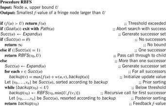
5.8. *Recursive Best-First Search
Algorithms RBFS (recursive best-first search ) and IE (iterative expansion ) were developed independently, but are very similar. Therefore, we will only describe RBFS.
RBFS improves on IDA* by expanding nodes in best-first order, and backing up heuristic values to make the node selection more informed. RBFS expands nodes in best-first order even when the cost function is nonmonotone. Whereas iterative deepening uses a global cost threshold, RBFS uses a local cost threshold for each recursive call. RBFS stores the nodes on the current search path and all their siblings; the set of these nodes is called the search skeleton. Thus, RBFS uses slightly more memory than IDA*, namely  instead of
  , where b is the branching factor of the search tree. The basic observation is that with an admissible heuristic, the backed-up heuristics can only increase. Therefore, when exploring the children of a node, the descendants of the child with lowest f-value should be explored first, until the merits of all nodes in the search frontier exceed the f-value of the second best child. To this end, each node remembers its backup merit, initially set to its f-value. The algorithm is most easily described as a recursive procedure, which takes a node and a bound as arguments (see Alg. 5.9). At the root, it is called with the start node and
  .
.
It has been proposed to augment RBFS such that it can exploit additionally available memory to reduce the number of expansions. The resulting algorithm is called memory-aware recursive best-first search (MRBFS). Whereas the basic RBFS algorithm stores the search skeleton on the stack, in MRBFS the generated nodes have to be allocated permanently; they are not automatically dropped with the end of a recursive procedure call. Only when the overall main memory limit is reached, previously generated nodes other than those on the skeleton are dropped. Three pruning strategies were suggested: pruning all nodes except the skeleton, pruning the worst subtree rooted from the skeleton, or pruning individual nodes with the highest backup value. In experiments, the last strategy was proven to be the most efficient. It is implemented using a separate priority queue for deletions. When entering a recursive call, the node is removed from the queue since it is part of the skeleton and cannot be deleted; conversely, it is inserted upon termination.
5.9. Summary
We showed that divide-and-conquer methods can find optimal solutions with a memory consumption that is only logarithmic in the number of states, which is so small that they cannot even store the shortest path in memory. However, these search methods are impractical due to their large runtime. Depth-first search has a memory consumption that is linear in its depth cutoff since it stores only the path from the root node of the search tree to the state that it currently expands. This allows depth-first search to search large state spaces with a reasonable runtime. We discussed depth-first branch-and-bound, a version of depth-first search that reduces the runtime of depth-first search by maintaining an upper bound on the cost of a solution (usually the cost of the best solution found so far), which allows it to prune any branch of the search tree of which the admissible cost estimate is larger than the current upper bound. Unfortunately, depth-first search needs to search up to the depth cutoff, which can waste computational resources if the depth cutoff is too large, and cannot stop once it finds a path from the start state to any goal state (since the path might not be optimal). Breadth-first search and A* do not have these problems but fill up the available memory on the order of minutes and are thus not able to solve large search problems.
Researchers have addressed this issue by trading off their memory consumption and runtime, which increases their runtime substantially. They have developed a version of breadth-first search, called depth-first iterative-deepening (DFID), and A*, called iterative-deepening A* (IDA*), of which the memory consumption is linear in the length of a shortest path from the start state to any goal state. The idea behind these search methods is to use a series of depth-first searches with increasing depth cutoffs to implement breadth-first search and A*, in the sense that they expand states for the first time in the same order as breadth-first search and A* and thus inherit their optimality and completeness properties. The depth cutoff is set to the smallest depth or f-value of all generated but not expanded states during the preceding depth-first search. Thus, every depth-first search expands at least one state for the first time.
We also discussed a version of IDA* that increases the depth cutoff more aggressively, in an attempt to double the number of states expanded for the first time from one depth-first search to the next one. Of course, DFID and IDA* expand some states repeatedly, both from one depth-first search to the next one and within the same depth-first search. The first disadvantage implies that the runtime of the search methods is small only if every depth-first search expands many states (rather than only one) for the first time. The second disadvantage implies that these search methods work best if the state space is a tree but, in case the state space is not a tree, can be mitigated by not generating those children of a state s in the search tree that are already on the path from the root of the search tree to state s(a pruning method discussed earlier in the context of depth-first search). Note, however, that the information available for pruning is limited since the memory limitation prohibits, for example, to store a closed list.
We predicted the runtime of IDA* in case the state space is a tree. We showed how to compute the number of nodes at a given depth and its asymptotic branching factor, both analytically and numerically, and used this result to predict the number of nodes expanded by IDA* with consistent heuristics. IDA* basically stores only the path from the root node of the search tree to the state that it currently expands. We also discussed recursive best-first search (RBFS), a more sophisticated version of A* of which the memory consumption is also linear in the length of a shortest path from the start state to any goal state (provided that the branching factor is bounded). RBFS stores the same path as IDA* plus all siblings of states on the path and manipulates their f-values during the search, which no longer consists of a series of depth-first searches but still expands states for the first time in the same order as A*, a property that holds even for inadmissible heuristics.
Table 5.5 gives an overview on the algorithms introduced in this chapter. We refer to the algorithm's pseudo code, the algorithm it simulates, and its space complexity. In case of DFID, IDA*, and DFBnB, the complexity  assumes that at most one successor of a node is stored to perform a backtrack. If all successors were stored, the complexity would rise to
  as with RBFS.
5.10. Exercises
5.1 Apply DAC-BFS to the (3 × 3) Gridworld. The start node is located at the top-left and the goal node is located at the bottom-right corner.
1. Protocol all calls to Exists-Path.
2. Report all output due to print.
5.2 We have seen that DFID simulates BFS, and IDA* simulates A*. Devise an algorithm that simulates Dikstra's algorithm. Which assumptions on the weight function are to be imposed?
5.3 Consider the random TSP with 10 cities in Figure 5.7. Solve the problem with depth-first branch-and-bound using:
1. No lower bound.
2. The cost of the Minimum Spanning Tree as a lower bound.

Denote the value of α each time it improves.
5.4 A Maze is an  -size Gridworld with walls. Generate a random maze for small values of n = 100 and m = 200 and a probability of a wall of 30%. Write a program that finds a path from the start to the goal or reports insolvability using:
1. Breadth-first and depth-first search.
2. Depth-first iterative-deepening search.
3. Iterative-deepening A* search with Manhattan distance heuristic.
Compare the number of expanded and generated nodes.
5.6 To see why the even and odd branching factors in the (n2 − 1)-Puzzle are different, color the positions of a puzzle in a checkerboard pattern. If the sets of different-colored squares are equivalent, as in the Five-Puzzle and Fifteen-Puzzle, there is one branching factor. If the sets of different-colored squares are different, however, as in the Eight-Puzzle, there will be different even and odd branching factors.
1. Check the assertion for the 2 × 7 and 4 × 6 board (with predecessor elimination).
2. Prove the assertion.
5.7 Compute the successor generation matrix P for the Eight-Puzzle, Fifteen-Puzzle, and Twenty-Four-Puzzle without predecessor elimination. Take Figure 5.5 as the state-type transition graph.
5.8 Determine the exact node count vectors  of the brute-force search tree in the Eight-Puzzle and Twenty-Four-Puzzle without predecessor elimination by recursively applying the system of recursive equations, starting with a blank in the (top-left) corner.
5.9 Compute the eigenvalues of  and the exact node count vectors
  in the Eight-Puzzle and Twenty-Four-Puzzle without predecessor elimination. Provide the base-transformation matrices. For the Eight-Puzzle this can be done by hand; for the Twenty-Four-Puzzle symbolic mathematical tools are needed.
5.10 Test the theoretical analysis experimentally by predicting the performance of IDA* on the Fifteen-Puzzle using the Manhattan distance heuristic. Use a random sample of a million solvable instances to approximate the heuristic. For  , use the exact numbers of nodes at depth i that are computed from the recurrence relations. Determine the
1. Average heuristic value and maximum number of moves.
2. Average solution length and the relative error of the prediction.
5.11 Show that if the brute-force tree grows exponentially with branching factor b, the overall time complexity of IDA* is  times the complexity of the last iteration.
5.12 Explain where and why consistency of the heuristic is essential in proving Theorem 5.5. What can happen with the successors with regard to the sample tree analysis if we have
1. An admissible but not a consistent estimate?
2. Not even an admissible estimate?
5.13 Provide an example of a state space graph for which RBFS gives a better search result as IDA*.
5.11. Bibliographic Notes
The principle of minimal-space breadth-first and single-source shortest path search is similar to the simulation of nondeterministic Turing machines as proposed by Savitch (1970). For the same restricted memory setting similar problems of node reachability (i.e., determine whether there is any path between two nodes) and graph connectivity have been efficiently solved using random-walk strategies Feige, 1996 and Feige, 1997. Reingold (2005) has developed a deterministic, log-space algorithm that solves the problem of start-to-goal node connectivity in undirected graphs. The result implies a way to construct in log-space a fixed sequence of directions that guides a deterministic walk through all the vertices of any connected graph.
The origins of iterative-deepening search trace back to the late 1960s, when programmers sought a reliable mechanism to control the time consumption of the newly emerging tournament chess programs, so that the search process can halt with the best available answer at hand. IDA* has been invented by Korf (1985a) in the context of solving the Fifteen-Puzzle. In this work Korf provides a list of 100 random problem instances that have been solved with IDA* search. Algorithms that reduce the number of regenerations by increasing the threshold more liberally include IDA*_CR by Russell (1992), DFS* by Rao, Kumar, and Korf (1991) and MIDA* by Wah (1991). The first solution found by these algorithms is often the best possible. Extensions like branch-and-bound are needed to guarantee optimal solutions. Recent results on the predicting IDA* search have been provided by Breyer and Korf (2008).
The analysis of the average branching factor for regular search spaces has been given by Edelkamp and Korf (1998). Search tree prediction for IDA* search, as presented here, has been studied by Korf and Reid (1998). The two aspects have some overlap; a joint exposition has been given by Korf, Reid, and Edelkamp (2001). Exact node counts and sufficient convergence criteria have been given by Edelkamp (2001b). A more complex prediction formula based on including successor values surface in the form of conditional distributions has been provided by Zahavi, Felner, Burch, and Holte (2008a). It extends the analysis discussed in this chapter of the book to the case of inconsistent heuristics, and shows different ways to create more accurate analysis (by considering dependences of different lengths and even making predictions for particular states). Since inconsistency is common in settings such as automated planning and has been proven to be beneficial in others, some work has been already done in predicting the performance of inconsistent heuristic functions by Zahavi, Felner, Schaeffer, and Sturtevant (2007) and by Zhang, Sturtevant, Holte, Schaeffer, and Felner (2009).
Search tree prediction formulas have been used by Holte and Hernádvölgyi (1999) and by Haslum, Botea, Helmert, Bonet, and Koenig (2007) to select expressive pattern databases for the search. Furcy, Felner, Holte, Meshulam, and Newton (2004) exploit the prediction formula to argue why a larger collection of smaller databases often performs better than a smaller collection of large databases. The average solution length for the Fifteen-Puzzle has been computed by Korf and Felner (2002).
Most previous theoretical analyses of heuristic search focused on A*; for example, see the PhD thesis of Gaschnig (1979a), the book of Pearl (1985) and the work of Pohl (1977b). Based on different assumptions, the authors assumed that the effect of a heuristic function is to reduce search complexity from  to
to  , where
  , reducing the effective branching factor. All used an abstract problem-space tree where every node has b children, every edge has unit cost, and there is a single goal node at depth d. The heuristic is characterized by its error in estimating the actual solution cost. This model predicts that a heuristic with constant absolute error results in linear-time complexity, and constant relative error results in exponential time complexity. There are several limitations of this model. The first is that it assumes only one path from the start to the goal state, whereas most problem spaces contain multiple paths to each state. The second limitation is that to determine the accuracy of the heuristic on even a single state, we have to determine the optimal solution cost from that state, which is expensive to compute. Doing this for a significant number of states is impractical for large problems. Finally, the results are only asymptotic, and don't predict actual numbers of node generations.
An attempt for a probabilistic analysis of the A* algorithm has been given by Huyn, Dechter, and Pearl (1980). However, as in similar analyses (e.g., by Sen and Bagchi 1988 and Davis, 1990), the approach only refers to a tree search with A*. The behavior of A* in acyclic graphs that arise in many search problems have been theoretically analyzed by Zhang, Sen, and Bagchi (1999). The authors consider graph structures that arise, for example, in the exploration of Job Sequencing problems and the TSP. To assign a probability distribution on the heuristic estimates, the average analysis is done with respect to three models: linear, less-than-linear, and logarithmic. For the linear model (and some further assumptions), the expected number of distinct nodes is exponential, and for the logarithmic model (and some further assumptions), the number of distinct nodes remains polynomial. A* search using accurate heuristics has been predicted by Dinh, Russell, and Su (2007).
Branch-and-bound has been formulated first by Land and Doig (1960). A simple implementation has been provided by Dakin (1965). Depth-first branch-and-bound in the form of a linear-space search algorithm has been suggested by Korf (1993).
..................Content has been hidden....................
You can't read the all page of ebook, please click here login for view all page.