
Chapter 19. Robotics
Sven Koenig and Craig Tovey
This chapter gives a general introduction to search problems in robotics, including search problems that arise if a robot has incomplete knowledge of its environment or its location in the environment, as is the case for mapping, localization, and goal-directed navigation in unknown terrain. It also discusses different ways of discretizing continuous state spaces.
Keywords: agent-centered search, AND-OR (minimax) search, assumption-based search, conditional plans, configuration space, discretization, goal-directed navigation in unknown terrain, greedy localization, greedy mapping, greedy online search, incomplete knowledge, incremental heuristic search, motion planning, parti-game algorithm, probabilistic roadmaps, rapidly exploring random trees, robot navigation, search with the freespace assumption, tessellation of the plane, visibility graph, Voronoi graph
A difference between search in robotics and typical search testbeds in artificial intelligence, like the Eight-puzzle or the Rubik's cube, is that state spaces in robotics are continuous and need to be discretized. Another difference is that robots typically have a priori incomplete knowledge of the state spaces. In these cases, they cannot predict with certainty which observations they will make after they have moved nor the feasibility or outcomes of their future moves. Thus, they have to search in nondeterministic state spaces, which can be time consuming due to the large number of resulting contingencies. Complete AND-OR searches (i.e., minimax searches) minimize the worst-case trajectory length but are often intractable since the robots have to find large conditional plans. Yet, search has to be fast for robots to move smoothly. Thus, we need to speed up search by developing robot-navigation methods that sacrifice the minimality of their trajectories.
19.1. Search Spaces
Consider the motion-planning problem of changing an unblocked start configuration of a robot to a goal configuration. This is a search problem in the configuration space, where the configuration of a robot is typically specified as a vector of real numbers. For example, the configuration of a mobile robot that is omnidirectional and not subject to acceleration constraints is given by its coordinates in the workspace. Configurations are either unblocked (i.e., possible or, alternatively, in freespace) or blocked (i.e., impossible or, alternatively, part of obstacles). Configurations are blocked, for example, because the robot would intersect an obstacle in the workspace. The configuration space is formed by all configurations.
An example motion-planning problem in a two-dimensional workspace with a robot arm that has two joints and is bolted to the ground at the first joint is shown in Figure 19.1(a). An obstacle blocks one quadrant of the plane. The robot arm has to move from its start configuration to the goal configuration. There are different choices of defining the configuration space. If we only want to find an unblocked trajectory from the start configuration to the goal configuration then the choice is usually unimportant. However, if the planning objective includes the optimization of some cost, such as minimizing time or energy, then it is preferable to define the configuration space so that this cost is represented as a norm-induced or other natural metric on the configuration space. One configuration space is shown in Figure 19.1(b), where the configurations are given by the two joint angles θ1 and θ2. The region in the figure wraps around because angles are measured modulo 360°, so that the four corners in the figure represent the same configuration. Some configurations are blocked because the robot arm would intersect an obstacle in the workspace (but they could also be blocked because a joint angle is out of range). Horizontal movement in the figure requires the robot arm to actuate both joints. Movement along the diagonal with slope one results if only the first joint actuates. Thus, horizontal movement requires more energy than diagonal movement, contrary to what the figure suggests visually. It may then be preferable to define the vertical axis of the configuration space as θ2 − θ1, as shown in Figure 19.1(c).

Robot moves in the workspace are continuous out of physical necessity. The configuration space is therefore continuous and thus needs to get discretized to allow us to use search methods to find trajectories from the start configuration to the goal configuration. We model the configuration space as a (vertex-blocked) graph  , where
  is the set of (blocked and unblocked) vertices,
  is the set of unblocked vertices, and
  is the set of edges. The configuration of the robot is represented by exactly one unblocked vertex at any instant. We say, for simplicity, that the robot visits that vertex. Edges connect vertices that correspond to configurations that the robot can potentially move between. The vertices are blocked or unblocked depending on whether the corresponding configurations are blocked or unblocked. The robot needs to move on a trajectory in the resulting graph from the vertex that corresponds to the start configuration to the vertex that corresponds to the goal configuration. We assume that paths and trajectories do not contain blocked vertices (unless stated otherwise) and measure their lengths as well as all other distances in number of moves (i.e., edge traversals).
We can obtain the graph in different ways.
• We can obtain the graph by partitioning the configuration space into cells (or some other regular or irregular tessellation of the space), where a cell is considered unblocked if and only if it does not contain obstacles. The vertices are the cells and are unblocked if and only if the corresponding cells are unblocked. Edges connect adjacent cells (i.e., cells that share a border) and are thus (about) equally long.
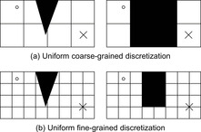
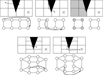
One problem is the granularity of the discretization. If the cells are large, then an existing trajectory might not be found, as shown in Figure 19.2. Blocked configurations are black, and unblocked configurations are white. The circle and cross show the start and goal configuration, respectively. On the other hand, the smaller we make the cells, the more numerous they become, which results in a quadratic explosion. It can therefore make sense to have cells of different sizes: small cells close to obstacles in configuration space to be able to find gaps between them and large cells otherwise. One particular method for obtaining a nonuniform discretization is the parti-game algorithm. It starts with large cells and splits them as needed while trying to move the robot from the start configuration to the cell that contains the goal configuration (goal cell). A simplified version of the parti-game algorithm is illustrated in Figure 19.3. It starts with a uniform coarse-grained discretization of the configuration space. The vertices of the graph represent the cells, and edges connect vertices that correspond to adjacent cells. Thus, it initially ignores obstacles and makes the optimistic assumption that it can move from each cell to any adjacent cell (freespace assumption). It uses the graph to find a shortest path from its current cell to the goal cell. It then follows the path by always moving toward the center of the successor cell of its current cell. If it gets blocked by an obstacle (which can be determined in the workspace and thus without modeling the shape of obstacles in the configuration space), then it is not always able to move from its current cell to the successor cell and therefore removes the corresponding edge from the graph. It then replans and finds another shortest path from its current cell to the goal cell. If it finds such a path, then it repeats the process. If it does not find such a path, then it uses the graph to determine from which cells it can reach the goal cell (solvable cells) and from which cells it cannot reach the goal cell (unsolvable cells, shaded gray in the figure). It then splits all unsolvable cells that border solvable cells (and have not yet reached the resolution limit) along their shorter axes. (It also splits all solvable cells that border unsolvable cells along their shorter axes to prevent adjacent cells from having very different sizes, which is not necessary but makes it efficient to determine the neighbors of a cell with kd-trees.) It deletes the vertices of the split cells from the graph and adds one vertex for each new cell, again assuming that it can move from each new cell to any adjacent cell and vice versa. (It could remember where it got blocked by obstacles to delete some edges from the graph right away but does not. Rather, it deletes the edges automatically when it gets blocked again by the obstacles in the future.) It then replans and finds another shortest path from its current cell to the goal cell and repeats the process until the goal cell is reached or no cell can be split any further because the resolution limit is reached. The final discretization is then used as initial discretization for the next motion-planning problem in the same configuration space.
• We can also obtain the graph by picking a number of unblocked configurations (including the start and goal configurations). The vertices are these configurations and are unblocked. Edges connect vertices of which the connecting straight line (or path of some simple controller) does not pass through obstacles (which can perhaps be determined in the workspace and thus without modeling the shapes of obstacles in the configuration space). We can leave out long edges (e.g., edges longer than a threshold) to keep the graph sparse and the edges about equally long. In case all obstacles are polygons, we can pick the corners of the polygons as configurations (in addition to the start and goal configurations). The resulting graph is called the visibility graph. A shortest trajectory in the visibility graph is also a shortest trajectory in a two-dimensional configuration space (but not necessarily in a three- or higher-dimensional configuration space). However, the obstacles are often not polygons and can only be approximated with complex polygons, resulting in a large number of configurations and thus large search times. Probabilistic roadmaps therefore pick a number of unblocked configurations randomly (in addition to the start and goal configurations). The larger the number of picked configurations, the larger the search time tends to be. On the other hand, the larger the number of picked configurations, the more likely it is that a trajectory is found if one exists and the shorter the trajectory tends to be. So far, we assumed that the configuration space is first discretized and then searched. However, it is often faster to pick random configurations during the search. Rapidly exploring random trees, for example, grow search trees by picking configurations randomly and then try to connect them to the search tree.
There are also other models of the configuration space, for example, Voronoi graphs, which have the advantage that trajectories remain as far away from obstacles as possible and the safety distance to obstacles is thus maximal.
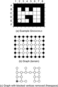
By definition, the robot cannot leave the connected component of unblocked vertices in which it starts. We therefore assume that the graph has only one component of unblocked vertices (i.e., that there is a path between any two unblocked vertices). We draw our examples principally from robot-navigation problems in (two-dimensional four-neighbor) grid graphs, where the configuration space is the workspace itself, and thus use the terms “terrain” and “position” in the following instead of “configuration space” and “configuration.” In general, grid graphs model (two-dimensional four-neighbor) Gridworlds of square cells. Gridworlds (including evidence and occupancy grids) are widely used to model the terrain of mobile robots by partitioning it into square cells, lend themselves readily to illustration, and form challenging testbeds for search under a priori incomplete knowledge.
19.2. Search under Incomplete Knowledge
We assume that the graph is undirected and make the following minimal assumptions about the robot capabilities throughout this chapter, called the base model: The robot is able to move from its current vertex to any desired adjacent unblocked vertex. The robot is capable of error-free moves and observations. For example, it can identify its absolute position with GPS or its relative position with respect to its start position with dead-reckoning (which keeps track of how the robot has moved in the terrain). The robot is able to identify vertices uniquely, which is equivalent to each vertex having a unique identifier that the robot might a priori not know. The robot is able to observe at least the identifier and blockage status of its current vertex and all vertices adjacent to its current vertex. The robot always makes the same observation when it visits the same vertex. The robot is able to remember the sequence of moves that it has executed and the sequence of observations it has made in return.
The base model guarantees that the robot can maintain the subgraph of the graph, including the vertices (with their identifiers and their blockage status) and the edges (i.e., vertex neighborships) that the robot either a priori knew about or has observed already. In a minimal base model, the robot is able to observe exactly the identifier of its current vertex and the identifier and blockage status of all vertices adjacent to its current vertex. We will give an example of a robot that has the capabilities required by the minimal base model shortly in the context of Figure 19.4.
19.3. Fundamental Robot-Navigation Problems
Robots typically have a priori only incomplete knowledge of their terrain or their current position. We therefore study three fundamental robot-navigation problems under a priori incomplete knowledge that underlie many other robot-navigation problems.
Mapping means to obtain knowledge of the terrain, often the blockage status of all positions, called a map. There are two common approaches of handling a priori incomplete knowledge of the terrain. The first approach of handling incomplete knowledge of the terrain is characterized by the robot a priori knowing the topology of the graph. The second approach of handling a priori incomplete knowledge of the terrain is characterized by the robot a priori not knowing anything about the graph, not even its topology.
The objective of the robot is to know everything about the graph that it possibly can, including its topology and the blockage status of every vertex. The robot either a priori knows the topology of the graph and the identifier of each vertex but not which vertices are blocked (Assumption 1) or neither the graph nor the identifier or blockage status of each vertex (Assumption 2). Assumption 1 is a possible assumption for grid graphs, and Assumption 2 is a possible assumption for grid graphs, visibility graphs, probabilistic roadmaps, and Voronoi graphs. The graph can contain blocked and unblocked vertices under Assumption 1 but contains only unblocked vertices under Assumption 2.
An example Gridworld is shown in Figure 19.4(a). Blocked cells (and vertices) are black, and unblocked cells are white. The circle shows the current cell of the robot. We assume that the robot has only the capabilities required by the minimal base model. It always observes the identifier and blockage status of the adjacent cells in the four compass directions and then moves to an unblocked adjacent cell in one of the four compass directions, resulting in a grid graph. This grid graph is shown in Figure 19.4(b) for Assumption 1 and in Figure 19.4(c) for Assumption 2. Initially, the robot knows that it visits cell E2 and observes that cells E1 and F2 are blocked and cells E3 and D2 are unblocked. We denote this observation using a “+” for an unblocked adjacent cell and a “−” for a blocked adjacent cell in the compass directions north, west, south, and east (in this order). Thus, the initial observation of the robot is denoted as “D2 +, E1 −, F2 −, E3 +” or “+ − − +” in short.
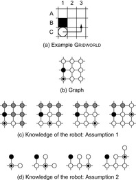
The example in Figure 19.5 shows that it can make a difference whether we make Assumption 1 or 2. The robot moves along the arrow. Figures 19.5(c) and (d) show the knowledge of the robot. Cells (and vertices) that the robot knows to be blocked are black, cells (and vertices) that the robot knows to be unblocked are white, and cells (and vertices) of which the blockage status is unknown to the robot are gray. The circle shows the current cell of the robot. The robot needs to enter the center cell to rule out the possibility that it operates in the graph shown in Figure 19.6 under Assumption 2. On the other hand, it does not need to enter the center cell to know the graph under Assumption 1.
Localization means to identify the current position of a robot, usually a mobile robot rather than a robot arm. We assume that the robot has a map of the terrain available and a priori knows its orientation relative to the map (e.g., because it is equipped with a compass) but not its start position. The robot a priori knows the graph, including which vertices are blocked. Its objective is to localize, which means to identify its current vertex or the fact that its current vertex cannot be identified uniquely because the a priori known map has at least two isomorphic connected components of unblocked vertices and it is located in one of them. The robot a priori does not know the identifier of each vertex. Thus, the robot is not trivially localized after it observes the identifier of a vertex. This assumption is, for example, realistic if the robot uses dead-reckoning to identify the vertices.
Goal-directed navigation in a priori unknown terrain means to move a robot to a goal position in a priori unknown terrain. The robot a priori knows the topology of the graph and the identifier of each vertex but not which vertices are blocked. It knows the goal vertex but may not know the geometric embedding of the graph. Its objective is to move to the goal vertex.
19.4. Search Objective
We perform a worst-casefigtwentytwo analysis of the trajectory length because robot-navigation methods with small worst-case trajectory lengths always perform well, which matches the concerns of empirical robotics researchers for guaranteed performance. We describe upper and lower bounds on the worst-case trajectory length in graphs with the same number of unblocked vertices. The lower bounds are usually proved by example and thus need to be derived scenario by scenario since the trajectories depend on both the graph and the knowledge of the graph. The upper bounds, however, hold for all scenarios of topologies of graphs and observation capabilities of the robot that are consistent with the base model.
Researchers sometimes use online rather than worst-case criteria to analyze robot-navigation methods. For example, they are interested in robot-navigation methods with a small competitive ratio. The competitive ratio compares the trajectory length of a robot to the trajectory length needed by an omniscient robot with complete a priori knowledge to verify that knowledge. For localization, for example, the robot a priori knows its current vertex and only needs to verify it. Minimizing the ratio of these quantities minimizes regret in the sense that it minimizes the value of k such that the robot could have localized k times faster if it had a priori known its current vertex. The competitive ratio has little relation to the worst-case trajectory length if robots do not have complete a priori knowledge. Furthermore, the difference in trajectory length between robot-navigation methods that do and do not have a priori complete knowledge is often large. For goal-directed navigation, for example, the robot can follow a shortest path from the start vertex to the goal vertex if it a priori knows the graph, but usually has to try out many promising paths on average to get from the start vertex to the goal vertex if it a priori does not know the graph. This trajectory length can increase with the number of unblocked vertices while the shortest path can remain of constant length, making the competitive ratio arbitrarily large.
19.5. Search Approaches
A robot is typically able to observe the identifier and blockage status of only those vertices that are close to its current vertex. The robot thus has to move in the graph to observe the identifier and blockage status of new vertices, either to discover more about the graph or its current vertex. Therefore, it has to find a reconnaissance plan that determines how it should move to make new observations, which is called sensor-based search. The reconnaissance plan is a conditional plan that can take into account the a priori knowledge of the robot and the entire knowledge that it has already gathered (namely, the sequence of moves that it has executed and the sequence of observations it has made in return) when determining the next move of the robot. A deterministic plan specifies the move directly while a randomized plan specifies a probability distribution over the moves. No randomized plan that solves one of the robot-navigation problems has a smaller average worst-case trajectory length (where the average is taken with respect to the randomized choice of moves by the randomized plan) than a deterministic plan with minimal worst-case trajectory length. We therefore consider only deterministic plans.
The robot can either first determine and then execute a complete conditional plan (offline search) or interleave partial searches and moves (online search). We now discuss these two options in greater detail, using localization as an example. Localization consists of two phases, namely hypothesis generation and hypothesis elimination. Hypothesis generation determines all vertices that could be the current vertex of the robot since they are consistent with the current observation made by it. This phase simply involves going through all unblocked vertices and eliminating those that are inconsistent with the observation. If the set contains more than one vertex, hypothesis elimination then tries to determine which vertex in this set is the current vertex by moving the robot in the graph. We discuss in the following how hypothesis elimination can use search to determine how to move the robot.
19.5.1. Optimal Offline Search
Offline search finds a complete and thus potentially large conditional plan before the robot starts to move. A valid localization plan eventually correctly identifies either the current vertex of the robot or the fact that the current vertex cannot be identified uniquely, no matter which unblocked vertex the robot starts in.
Consider, for example, the localization problem from Figure 19.7. Figure 19.8 shows part of the state space that the robot can move to from the start state. The states are sets of cells, namely the cells that the robot could be in. Initially, the robot observes “+ − − −”. The question marks indicate the cells that are consistent with this observation, namely cells E2, E4, and E6. The start state thus contains these three cells. (The robot can rule out cell B7 since it knows its orientation relative to the map.) Every state that contains only one cell is a goal state. In every nongoal state, the robot can choose a move (OR nodes of the state space), described as a compass direction. It then makes a new observation (AND nodes of the state space). The state space is nondeterministic since the robot cannot always predict the observation and thus the successor state resulting from a move.

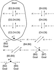
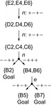
Deterministic localization plans assign a move to each OR node in the state space. Valid deterministic localization plans with minimal worst-case trajectory length can be found with a complete AND-OR search (i.e., minimax search), resulting in decision trees (i.e., trees where the root is the start state, all leaf nodes are goal states, every AND node has all of its successor nodes included, and every OR node has at most one of its successor nodes included) since states cannot repeat in valid localization plans with minimal worst-case trajectory length. Such a decision tree is shown in Figure 19.9. However, it is intractable to perform a complete AND-OR search. This is not surprising since the states are sets of unblocked vertices and their number is thus large (although not all sets of unblocked vertices can appear in practice). In fact, it is NP-hard to localize with minimal worst-case trajectory length and thus very likely needs exponential search time, which is consistent with results that show the complexity of offline search under a priori incomplete knowledge to be high in general.
19.5.2. Greedy Online Search
To search fast, we need to speed up search by developing robot-navigation methods that sacrifice the minimality of their trajectories. If done correctly, the suboptimality of the trajectory and thus the increase in the execution time are outweighed by the decrease of the search time so that the sum of search and execution times (i.e., the problem-completion time) decreases substantially, which is the idea behind limited rationality. For robot-navigation problems under a priori incomplete knowledge, this can be done by interleaving searches and moves to obtain knowledge about the graph or the current vertex in the graph early and then using this knowledge for the new searches right away. This knowledge makes subsequent searches faster since it reduces the uncertainty of the robot about the graph or its current vertex, which reduces the size of the state space that the robot can move to from its current state and thus also the amount of search performed for unencountered situations.
Search in deterministic state spaces is fast. Greedy online search makes use of this property to solve search problems in nondeterministic state spaces by interleaving myopic searches in deterministic state spaces and moves. The result is a trade-off between search and execution time. We now introduce two greedy online search approaches, namely agent-centered search and assumption-based search. They differ in how they make search deterministic.
Agent-centered search methods (in nondeterministic state spaces) search with limited lookahead by performing partial AND-OR searches, forward from the current state, instead of a complete one. They restrict the search to the part of the state space around the current state (resulting in local search), which is the part of the state space that is immediately relevant for the robot in its current situation because it contains the states that the robot will soon be in. Thus, agent-centered search methods decide on the part of the state space to search and then how to move within it. Then, they execute these moves (or only the first move) and repeat the overall process from the resulting state. Consequently, agent-centered search methods avoid a combinatorial explosion by finding only prefixes of complete plans.
Since agent-centered search methods do not search all the way from the current state of the robot to a goal state, they need to avoid moving in a way that cycles forever. The agent-centered search methods that we describe in this chapter do this by making the lookahead large enough so that the subsequent execution obtains new knowledge, although real-time heuristic search methods can be used to get away with smaller lookaheads. Furthermore, the agent-centered search methods that we describe in this chapter use a simple approach to make search fast, namely by searching exactly in all of the deterministic part of the non-deterministic state space around the current state, with the objective to execute a move with more than one possible successor state and thus obtain new knowledge quickly. This is the part of the state space in Figure 19.8 that has a border around it. The robot then traverses the path, the last move of which has more than one possible successor state. It then observes the resulting state and repeats the process from the state that actually resulted from the move instead of all states that could have resulted from it.
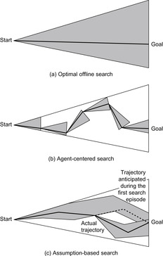
Figure 19.10(b) illustrates agent-centered search. The shaded areas represent the search spaces of agent-centered search, one for each search episode between consecutive moves. The shaded areas together are much smaller than the shaded area of the large triangle in Figure 19.10(a) that represents the search space of an optimal offline search method but the resulting trajectory is not shortest.
Assumption-based search methods, on the other hand, search all the way from the current state to a goal state but make assumptions about the successor states of moves by ignoring some of them. Therefore, assumption-based search methods find a complete plan (under the assumptions made) from the current state to the goal state and execute the plan. If a move results in a successor state that was ignored during the search, then they repeat the overall process from the state that resulted from the move. Consequently, assumption-based search methods avoid a combinatorial explosion because they ignore some successor states of moves and thus do not consider all contingencies. The agent-centered search methods that we describe in this chapter use a simple approach to make search fast, namely by ignoring all successor states of each move but one, which makes the state space effectively deterministic.
Figure 19.10(c) illustrates assumption-based search. The shaded areas represent the search spaces of assumption-based search, one for each search episode. The shaded areas together are much smaller than the shaded area of the large triangle in Figure 19.10(a) that represents the search space of an optimal offline search method but the resulting trajectory is not shortest.
Greedy online robot-navigation methods are commonsense robot-navigation methods that have often been discovered and implemented by empirical robotics researchers. We study greedy localization, greedy mapping, and search with the freespace assumption. They are related and can be analyzed in a common framework.
19.6. Greedy Localization
Greedy localization uses agent-centered search to localize a robot. Greedy localization maintains a set of hypotheses, namely the unblocked vertices that the robot could be in because they are consistent with all previous observations. It always reduces the size of this set with as few moves as possible, until this is no longer possible. This corresponds to moving on a shortest path from its current vertex to a closest informative vertex until it can no longer move to an informative vertex. We define an informative vertex to be an unblocked vertex with the property that the robot can obtain knowledge about its current vertex that allows it to reduce the size of its set of hypotheses. Note that a vertex becomes and remains uninformative once the robot has visited it.
Figure 19.7 illustrates the trajectory of greedy localization. Initially, it can be in cells E2, E4, and E6. The fastest way to reduce the size of the set of hypotheses in this situation is to move north twice. It could then observe “− − + +”, in which case it must be in cell B2. It could also observe “− + + +”, in which case it can be in cells B4 and B6. Either way, it has reduced the size of its set of hypotheses. After the robot executes the moves, it observes “− + + +” and thus can be in cells B4 and B6. The fastest way to reduce the size of its set of hypotheses in this situation is to move east. It could then observe “− + − +”, in which case it must be in cell B5. It could also observe “− + − −”, in which case it must be in cell B7. Either way, it has reduced the size of its set of hypotheses. After the robot executes the move, it observes “− + − +” and thus knows that it is cell B5 and has localized, in this particular case with minimal worst-case trajectory length.
Greedy localization can use deterministic search methods and has low-order polynomial search times in the number of unblocked vertices because it performs an agent-centered search in exactly all of the deterministic part of the nondeterministic state space around the current state, namely exactly up to the instant when it executes a move that has more than one possible successor state and then reduces the size of its set of hypotheses, as shown with a border in Figure 19.8.
It is NP-hard to localize better than logarithmically close to minimal worst-case trajectory length, including in grid graphs. Moreover, robots are unlikely to be able to localize in polynomial time with a trajectory length that is within a factor  of minimal. We analyze the worst-case trajectory length of greedy localization as a function of the number of unblocked vertices, where the worst case is taken over all graphs of the same number of unblocked vertices (perhaps with the restriction that localization is possible), and all start vertices of the robot and all tie-breaking strategies are used to decide which one of several equally close informative vertices to visit next. The worst-case trajectory length of greedy localization is
  moves in graphs
  under the minimal base model and thus is not minimal. This statement continues to hold in grid graphs where localization is possible. It is
  moves in graphs
  and thus is rather small. These results assume that the graph has only one connected component of unblocked vertices but that the a priori known map of the graph can be larger than the graph and contain more than one connected component of unblocked vertices.
moves in graphs 19.7. Greedy Mapping
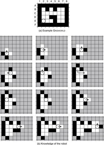
Greedy mapping uses agent-centered search to learn a graph. The robot a priori knows either the topology of the graph and the identifier of each vertex but not which vertices are blocked or neither the graph nor the identifier or blockage status of each vertex. The robot maintains the currently known subgraph of the graph, regardless of what other knowledge it obtains. It always moves on a shortest path from its current vertex to a closest informative vertex in the currently known subgraph until it cannot move to an informative vertex any longer. We define an informative vertex to be an unblocked vertex with the property that the robot can obtain new knowledge for its map in it. Note that a vertex becomes and remains uninformative once the robot has visited it. (An alternative version of greedy mapping always moves to a closest unvisited vertex.)
Figure 19.11 illustrates the trajectory of greedy mapping if the robot a priori knows the topology of the graph and the identifier of each vertex but not which vertices are blocked. Arrows show the paths determined by greedy mapping whenever greedy mapping determines them. The robot then traverses these paths without search, and an arrow is thus only shown for the first move on each path. Greedy mapping can use deterministic search methods and has a low-order polynomial search time in the number of unblocked vertices because it performs an agent-centered search in exactly all of the deterministic parts of the nondeterministic state space around the current state, namely exactly up to the instant when it executes a move that has more than one possible successor state and thus obtains new knowledge for its map. Greedy mapping has to search frequently. It can calculate the shortest paths from the current vertex to a closest informative vertex efficiently with incremental heuristic search methods, which combine two principles for searching efficiently, namely heuristic search (i.e., using estimates of the goal distances to focus the search) and incremental search (i.e., reusing knowledge obtained during previous search episodes to speed up the current one).
We analyze the worst-case trajectory length of greedy mapping as a function of the number of unblocked vertices, where the worst case is taken over all graphs of the same number of unblocked vertices, and all possible start vertices of the robot and all possible tie-breaking strategies are used to decide which one of several equally close informative vertices to visit next. The worst-case trajectory length of greedy mapping is  moves in graphs
  under the minimal base model in case the robot a priori knows neither the graph nor the identifier or blockage status of each vertex. This statement continues to hold in grid graphs in case the robot a priori knows the topology of the graph and the identifier of each vertex but not which vertices are blocked. This lower bound shows that the worst-case trajectory length of greedy mapping is slightly superlinear in the number of unblocked vertices and thus not minimal (since the worst-case trajectory length of depth-first search is linear in the number of unblocked vertices). The worst-case trajectory length of greedy mapping is also
  moves in graphs
  , whether the robot a priori knows the topology of the graph or not. The small upper bound is close to the lower bound and shows that there is only a small penalty to pay for the following qualitative advantages of greedy mapping over depth-first search. First, greedy mapping is reactive to changes of the current vertex of the robot, which makes it easy to integrate greedy mapping into complete robot architectures because it does not need to have control of the robot at all times. Second, it is also reactive to changes in the knowledge that the robot has of the graph since each search makes use of all of the knowledge that the robot has of the graph. It takes new knowledge into account immediately when it becomes available and changes the moves of the robot right away to reflect its new knowledge.
moves in graphs Uninformed real-time heuristic search methods can also be used for mapping graphs but their worst-case trajectory lengths are typically  moves or worse in graphs
  , whether the robot a priori knows the topology of the graph or not, and thus is larger than the ones of greedy mapping.
19.8. Search with the Freespace Assumption
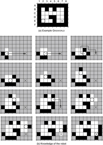
Search with the freespace assumption uses assumption-based search for goal-directed navigation in a priori unknown terrain. Search with the freespace assumption maintains the blockage status of the vertices that the robot knows so far. It always moves on a shortest presumed unblocked path from its current vertex to the goal vertex until it visits the goal vertex or can no longer find a presumed unblocked path from its current vertex to the goal vertex. A presumed unblocked path is a sequence of adjacent vertices that does not contain vertices that the robot knows to be blocked. The robot moves on the presumed unblocked path toward the goal vertex but immediately repeats the process if it observes a blocked vertex on the planned path. Thus, it repeatedly makes the first move on a shortest presumed unblocked path from the current vertex to the goal vertex. This allows it to either follow the path successfully or obtain knowledge about the graph. If the robot visits the goal vertex, it stops and reports success. If it fails to find a presumed unblocked path from its current vertex to the goal vertex, it stops and reports that it cannot move to the goal vertex from its current vertex and, since the graph is undirected, neither from its start vertex.
Figure 19.12 illustrates the trajectory of search with the freespace assumption. The cross shows the goal cell. Search with the freespace assumption can use deterministic search methods and has a low-order polynomial search time in the number of vertices (but not necessarily unblocked vertices). It can calculate the shortest presumed unblocked paths efficiently with incremental heuristic search methods. The computational advantage of incremental heuristic search methods, such as D* (Lite), over search from scratch is much larger for search with the freespace assumption than for greedy mapping.
We analyze the worst-case trajectory length of search with the freespace assumption as a function of the number of unblocked vertices, where the worst case is taken over all graphs of the same number of unblocked vertices, and all start and goal vertices of the robot and all tie-breaking strategies are used to decide which one of several equally short presumed unblocked paths to move along. The worst-case trajectory length of search with the freespace assumption is  moves in graphs
  under the minimal base model and thus is not minimal since the worst-case trajectory length of depth-first search is linear in the number of unblocked vertices. This statement continues to hold in grid graphs. It is
  moves in graphs
  and
and  moves in planar graphs
  , including grid graphs. The small upper bound is close to the lower bound and shows that there is only a small penalty to pay for the following qualitative advantages of search with the freespace assumption over depth-first search. First, search with the freespace assumptions attempts to move in the direction of the goal vertex. Second, it reduces its trajectory length over time (although not necessarily monotonically) when it solves several goal-directed navigation problems in the same terrain and remembers the blockage status of the vertices that the robot knows so far from one goal-directed navigation problem to the next one. Eventually, it moves along a shortest trajectory to the goal vertex because the freespace assumption makes it explore vertices with unknown blockage status and thus might result in the discovery of shortcuts.
moves in graphs 19.9. Bibliographic Notes
Overviews on motion planning and search in robotics have been given by Choset et al. (2005), LaValle (2006), and, for robot navigation in unknown terrain, Rao, Hareti, Shi, and Iyengar (1993). The parti-game algorithm has been described by Moore and Atkeson (1995). Greedy online search is related to sensor-based search, which has been described by Choset and Burdick (1994). It can be implemented efficiently with incremental heuristic search methods, including D* by Stentz (1995a) and Stentz (1995b) and D* Lite by Koenig and Likhachev (2005); see also the overview by Koenig, Likhachev, Liu, and Furcy (2004).
Greedy localization has been described and analyzed by Mudgal, Tovey, and Koenig (2004); Tovey and Koenig (2000); and Tovey and Koenig (2010). It is implemented by the Delayed Planning Architecture (with the viable plan heuristic) by Genesereth and Nourbakhsh (1993) and Nourbakhsh (1997). Variants of greedy localization have been used by Fox, Burgard, and Thrun (1998) and Nourbakhsh (1996). Minimax LRTA* by Koenig (2001a) is a real-time heuristic search method that generalizes the Delayed Planning Architecture to perform agent-centered searches in only a part of the deterministic part of the nondeterministic state space. It deals with the problem that it might then not be able to reduce the size of its set of hypotheses and thus needs to avoid infinite cycles with a different method, namely real-time heuristic search. The NP-hardness of localization has been analyzed by Dudek, Romanik, and Whitesides (1998) and Koenig, Mitchell, Mudgal, and Tovey (2009). Guibas, Motwani, and Raghavan (1992) gave a geometric polynomial time method for robots with long-distance sensors in continuous polygonal terrain to determine the set of possible positions that are consistent with their initial observation. Localization has been studied principally with respect to the competitive ratio criterion of Sleator and Tarjan (1985), starting with Papadimitriou and Yannakakis (1991). Examples include Baeza-Yates, Culberson, and Rawlins (1993); Dudek, Romanik, and Whitesides (1998); Fleischer, Romanik, Schuierer, and Trippen (2001); and Kleinberg (1994).
Greedy mapping has been described and analyzed by Koenig, Smirnov, and Tovey (2003) and Tovey and Koenig (2003). Variants of greedy mapping have been used by Thrun et al. (1998); Koenig, Tovey, and Halliburton (2001b); and Romero, Morales, and Sucar (2001). Mapping with depth-first search has been described by Wagner, Lindenbaum, and Bruckstein (1999). Mapping has been studied principally with respect to the competitive ratio criterion. Examples include Deng, Kameda, and Papadimitriou (1998); Hoffman, Icking, Klein, and Kriegel (1997); Albers and Henzinger (2000); and Deng and Papadimitriou (1990).
Search with the freespace assumption has been described by Stentz (1995b) and described and analyzed by Koenig, Smirnov, and Tovey (2003); Mudgal, Tovey, Greenberg, and Koenig (2005); and Mudgal, Tovey, and Koenig (2004). Variants of search with the freespace assumption have been used by Stentz and Hebert (1995) and, due to their work and follow-up efforts, afterwards widely in DARPA's unmanned ground vehicle programs and elsewhere. Goal-directed navigation in a priori unknown terrain has been studied principally with respect to the competitive ratio criterion. Examples include Blum, Raghavan, and Schieber (1997) and Icking, Klein, and Langetepe (1999). The most closely related results to the ones described in this chapter are the bug algorithms by Lumelsky and Stepanov (1987).
..................Content has been hidden....................
You can't read the all page of ebook, please click here login for view all page.