
Integrated Sensor Systems and Data Fusion for Homeland Protection
Alfonso Farina*, Luciana Ortenzi*, Branko Ristic† and Alex Skvortsov†, *SELEX Electronic Systems, Rome, Italy, †DSTO, Melbourne, Vic. 3207, Australia
Abstract
This chapter addresses the application of data and information fusion to the design of integrated systems in the Homeland Protection (HP) domain. HP is a wide and complex domain: systems in this domain are large (in terms of size and scope) integrated (each subsystem cannot be considered as an isolated system) and different in purpose. Such systems require a multidisciplinary approach for their design and analysis and they are necessarily required to provide data and information fusion in the most general sense. The first data fusion algorithms employed in real systems in the radar field go back to the early seventies; now a days new concepts have been developed and spread to be applied to very complex systems with the aim to achieve the highest level of intelligence as possible and hopefully to support decision. Data fusion is aimed to enhance situation awareness and decision making through the combination of information/data obtained by networks of homogeneous and/or heterogeneous sensors. The aim of this chapter is to give an overview of the several approaches that can be followed to design and analyze systems for homeland protection. Different fusion architectures can be drawn on the basis of the employed algorithms: they are analyzed under several aspects in this chapter. Real study cases applied to real world problems of homeland protection are provided in the chapter.
Keywords
Data fusion; Information fusion; Homeland protection; Sensor network; Collaborative signal and information processing; Self-organizing sensor network; Cooperative sensor network; Network centric operations; Sensor deployment; Tracking; Classification; Situation awareness
Acknowledgments
The first two authors wish to warmly thank Prof F. Zirilli (Univ. of Rome) for his contribution to Section 2.22.6.1, Dr. S. Gallone (SELEX Sistemi Integrati) for contributing to Section 2.22.8.2 and Dr. A. Graziano (SELEX Sistemi Integrati) for the continuous and fruitful cooperation on the many topics described in the Chapter for years.
2.22.1 Introduction
As stated by John Naisbitt in his bestseller “Megatrends” [1], published in 1982, about the new trends and directions transforming our lives: “We are drowning in information but starved for knowledge. This level of information is clearly impossible to be handled by present means. Uncontrolled and unorganized information is no longer a resource in an information society, instead it becomes the enemy.” This successful sentence can be taken as a statement of the problem of information fusion: how can knowledge, awareness and decision making capability be achieved starting from the available information?
This chapter is intended as an attempt to technical and mathematical answer to the previous question; in particular it addresses the application of data and information fusion to the design of integrated systems in the Homeland Protection (HP) domain. HP refers to the broad civilian and military effort produced by a Country to protect its territory—including citizens, assets and activities which are vital and fundamental for its growth and prosperity—against internal and external hazards and to reduce its vulnerability to attacks, whatever their origin, as well as natural disasters. HP is therefore a wide and complex domain: systems in this domain are large, to mean that size and scope of such systems are conspicuous and that system boundaries may not be easy to identify; systems are integrated, to mean that it is generally not sufficient to study each subsystem in isolation; systems are different in purpose and require a multidisciplinary approach for their design and analysis.
The design and analysis of such systems devoted to operate in such scenarios are necessarily required to provide data and information fusion in the most general sense. Information fusion is about combining, or fusing, information from different sources to provide knowledge that is not evident from individual sources. Numerous real world problems benefit from the combination of heterogeneous information sources, for instance, as depicted in Figure 22.1, multi-sensor data fusion is naturally performed by animals and humans to access more accurately the surrounding environment and to identify threats or food, thereby improving their chances of survival. The field of information fusion is commonly characterized as multidisciplinary research area and includes and/or overlaps with a number of other areas. The information fusion at sensor level includes signal processing; at data level data processing; at meta-data level it overlaps with knowledge representation and, finally, at the decision level it involves the decision making capability. Data fusion has been defined in [2] as “the process of combining evidence to support intelligence generation.” Mainly the methods employed to achieve this scope can be divided into two general classes: quantitative and qualitative. The former are based on numerical techniques, the latter ones are based on symbolic representation of information.
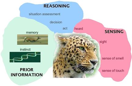
Figure 22.1 Why information fusion. (Kindly provided by Dr. A. Benavoli—IDSIA, Istituto Dalle Molle di Studi sull’Intelligenza Artificiale, Switzerland.)
Examples of quantitative methods can be found in stochastic estimation theory, that aim to estimate the state of a system, using all available information, and to characterize the fusion uncertainty in the framework of probability theory. Most of the algorithms developed for quantitative fusion are based on Bayes filter [3], as Kalman filter [4], information filter [5] and neural networks. The application of these algorithms is employed usually to perform multi-target and multi-sensor tracking. The new generation methods, applying a qualitative approach, are based on a symbolic representation of information. They are, of course, based on mathematical models and their output is numeric, however they can be employed to model qualitative information (e.g., fuzzy). They include expert systems, heuristic, behavioral and structural modeling. Qualitative methods are based on artificial intelligence techniques, such fuzzy logic [6], Dempster-Shafer theory [7,8] Dezert-Smarandache theory [9,10] and rules based-methods.
The first data fusion algorithms employed in real systems in the radar field go back to the early seventies, when they had been developed for multi-radar tracking (MRT) for netted sensors. It was late 1970s, beginning 1980s when these new algorithms and the corresponding means to mitigate unavoidable sources of errors due to practical world (e.g., the time synchronization, the radar alignment to the North, the inaccurate knowledge of coordinates of radar sites) were provided. Probably one of the first MRT system for Air Traffic Control (ATC) ever installed was the system operating in the center and South of Italy [11]. When the competence on tracking was so mature, it was collected in a brand new book on radar data processing [12,13], translated also in Russian and Chinese.
Later in 1990s further advancements were done in the field of multi-sensor fusion for Airborne Early Warning (AEW) systems, setting up an algorithm suite to track targets on the basis of the data provided by surveillance radar, an Identification Friend or Foe (IFF), an Electronic Support Measurement (ESM) and data links. After conceiving also algorithms to track targets on the basis of the angle and identification measurements provided by ESM on a moving platform, data fusion of active and passive tracks was provided [14–17].
Nowadays concepts have been developed and spread to be applied to very complex systems with the aim to achieve the highest level of intelligence as possible and hopefully to support decision. Data fusion is aimed to enhance situation awareness and decision making through the combination of information/data obtained by networks of homogeneous and/or heterogeneous sensors. A sensor network presents advantages over a single sensor under different points of views, as it supplies both redundant and complementary information. Redundant information is exploited to make the system robust to the failure in order that a malfunction of an entity of the system means only a degradation of the performances, rather than the complete failure of the system, since information about the same environment can be obtained from different sources. More robustness can be achieved also with respect to interferences, both intentional and unintentional, due to frequency and spatial diversity of the sensors. Complementary information build up a more complete picture of the observed system; for example sensors are dislocated over large regions providing diverse viewing angles of observed phenomenon and different technologies can be employed in the same application to provide improved system performance.
A large number of different applications, algorithms and architectures have been developed exploiting these advantages. Several examples can be found in robotics, military applications, Homeland Protection and management of large and complex critical infrastructures. Although the specific nature of each problem is different, the final goal, from the point of view of the sensed information, is always the same: using all the available data to better understand the investigated phenomena. The aim of this chapter is to give an overview of the several approaches that can be followed to design and analyze systems for Homeland Protection. Different fusion architectures can be drawn on the basis of the employed algorithms; according to this approach, three general categories can be identified in the literature [18,19]: centralized, hierarchical, and decentralized/netcentric.
The traditional architecture is centralized: in this framework several sensing devices are connected to a central component, the fusion node. For example, in the case of a sensor network employed for the surveillance of an area, usually the information traffic goes from the sensor nodes to a single sink node called information fusion center. According to the information received from the sensors, the fusion center monitors the area where the sensors are deployed and decides the actions to take. Conceptually, the algorithms employed in this case are relatively simple and the resource allocation is straightforward because the central component has an overall view of the whole system. This kind of architecture presents several drawbacks: high computational load, the possibility of catastrophic failure when the fusion node goes down and the lack of flexibility to changes of the system and sensor entities. Therefore this approach is still valid if the number of sensors, whose information is fused, independently of the width of the area to be monitored, is limited and also the relationship and interconnections among sensors are limited too.
In hierarchical architectures, there are several fusion nodes, where intermediate fusion processes are performed, and an ending central fusion node. The principle of a hierarchy is to reduce the communications and computational loads of centralized systems by distributing data fusion tasks among a hierarchy of sensor entities. However in a hierarchy there is still a central component acting as a fusion center. Entities constituting local fusion center, locally process information and send it to the central fusion node. This approach is commonly used in robotics and surveillance applications. Although this architecture reduces the computational and communication loads, there are still some drawbacks connected to the centralized model. In addition to these problems, there are some disadvantages related to the resource allocation balancing and the vulnerability to communication bottlenecks.
In certain cases the traditional data fusion algorithms may still be valid; however, in some cases the great variety of sub-systems and the complexity of interconnections may require new approaches. Most of the drawbacks of centralized and hierarchical architectures can be overcame by decentralized architectures. The trend in surveillance today is towards Network Centric Operation (NCO) [20]. The vision for NCO is to provide seamless access to timely information to all operators (e.g., soldier, officer) and decision-makers at every echelon in the military hierarchy. The goal is to enable all elements, including individual infantry soldiers, ground vehicles, command centers, aircraft and naval vessels, to share the collected information and to combine it into a coherent, accurate picture of the battlefield.
The same approach can be followed in the organization of a sensor network. In recent years the decreasing sensor cost and the development of telecommunication technology have made possible the deployment of networks with a huge number of sensors; in this case the use of information fusion centers is unpractical. Consequently a new class of sensor networks, whose way of functioning is called network centric, has emerged. These networks do not have a fusion center and their functioning is based on the information exchange between near-by sensors. Under this approach the information can be considered as a property of the network rather than of the own sensor. This solution is strongly advocated for its robustness and ease of implementation, but it might suffer when the number of sensors grows very much. It has a broad range of potential applications in the field of Homeland Protection: surveillance of habitat and environmental monitoring, structural monitoring (e.g., bridges), contaminants, smart roads, intruder detection, battlefield. It is complementary to the classical surveillance with few large-costly sensors hierarchically organized.
The network of numerous sensors and communication nodes (for instance: peer to peer networks) may have link topology varying with time due to natural interferences, electromagnetic propagation masked by the terrain surface, meteorological conditions, dust and smoke which might be present in the environment, allowing therefore modularity, robustness and flexibility. These networks should be designed to be resilient to Electronic Counter Measures (ECM), cyber attacks and should be able to manage increasing and highly variable flow of data. The satisfaction of such demanding requirements, maintaining however the limitation of resources such as energy, bandwidth and node complexity, can be achieved borrowing from biological systems several mechanism. For example bio-inspired sensor networks employ decentralized decisions through the self-synchronization mechanism observed in nature that allows forcing every single node of the network to reach the globally optimal decision, without the need of any fusion center. However there are also drawbacks associated to these architectures: in fully decentralized systems, communication issues are more complex and depend on the topology of the network; generally, communication overheads are higher than in centralized systems.
In this chapter these aspects will be investigated in depth for networks respectively of homogeneous and heterogeneous sensors with the description of real study cases applied to real world problems of Homeland Protection. In particular the possibility of netting different sensors operating with different characteristics of domain, coverage, frequency and resolution allows a multi-scale1 approach. This approach is particularly suitable for the surveillance of wide areas such as national borders or critical strategic regions.
The chapter is organized as follows: Section 2.22.2 illustrates the Homeland Protection domain and highlights some of the characteristics of systems in this specific domain; Section 2.22.3 briefly reviews the development of data fusion and gives references to new emerging trends in the domain of high level data fusion. Section 2.22.4 gives a broad and very general description of the basic categories of intelligence that are the source of data and information employed to perform the fusion process. The Sections 2.22.5 and 2.22.6 tackle different aspects related to homogeneous sensor networks. The former proposes several issues from a theoretical point of view, illustrating, next to traditional approaches, the new trends of Collaborative Signal and Information Processing (CSIP), self-organizing and self-synchronizing sensor network; Section 2.22.5 proposes also some remarks about real applications and the need to rethink some mathematical algorithms to overcome the network centric approach. The latter, Section 2.22.6, proposes three real study cases where the novel approaches give significant results. Likewise Section 2.22.7 tackles the aspects related to heterogeneous sensor networks, dealing with the problems of deployment, behavior assignment and coordination of the different sensors. Also in this case a special attention is focused on the mathematical issues related to these new approaches. Real applications of this kind of sensor networks are described in Sections 2.22.8 and 2.22.9, respectively for the border control problem and the forecasting and estimation of an epidemics. Finally Section 2.22.9, with the concluding remarks, follows.
2.22.2 The Problem of homeland protection
The diagram of Figure 22.2 provides a decomposition of the Homeland Protection domain: the two main sub-domains are Homeland Defense (HD) and Homeland Security (HS) [21].
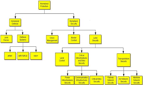
Figure 22.2 Homeland Protection domain. (From [21], reprinted with permission.)
HD includes the typical duties and support systems of military joint forces and single armed forces. Usually HD systems are strictly military, are employed by military personnel only, satisfy specific technical requirements, operational needs and environmental scenarios, and in most cases are designed to face only military threats. The new trend aims to employ military surveillance systems in combined military and civil operations, especially to face terrorism [22]. The military domain has also been swept in recent years by the NCO paradigm; NCO predicates a tighter coupling among forces, especially in the cognitive domain, to achieve synchronization, agility and decision superiority and it is a strong driver in the transformation from a platform-centric force to a network-centric force [20].
HS is a very broad and complex domain that requires coordinated action among national and local governments, private sector and concerned citizens across a country; it covers issues such as crisis management, border control, critical infrastructure protection and transportation security [23,24]. Crisis management is the ability of identifying and assessing a crisis, planning a response, and acting to resolve the crisis situation. Border control aims to build a smart protection belt all around a country to counter terrorism and illegal activities; yet it is not resolutive due to the difficulty of controlling the country boundaries along their full and variegated extension, the non necessarily physical nature of attacks in the current information age, and the threats which often arise internally to the country itself. HS includes also land security that is particularly critical because of its complexity and strategic importance; the security of critical assets, such as electric power plants, communication infrastructures, strategic areas and railway networks, must be ensured continuously in space and time [25–27]. The most recent terrorist attacks have shown the vulnerability of national critical infrastructures [28] and have made the world aware of the possibility of large-scale terrorist offensive actions against civil society: the September 11th, 2001 attack on the World Trade center in New York City is the most dramatic example of this new terrorism. The main emphasis has been put on the terrorist threat, but what emerges is the fragility and vulnerability of modern society to both deliberate threats and natural disasters. Figure 22.3 shows a Synthetic Aperture Radar (SAR) image collected by a satellite of the Italian CosmoSkyMed constellation of the area of the Fukushima nuclear plant hit in 2011 by the tsunami.
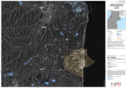
Figure 22.3 A CosmoSkyMed SAR image of Fukushima nuclear plant zone after the tsunami 2011 showing the flooded areas. (Courtesy of E-geos, a Telespazio Company.)
The HP domain includes also the protection from deliberate attacks against the commercial activities of a Country led also out of the national territory, comprehensive also of the territorial waters and Exclusive Economic Zone (EEZ). Seaborne piracy against transport vessels remains a significant issue (with estimated worldwide losses of US$13–16 billion per year), particularly in the waters between the Red Sea and Indian Ocean, off the Somali coast, and also in the Strait of Malacca and Singapore, which are navigated by over 50,000 commercial ships a year [29,30].
The globalization, the pervasiveness of information technologies and the transformation of the industrial sector and civil society have created new vulnerabilities in the system as a whole, but all this has happened without a corresponding effort to increase its robustness and security. As an example, single infrastructure networks have grown over the years independently, creating autonomous “vertical” systems with limited points of contact; around year 2000, as a consequence of the change of trend in the socio-techno scenario, the infrastructures have begun to share services and thus to create interconnected and interdependent systems. Nowadays infrastructures are interconnected and mutually dependent in a complex way: a phenomenon that affects one infrastructure can have a direct or indirect impact on other infrastructures, spreading on a wide geographical area and affecting several sectors of the citizen life. This is schematically represented in Figure 22.4[31,32].
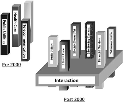
Figure 22.4 Interdependencies between present infrastructures. (From [31], reprinted with permission.)
Beside the physical protection of territory, citizens, critical assets and activities, the security of information and computer systems is one the greatest challenges for a Country. Information and communication technologies have enhanced the efficiency and the comfort of the civil society on one hand, but added complexity and vulnerability on the other hand. The cyber security consists in ensuring the protection of information and property from hackers, corruption, or natural disaster, maintaining however the information and property accessible and productive to its intended users. This problem is pervasive in nearly all the systems supporting a nation: financial, energy, healthcare and transportation. The new trend toward the mobile communications is revealing a new cyber vulnerability, for instance the sheer mass of mobile endpoints gives more protection to hackers leading a cyber attack starting from a mobile. Therefore, the mobile infrastructure is becoming a critical infrastructure as well [33].
Nowadays the challenge is to understand this new scenario and to address the use of new and efficient algorithms for the information fusion in the domain of large integrated systems [34]. To integrate such heterogeneous information the necessity emerges to develop new algorithms of data fusion and information fusion to achieve an operational picture. In such scenario, where the attack can be lead with unconventional manners, information of heterogeneous sources, despite appearing uncorrelated, can be related and hence exploited by its fusion. Therefore particular attention is due to the information sources; Section 2.22.4 is devoted to this aspect of the problem, giving an overview of the sensors and the systems that traditionally provide information.
2.22.3 Definitions and background
Before addressing in more detail the topic of data fusion applied to the domain of Homeland Protection, it is useful to briefly review the evolution of data fusion and, more recently, the definition of the new paradigms and the introduction to high-level data fusion and information fusion.
A definition of data fusion is provided in [35]: “Data fusion is a process that combines data and knowledge from different sources with the aim of maximizing the useful information content, for improved reliability or discriminant capability, while minimizing the quantity of data ultimately retained.” Another definition is provided by the Joint Directors of Laboratories (JDL) Data Fusion Subpanel (DFS) which, in its latest revision of its data fusion model, Steinberg and Bowman [36] settle with the following short definition: “Data fusion is the process of combining data or information to estimate or predict entity states.” Due to its generality, the definition of JDL encompasses the previous one. One aspect of the data fusion process, which is not included in the first definition and is implicit in the second, is process refinement, i.e., the improving of data fusion process and data acquisition. Many authors, recognize process refinement and data fusion to be so closely coupled that process refinement should be considered to be a part of the data fusion process. This is not a new technique in itself, rather a framework for incorporating reasoning and learning with perceived information into systems, utilizing both traditional and new areas of research. These areas include decision theory, management of uncertainty, digital signal processing, and computer science. The data fusion process comprises techniques for data reduction, data association, resource management, and fusion of uncertain, incomplete, and contradictory information.
In 1986, an effort to standardize the terminology related to data fusion began and the JDL data fusion working group was established. The result of that effort was the conception of a process model for data fusion and a data fusion lexicon. The so-called JDL fusion model [37] is a functional model, developed to overcome potential confusion in the community and to improve communications among military researchers and system developers. The model provides a common frame of reference for fusion discussions and to facilitate understanding and recognizing the problems where data fusion is applicable. The first issue of the model, dated 1988, provided four fusion levels:
In 1998 Steinberg et al. [38] revised and expanded the JDL model to broaden the functional model and related taxonomy beyond the original military focus. They introduced a level 0 to the model for estimation and prediction of signal/object observable states on the basis of pixel/signal-level data association and characterization. They also suggested renaming and re-interpretation of level 2 and level 3 to focus on understanding the external world beyond military situation and threat focus. Figure 22.5 reports a block diagram representing this functional model. Although originally developed for military applications, the model is generally applicable. Furthermore, the model does not assume its functions to be automated, they could equally well be maintained by human labor. Hence, the model is both general and flexible. The revised JDL model levels specify logical separations in the data fusion process and divide information into different levels of abstraction depending on the kind of information they produce, where the lower levels yield more specific, and the higher more general, information. The model is divided into the following five levels [18]:
• Level 0—sub-object assessment: the pre-detection activities such as pixel or signal processing, spatial or temporal registration is present. Level 0 deals with the estimation and prediction of signal/object observable states on the basis of pixel/signal level data association and characterization.
• Level 1—object assessment: is concerned with estimation and prediction of target locations, behavior or identity. In this level, which is sometimes referred to as multi-sensor data fusion or multi-sensor integration, data is combined to assign dynamic features (e.g., velocity) as well as static (e.g., identity) to objects, hence adding semantic labels to data. This level includes techniques for data association and management of objects (including creation and deletion of hypothesized objects, and state updates of the same). Level 1 addresses the following functions: data alignment, data/object correlation, object positional/kinematic/attribute estimation, object identity estimation.
• Level 2—situation assessment: investigates the relations among entities such as force structure and communication roles. This level involves aggregation of level 1 entities into high-level, more abstract entities, and relations between entities. An entity in this level might be a pattern of connected objects of level 1 entities. Input data are assessed with respect to the environment, relationship among level 1 entities, and entity patterns in space and time. Level 2 addresses the following functions: object aggregation, contextual interpretation/fusion, event/activity aggregation, multi-perspective assessment.
• Level 3—impact assessment: outlines sets of possible courses of action and the effect on the current situation. The impact assessment, which is sometimes called significance estimation or threat refinement, estimates and predicts the combined effects of system control plans and the entities of level 2 (possibly including estimated or predicted plans of other environment agents) on system objectives. Level 3 addresses the following functions: estimate/aggregate force capabilities, predict enemy intent, identify threat opportunities, estimate implications, multi perspective assessment.
• Level 4—process refinement: is an element of Resource Management used to close the loop by re-tasking resources to support the objectives of the mission. Process refinement evaluates the performance of the data fusion process during its operation and encompasses everything that refines it, e.g., acquisition of more relevant data, selection of more suitable fusion algorithms, optimization of resource usage with respect to, for instance, electrical power consumption. Process refinement is sometimes called process adaption to emphasize that it is dynamic and should be able to evolve with respect both its internal properties and the surrounding environment. The function of this level is in some literature handled by a so called meta-manager or meta-controller. It is also rewarding to compare level 4 fusion to the concept of covert attention in biological vision which involves, e.g., sifting through an abundance of visual information and selecting properties to extract. Level 4 addresses the following functions: evaluation (real-time control/long term improvement), fusion control, source requirements, mission management.
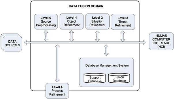
Figure 22.5 JDL model. (From [40], reprinted with permission.)
The 1998 revised JDL fusion model recognized the original Process Refinement level 4 function as a Resource Management function. In 2002, a level 5 was added [39,40], named User Refinement, into the JDL model to support a user’s trust, workload, attention, and situation awareness. Mainly the level 5 was added to distinguish between machine-process refinement and user refinement of either human control action or the user’s cognitive model. In many cases the data fusion process is focused on the machine point of view, however a full advantage can be taken by considering also the human factor, not only as a qualified expert to refine the fusion process, but also as a costumer for whom the fusion system is designed. Figure 22.6, taken from [40], shows the JDL fusion model including also the level 5.
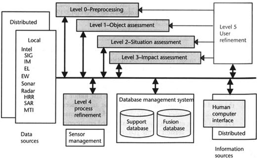
Figure 22.6 JDL model including level 5. (From [40], reprinted with permission.)
Later in [41] also a level 6, Mission Management, was added; this level tackles the adaptive determination of spatial-temporal control of assets (e.g., airspace operations) and route planning and goal determination to support team decision making and actions (e.g., theater operations) over social, economic, and political constraints.
Figure 22.7 shows a multi-sensor data fusion architecture with a representation of the levels involved into each process of data fusion. Level 0 and level 1 concern the combination of data from different sensors, level 2 and level 3 are often referred to as information fusion. Under the proposed partitioning scheme, the same entity can simultaneously be the subject of level 0, 1, 2, and 3 fusion processes. Entity features can be estimated from one or more entity signal observations (e.g., pixel intensities, emitter pulse streams) via a level 0 data preparation/association/estimation process. The identity, location, track and activity state of an entity (whether it be a man, a vehicle, or a military formation) can be estimated on the basis of attributes inferred from one or more observations; i.e., via a level 1 data preparation/association/estimation process. The same entity’s compositional or relational state (e.g., its role within a larger structure and its relations with other elements of that structure) can be inferred via level 2 processes. Thus, a single entity—anything with internal structure, whether man, machine, or mechanized infantry brigade—can be treated either as an individual, subject to level 1 observation and state estimation—or as a “situation,” subject to compositional analysis via level 2 entity/entity association and aggregate state estimation. The impact of a signal, entity, or situation on the user goal or mission can then be predicted based upon an association of these to alternative courses of action for each entity via a level 3 process.
There are also other fusion models developed on the basis of different perspectives, including a purely computational and a human information processing. In the following an overview of different models [42].
The DIKW (Data Information Knowledge and Wisdom) [43] hierarchy organizes data, information, knowledge, and wisdom in layers with an increasing level of abstraction and addition of knowledge, starting from the bottommost data layer. The hierarchy can be considered alike the JDL data fusion model because both start from raw transactional data to yield knowledge at an increasing level of abstraction.
The JDL model and many other computational models do not simulate the complex human cognitive process that leads to “become aware,” because they do not model the fusion process from a human perspective. In 1988, Endsley defined the situation awareness as “the perception of the elements in the environment within a volume of time and space, the comprehension of their meaning, and the projection of their state in the near future” [44]. In [45,46] he identified three levels of situation awareness, namely perception, comprehension, and projection, parallel to the corresponding levels in the JDL model. Therefore the levels in the JDL model can be considered as processes producing results to help a human operator became aware of the situation. In [47] in addition to this three different aspects identified by Endsley, the model included also “intention” (i.e., the understanding of own options and courses of action relative to own goals) and “metacognition” (i.e., accounting for how reliable own situation awareness is likely to be). These levels summarize the fact that situation awareness requires the understanding of information, events, and the impact of own actions on own goals and objectives. This process involves several capabilities as learning, detection of anomalies, prediction of future behaviors, managing uncertainty, and analysis of heterogeneous sources.
The OODA (Observe-Orient-Decide-Act) loop, developed by Boyd in 1987 [48], is one of the first C4I (Command, Control, Communications, Computers, and Intelligence) architectures and it represents the classic decision-support mechanism in military information operations. Because decision-support systems for situational awareness are tightly coupled with fusion systems, the OODA loop has also been used for sensor fusion [49]. Observations in OODA refer to scanning the environment and gathering information from it; orientation is the use of the information to form a mental image of the circumstances; decision is considering options and selecting a subsequent course of action; and action refers to carrying out the conceived decision. Bedworth and O’Brien [50] report a comparison of the OODA loop to the levels of the JDL model.
The human information processing can be modeled by the Rasmussen model [51,52]. It is composed of three layers, namely skill-based, rule-based, and knowledge-based processing. The input of the process is a perception (e.g., the detection of a target by a sensor) and the output is an action. An example of result at the first level may be represented by the automatic identification of a tank by processing of row sensors data; at the next level an enemy unit composition can be indentified on the basis of its number and relative locations. Knowledge-based behavior represents the most complex cognitive processing used to handle novel, complex, situations where no routine or rule is available to manage situations. An example of this type of processing may be the interpretation of unusual behavior, and the consequent generation of a course of actions based on enemy unit size and behavior.
The Generic Error modeling System (GEMS) [53] is an extension of Rasmussen’s approach, which describes the competencies needed by workers to perform their roles in complex systems. GEMS describes three major categories of errors: skill-based slips and lapses, rule-based mistakes, and knowledge-based mistakes.
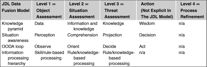
Table 22.1, from [42], shows a correspondence, and not a comparison, among levels and layers of various models presented before. This table is intended as a guide to identify the components of a data fusion architecture, where the separation between the columns is not so sharp. Notice that the JDL model does not explicitly model into a level the action consequent to the threat assessment. The action level, with the sense of a reaction is only in part included in the process refinement level 4, for this reason the column “action” has been inserted in the table, to allow a more clear correspondence with the other models that explicitly account for the reaction. The JDL model is the one that allows the most global view of the data fusion process from an operative perspective: there is not any correspondence of the other models with JDL level 4.
2.22.4 The information sources
This section gives a broad and very general description of the basic categories of intelligence that are the source of data/information employed to perform the fusion process. The USAF (United States Air Force) in 1998 first and the ODNA (Office of Directors of National Intelligence) later in 2008 described in their studies that there are six basic intelligence categories [54,55]:
• Signals Intelligence (SIGINT),
• Imagery Intelligence (IMINT),
• Measurement and Signature Intelligence (MASINT),
• Human Intelligence (HUMINT),
In addition, there is also Scientific and Technical (S&T) Intelligence resulting from the analysis of foreign scientific and technical information. In the following is an overview of the categories.
SIGINT is achieved by the interception/detection of electromagnetic (em) emissions. SIGINT includes Electronic Intelligence (ELINT) and Communications Intelligence (COMINT). The former derives from the processing and analysis of em radiation emitted from emitters, in most of cases radars, not employed for communications, other than nuclear detonations or radioactive sources. An emitter may be related closely to a specific threat. The information that can be achieved by a typical ESM (Electronic Support Measures) device consists of an estimate of the emitter category, location, with a certain accuracy, and various electronic attributes, such as frequency and pulse duration. This information can be employed in a high-level fusion process. COMINT derives from the processing and analysis of intercepted communications from emitters. The communications may be encrypted and they may be of several forms such as voice, e-mail, fax and the like.
IMINT is obtained by sensors working in several bandwidths which are able to produce a view of the scenario or of the specific target: electro/optical sensors, infrared, radar (e.g., Synthetic Aperture Radar (SAR) and Inverse SAR (ISAR), and Moving Target Indicator (MTI)), laser, laser radar (LADAR), and multi-spectral sensors. Each sensor has a unique capability. Some work in all weather conditions, some may work also in night conditions, and some produce high-quality images with detectable signatures.
MASINT is obtained by the collection and the analysis of several and heterogeneous sensors and instruments usually working in different regions or domains of the em spectrum, such as infrared or magnetic fields. MASINT includes Radar Intelligence (RADINT), Nuclear Intelligence (NUCINT), Laser Intelligence (LASINT), and Chemical and Biological Intelligence (CBINT). RADINT, is a specialized form of ELINT, which categorizes and locates as active or passive collection of energy reflected from a target.
HUMINT is the collection of information derived by the human contact. Information of interest might include target name, size, location, time, movement, and intent. HUMINT typically includes structured text (e.g., tables, lists), annotated imagery, and free text (e.g., sentences, paragraphs). HUMINT provides comprehension of adversary actions, capability and capacity, plans and intentions, decisions, research goals and strategies.
OSINT is publicly available information appearing either in print or in electronic form including radio, television, newspapers, journals, the Internet, commercial databases, videos, graphics, and drawings. OSINT can be considered as a complement to the other intelligence categories and can be used to fill gaps and improve accuracy and confidence in classified information. A special mentioning is for the Internet, that, with its blogs, e-mails, videos, messages and mobile systems, favors an ever greater interaction between users. Moreover notice that there is a little overall planning in the development of the World Wide Web, but rather a myriad of initiatives by individuals of small groups. Government have always tried to use telephone tapping, surveillance, files, i.e., intelligence. Now this is possible on a different scale given the technical possibilities offered by satellites, mobile, phones, credit cards management systems, information storage, etc. From the topological point of view, Internet is a scale-free complex network with a power-law of the distribution of the nodes [56]; this technical remark should be considered in the data exploitation analysis.
GEOINT is the analysis and the visual representation of the activities on the earth related to the security achieved by the sensors (radar, optical, IR, multispectral) deployed in the space. The information related to GEOINT is obtained through an integration of imagery, imagery intelligence, and geospatial information.
2.22.5 Homogeneous sensor networks
Stand-alone sensors usually provide a fragmentary view of a complex situation of interest. A significant enhancement of performance can therefore be accomplished by a combination of networked sensors in the close vicinity to the region of interest. Using efficient methods of centralized or decentralized multiple sensor fusion, the quality of the produced situation picture can significantly be improved. In practice, improvements with respect to the following aspects are of interest:
• production of accurate and continuous tracks (e.g., objects, persons, single vehicles, group objects),
• system reaction rates (e.g., track extraction, detection of target maneuvers, track monitoring),
• sustainment of reconnaissance capabilities in case of either system or network failures (e.g., graceful degradation),
• system robustness against jamming and deception,
• compensation of degradation effects (e.g., sensor misalignment, limited sensor resolution),
• robustness against sub-optimal real-time realizations of sensor data fusion algorithms,
• processing of eventually delayed sensor data (e.g., out-of sequence measurements).
In the following, several sections tackle different aspects related to homogeneous sensor networks.
2.22.5.1 Sensor configuration
Sensor fusion networks can be categorized according to the type of sensor configuration. Durrant-Whyte distinguishes three types of sensor configuration as schematized in Figure 22.8 [57,58].
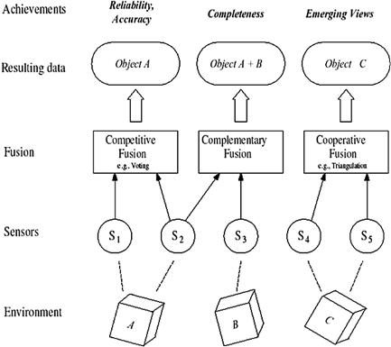
Figure 22.8 Sensors configuration (from [57], reprinted with permission).
Competitive sensor data fusion: Sensors are configured competitive if each sensor delivers independent measurements of the same property. Sensor data represent the same attribute, and the fusion is to reduce uncertainty and resolve conflicts. Competitive sensor configuration is also called a redundant configuration. Sensors S1 and S2 in Figure 22.8 represent a competitive configuration, where both sensors redundantly observe the same property of an object in the environment space.
Complementary sensor data fusion: A sensor configuration is called complementary if the sensors do not directly depend on each other, but can be combined to give a more complete image of the phenomenon under observation. Fusion of the sensor data provides an overall and complete model. Examples for a complementary configuration is the employment of multiple cameras each observing disjoint parts of a room, or using multiple spectrum signatures to identify a land cover type, or using different waveform to identify an aircraft type. Sensor S2 and S3 in Figure 22.8 represent a complementary configuration, since each sensor observes a different part of the environment space.
In both competitive and complementary sensor configurations, there is an improvement of the accuracy of the target characteristics estimation consequent to the data fusion. In their seminal work H. Cramer and C.R. Rao found how to compute the best theoretical accuracy that can be achieved by an estimator. The lower bound of accuracy, i.e., the mean square error of any unbiased estimator, is given by the inverse of the so-called Fisher Information Matrix (FIM). The computation of the CRLB (Cramer-Rao Lower Bound) applies to problems involving the maximum likelihood estimation of unknown constant parameters from noisy measurements [59]. The best achievable improvement of target location and track accuracy can be quantified by the reduction of the CRLB consequent to the track fusion. In [60] this computation is reported in case of fusion of data from two sensors with an ideal unitary detection probability. In [61,62] the same computation has been proposed in case of detection probability less than one and false alarm probability higher than zero.
Cooperative sensor data fusion: A cooperative sensor network uses the information provided by two independent sensors to derive information that would not be available from the single sensors. An example for a cooperative sensor configuration is stereoscopic vision: by combining two-dimensional images from two cameras at slightly different viewpoints a three-dimensional image of the observed scene is derived. Cooperative sensor fusion is the most difficult to design, because the resulting data are sensitive to inaccuracies in all individual participating sensors. Thus, in contrast to competitive fusion, cooperative sensor fusion generally decreases accuracy and reliability. Sensor S4 and S5 in Figure 22.8 represent a cooperative configuration. Both sensors observe the same object, but the measurements are used to form an emerging view on object C that could not have been derived from the measurements of S4 or S5 alone.
These three categories of sensor configuration are not mutually exclusive. Many applications implement aspects of more than one of the three types. An example for such a hybrid architecture is the application of multiple cameras that monitor a given area. In regions covered by two or more cameras the sensor configuration can be competitive or cooperative. For regions observed by only one camera the sensor configuration is complementary.
2.22.5.2 Classical approach to surveillance
Sensor networks have countless applications, for example, we mention the sensor networks used in computer science and telecommunications, in biology, where they can be used to monitor the behavior of animal species such as birds or fishes, and in habitat monitoring, where they can be used to provide real-time rainfall and water level information used to evaluate the possibility of flooding. In the field of Homeland Protection one of the main task to be assigned to a sensor network is the surveillance with its most general significance. Automatic surveillance is a process of monitoring the behavior of selected objects (targets and/or anomalies) inside a specific area by means of sensors. A target generally consists of an object (e.g., a tank close to a land border or a rubber approaching to the coast) whose presence and characteristics can be detected and estimated by the sensor; an anomaly consists in a non usual behavior (e.g., a jeep moving off-road, the increasing of the radioactivity level within an area) that can be revealed by the sensor. Sensors typically provide the following functions:
• detection of a targets or anomalies inside the surveillance area,
• estimation of target position or the anomaly localization and extension,
• monitoring of the target kinematic (tracking) or of the anomaly behaviors,
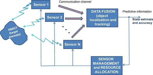
To perform the previous functions, the sensors can be organized on the bases of several approaches. The classical approach to surveillance of wide areas is based on the use of a single or few sensors with long range capabilities. The signal received by the single sensor is processed by means of suitable digital signal processing subsystems. In this case the sensors are costly, with adequate computation and communication capabilities. Sensors are normally located in properly selected sites, to mitigate terrain masking problems; nevertheless, they provide different performance depending on the location of target inside the surveillance area. Typical sensors are radars (ground-based, air-borne, ship-borne or space-based), infrared or TV cameras, seismic, acoustical, radioactive sensors. Usually in this kind of networks, as represented in Figure 22.9, the information traffic goes from the sensor nodes to a single sink node called information fusion center that performs the target localization and tracking. According to the information received from the sensors the fusion center monitors the area where the sensors are deployed and decides, on the basis of the state estimates and their accuracy (e.g., a covariance matrix for a Kalman filter or a particle cloud for a particle filter) the actions to take.
In [63] an example of high-performance radar netted for Homeland Security application with a centralized data fusion process is described. The same classical approach is presented in [64] where this kind of sensor network is employed for natural resource management and bird air strike hazard (BASH) applications.
However if an intruder reaches and neutralizes the fusion center, the communication between the network nodes are interrupted and the whole network is exposed to the risk of becoming useless as a network even if the individual sensors may still be all working.
2.22.5.3 Collaborative signal and information processing (CSIP)
Nowadays, a novel approach to the automatic surveillance has been adopted; it is based on the use of many sensors with short range capabilities, low costs, and limited computation and communication capabilities. In case of a huge number of sensors, the use of information fusion centers is unpractical and their functioning is based on the information exchange between “near-by” sensors. The sensors can be distributed in fixed positions of the territory, but they could also be deployed adaptively to the change of the scenario. There are several approaches: they can be randomly distributed inside the surveillance area and if the number of sensors is high, the performance of the surveillance system can be considered independent of the location of the targets; then the signal received by each sensor is processed using the computational capabilities of a sub-portion of the sensor system and employed to re-organize dynamically the network. Sensors may be agile in a variety of ways, e.g., the ability to reposition, point an antenna, choose sensing mode, or waveform. Notice that the number of potential tasking of the network grows exponentially with the number of sensors. The goal of sensor management in a large network is to choose actions for individual sensors dynamically so as to maximize overall network utility. This process is called Collaborative Signal and Information Processing (CSIP) [65]. One of the central issues for CSIP to address is energy-constrained dynamic sensor collaboration: how to dynamically determine who should sense, what needs to be sensed, and who the information must be passed onto. This kind of processing system allows a limitation in the consumption of power. Applying a surveillance strategy which accounts for the target tracking accuracy and the sensor random location, only a limited number of sensors are awake and follow/anticipate the target movement; thus, the network self-organizes to detect and track the target, allowing an efficient performance from the energetic point of view with limited sensor prime power and with a reduced number of sensors working in the whole network. For example in [66], instead of requesting data from all the sensors, the fusion center iteratively selects sensors for the target localization: first a small number of anchor sensors send their data to the fusion center to obtain a coarse location estimate, then, at each step a few non-anchor sensors are activated to send their data to the fusion center to refine the location estimate iteratively. Moreover the possibility to actively probe certain nodes allows to disambiguate multiple interpretations of an event.
In [67] the techniques of information-driven dynamic sensor collaboration is introduced. In this case an information utility measurement is defined as the statistical entropy and it is exploited to evaluate the benefits in employing part of the network that consequently is re-organized. Other cost/utility functions can be employed as criteria to dynamically re-organize the sensor network as described in [68,69].
Several analytical efforts have been done to evaluate the performance of such networks in terms of tracking accuracy. As usual the CRLB has been taken as reference of the best achievable accuracy; in particular a new concept of conditional PCRLB (Posterior Cramer Rao Lower Bound) is proposed and derived in [70]. This quantity is dependent on the actual observation data up to the current time, and is implicitly dependent on the underlying system state. Therefore, it is adaptive to the particular realization of the underlying system state and provides a more accurate and effective online indication of the estimation performance than the unconditional PCRLB. In [71,72] the PCRLB is proposed as a criterion to dynamically select a subset of sensors over time within the network to optimize the tracking performance in terms of mean square error. In [73] the same criterion is proposed as a framework for the systematic management of multiple sensors in presence of clutter.
2.22.5.4 Self-Organizing Sensor Networks
Self-organization can be defined as the spontaneous set-up of a globally coherent pattern out of local interactions among initially independent components. Sensors are randomly spread out over a two dimensional surveillance area. In a self-organized system, its elements affect only close elements; distant parts of the system are basically unaffected. The control is distributed, i.e., all the elements contribute to the fulfillment of the task. The system is relatively insensitive to perturbations or errors, and have a strong capacity to restore itself. Initially independent components form a coherent whole able to efficiently fulfill a particular function [74]. Flocks of birds, shoals of fish, swarms of bees are examples of self-organizing systems; they move together in an elegantly synchronized manner without a leader which coordinates them and decides their movement. It has been shown that flocks of birds self-organize into V-formations when they need to travel long distances to save energy, by taking advantage of the upwash generated by the neighboring birds. Cattivelli and Sayed [75] propose a model for the upwash generated by a flying bird, and shows that a flock of birds is able to self-organize into a V-formation as if every bird processes spatial and network information by means of an adaptive diffusive process. This result has interesting implications. First, a simple diffusion algorithm is able to account for self-organization of birds. Second, according to the model, that birds can self-organize on the basis of the upwash generated by the other birds. Third, some information is necessarily shared among birds to reach the optimal flight formation. The paper also proposes a modification to the algorithm that allows birds to organize, starting from a V-formation, into a U-formation, leading to an equalization effect, where every bird in the flock observes approximately the same upwash. The same algorithm based on birds flight is extended in [76] to the problem of distributed detection, where a set of sensors/nodes is required to decide between two hypotheses on the basis of the collected measurements. Each node makes individual real-time decisions and communicates only with its immediate neighbors, in order that any fusion center is not necessary. The proposed distributed detection algorithms are based on diffusion strategies described in [77–79] and their performance is evaluated by means of classical probabilities of detection and false alarms.
These diffusion detection schemes are attractive in the context of wireless and sensor networks thanks to their intrinsic adaptability, scalability, improved robustness to node and link failure as compared to centralized schemes, and their potential to save energy and communication resources.
2.22.5.5 Self-synchronization mechanism applied to sensor network
Several studies have shown how a simple self-synchronization mechanism, borrowed from biological systems, can form the basic tool for achieving globally optimal distribution decisions in a wireless sensor network with no need for a fusion center. Self-synchronization is a phenomenon first observed between pendulum clocks (hooked to the same wooden beam) by Christian Huygens in 1658. Since then, self-synchronization has been observed in a myriad of natural phenomena, from flashing fireflies in South East Asia to singing crickets, from cardiac peacemaker or neuron cells to menstrual cycles of women living in strict contact with each other [80]. The goal of these studies is to find a strategy of interaction among the sensors/nodes that could allow them to reach globally optimal decisions in terms of a “consensus” value in a totally decentralized manner. Distributed consensus algorithms are indeed techniques largely studied in distributed computing [81,82]. The approaches suggested in [83,84] give a form of consensus achieved through self-synchronization that may result critical in wide-area networks, where propagation delays might induce an ambiguity problem. This problem is overcome in [85–87] where also a model of the network and of the sensors is proposed. Each of the N nodes composing the network is equipped with four basic components: (1) a transducer that senses the physical parameter of interest ![]() (e.g., temperature, concentration of contaminants, radiation, etc.); (2) a local processing unit that provides a function
(e.g., temperature, concentration of contaminants, radiation, etc.); (2) a local processing unit that provides a function ![]() of the measurements; (3) a dynamical system, initialized with the local measurements, whose state
of the measurements; (3) a dynamical system, initialized with the local measurements, whose state ![]() evolves as a function of its own measurement
evolves as a function of its own measurement ![]() and of the state of nearby sensors; (4) a radio interface that makes possible the interactions among the sensors. The criterion to reach a consensus value is the asymptotical convergence toward a common value of all the derivatives of the state, for any set of initial conditions and for any set of bounded. This condition makes the convergence to the final consensus independent of the network graph topology. However the topology has an impact on several aspects: the overall energy necessary to achieve the consensus and the convergence time. In general there exists a trade-off between the local power transmitted by a each sensor and the converge time depending on the algebraic connectivity of the network graph, as shown in [88]. In the practical applications these aspects cannot be neglected; for instance, the design of a network should account for the precision to achieve, and the time to get the consensus value at the given precision, versus such constraints as the energy limitations of the sensors. A global overview of the problem is given in [89].
and of the state of nearby sensors; (4) a radio interface that makes possible the interactions among the sensors. The criterion to reach a consensus value is the asymptotical convergence toward a common value of all the derivatives of the state, for any set of initial conditions and for any set of bounded. This condition makes the convergence to the final consensus independent of the network graph topology. However the topology has an impact on several aspects: the overall energy necessary to achieve the consensus and the convergence time. In general there exists a trade-off between the local power transmitted by a each sensor and the converge time depending on the algebraic connectivity of the network graph, as shown in [88]. In the practical applications these aspects cannot be neglected; for instance, the design of a network should account for the precision to achieve, and the time to get the consensus value at the given precision, versus such constraints as the energy limitations of the sensors. A global overview of the problem is given in [89].
2.22.5.6 From theory to real application problems
Moving from the functional model to a working implementation in a real environment involves a number of design considerations: including what information sources to use and what fusion architecture to employ, communication protocols, etc.
Admittedly, the fusion of data is decoupled from the actual number of information sources and, hence, does not require necessarily multiple sensors: the fusion, in fact, may be performed also on a temporal sequence of data that was generated by a single information source (e.g., a fusion algorithm may be applied to a sequence of images produced by a single camera sensor). However, employing a number of sensors provides many advantages as well explained in the previous Sections. Unsurprisingly, there are also difficulties associated with the use of multiple sensors.
A missed sensor registration may cause a failure in the correct association between signals or features of different measurements. This problem and the similar data association problem are very important and apply also to single sensor data processing. To perform data registration, the relative locations of the sensors, the relationship between their coordinate systems, and any timing errors need to be known, or estimated, and accounted for otherwise a mismatch between the compiled picture and the truth may result. An overstated confidence in the accuracy of the fused output, and inconsistencies between track databases, such as multiple tracks that correspond to a single target may appear. A missed registration can result from location and orientation errors of the sensor relative to the supporting platform, or of the platform relative to the Earth, such as a bearing measurement with an incorrect North alignment. Errors may be present in data time stamping, and numerical errors may occur in transforming data from one coordinate system to another. Automatic sensor registration can correct for these problems by estimating the bias in the measurements along with the kinematics of the target. However, the errors in sensor registration need to be known and accounted for [90]. In [91] a maximum likelihood (EML) algorithm for registration is presented using a recursive two-step optimization that involves a modified Gauss-Newton procedure to ensure fast convergence. In [92] a novel joint sensor association, registration, and fusion is performed exploiting the expectation–maximization algorithm incorporated with the linear Kalman filter (KF) to give simultaneous state and parameter estimates. The same approach can be followed also with non linear filtering techniques as the Extended KF (EKF) and the Unscented KF (UKF) as proposed in [93], where also the performance is evaluated by means of the PCRLB.
Next to the spatial sensor registration also the temporal alignment cannot be neglected. For instance, a critical aspect of a sensor network is its vulnerability to temporary node sleeping, due to duty-cycling for battery recharge, permanent failures, or even intentional attacks.
Other realistic problems, such as conflicting information and noise model assumptions, may enable the use of some fusion techniques. Noisy input data sometimes yield conflicting observations, a problem that has to be addressed and which does not arise in single sensor data processing. The administration of multiple sensors have to be coordinated and information must be shared between them.
2.22.5.7 Rethinking mathematical algorithms for net-centric approaches
Most of the optimization algorithms have been developed in a centralized framework, i.e., they have been conceived to perform centralized data fusion process. In the last years the trend is to employ network centric approaches, and the mathematical optimization algorithms must be able to support this approach. In the following an example of the adaptation of a “centralized-conceived” algorithm to the new trend is presented.
Consider the following minimization problem to solve:
![]() (22.1)
(22.1)
where ![]() are real positive values and the function
are real positive values and the function ![]() represents an ellipsoid function, whose axes do not coincide with the reference frame axes if
represents an ellipsoid function, whose axes do not coincide with the reference frame axes if ![]() . The problem of Eq. (22.1) can be solved by the steepest descent method in a centralized fusion process frame, hence it will be named “centralized steepest descent.” The centralized steepest descent method when used to solve minimization problems is an iterative procedure that, beginning from an initial guess, updates at every iteration the current approximation of the solution of the function to minimize with a step in the direction of the gradient of the own function. In a network centric approach it may be solved by the application of the Jacobi method2 usually employed for the iterative solution of linear system equation.
. The problem of Eq. (22.1) can be solved by the steepest descent method in a centralized fusion process frame, hence it will be named “centralized steepest descent.” The centralized steepest descent method when used to solve minimization problems is an iterative procedure that, beginning from an initial guess, updates at every iteration the current approximation of the solution of the function to minimize with a step in the direction of the gradient of the own function. In a network centric approach it may be solved by the application of the Jacobi method2 usually employed for the iterative solution of linear system equation.
Consider three agents (namely agent 1, 2, and 3) controlling the three variables ![]() . In the centralized data fusion process, represented in Figure 22.10a, the communication between the three agents is completely performed at the same instant of time; in the network centric case this does not happen. Consider the model of Figure 22.10b with the following communication scheme:
. In the centralized data fusion process, represented in Figure 22.10a, the communication between the three agents is completely performed at the same instant of time; in the network centric case this does not happen. Consider the model of Figure 22.10b with the following communication scheme:
moreover the communications among agents is not instantaneous, but they succeeds in time.
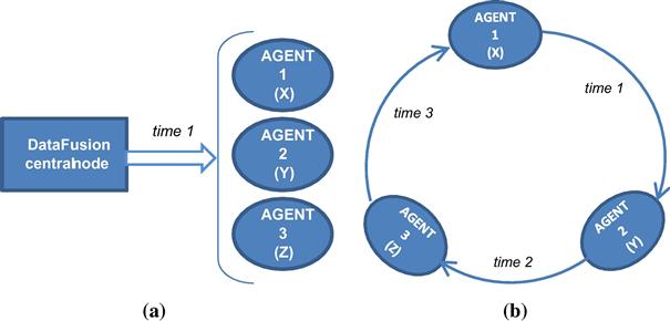
Figure 22.10 (a) centralized data fusion process model; (b) network centric data fusion process model.
The method of the centralized steepest descent applied to the function ![]() , given a starting point
, given a starting point ![]() , is based on the following iterations:
, is based on the following iterations:
 (22.2)
where ![]() , and
, and ![]() represents the step employed in the steepest descent method.
represents the step employed in the steepest descent method.
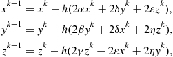
A network centric steepest descent method can be derived by the communication scheme represented in Figure 22.10b and described below. Given the starting point ![]() , the following iterations can be done:
, the following iterations can be done:
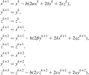 (22.3)
where ![]() and
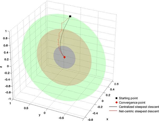
and ![]() represents the step employed in the steepest descent method. Figure 22.11 shows the comparison of the two methods for the previous model. Note that the three agents in the net-centric approach are those looking at the function to be minimized along the x, y, and z axes respectively. The black square and the red diamond in the curves represent respectively the starting point of the iteration and the final position. The black solid line shows the trajectory described by the variables
represents the step employed in the steepest descent method. Figure 22.11 shows the comparison of the two methods for the previous model. Note that the three agents in the net-centric approach are those looking at the function to be minimized along the x, y, and z axes respectively. The black square and the red diamond in the curves represent respectively the starting point of the iteration and the final position. The black solid line shows the trajectory described by the variables ![]() obtained by the application of the centralized steepest descent method; the red solid line shows the behavior of the variables obtained by the net-centric steepest descent method. Note that the red line approaches the minimum by moving along the x, y, and z axes separately. The ellipsoids of Figure 22.11 represent the iso-level surfaces of the objective function. Notice that the telecommunication network modeled for the net-centric steepest descent determines the usual Jacobi iteration employed for the solution of linear systems associated to minimization problems [94–96]. In the following Section 2.22.6.1 this approach is applied to reach the optimal deployment of a sensor network.
obtained by the application of the centralized steepest descent method; the red solid line shows the behavior of the variables obtained by the net-centric steepest descent method. Note that the red line approaches the minimum by moving along the x, y, and z axes separately. The ellipsoids of Figure 22.11 represent the iso-level surfaces of the objective function. Notice that the telecommunication network modeled for the net-centric steepest descent determines the usual Jacobi iteration employed for the solution of linear systems associated to minimization problems [94–96]. In the following Section 2.22.6.1 this approach is applied to reach the optimal deployment of a sensor network.
2.22.6 Real study cases: novel approaches to sensor networks
This section proposes several study cases of sensor networks employing novel approaches. Section 2.22.6.1 proposes an optimization method, projected in the network centric frame, to obtain the optimal deployment of a cooperative sensor network; Section 2.22.6.2 describes how to employ the so-called bio-inspired models of dynamic sensor collaboration in a chemical sensor network to detect a chemical pollutant; finally Section 2.22.6.3 gives a description of the typical problem of detection of radioactive sources.
2.22.6.1 A cooperative sensor network: optimal deployment and functioning
This section presents a mathematical model for the deployment of a sensor network, for the creation of consensus values from the noisy data measured and a statistical methodology to detect local anomalies in these data. A local anomaly in the data is associated to the presence of an intruder. The model of sensor network presented here is characterized by the absence of a fusion center. In other words the deployment, the construction of the consensus values, and the detection of local anomalies in the data are the result of local interactions between sensors. Nevertheless the local interactions will lead to global solution of the considered problem. This is an example of model of a network centric sensor network. The sensors are assumed to be identical and they measure a quantity pertinent to the properties of the area to survey able to reveal the presence of an intruder. In the proposed study case the sensors are able to measure the temperature of the territory in the position or in the “area” where they are located; in absence of anomalies there is a uniform temperature on the territory where the sensors are deployed. The sensor measures are noisy and can be considered synchronous. This measurement process is repeated periodically in time with a given frequency. From these measures a “consensus” temperature is deduced, pertinently to the territory where the sensors are deployed and an estimate of the magnitude of the noise contained in the data. Finally using these consensus values as reference values local anomalies are detected by the individual sensors. In the following we give some analytical details of the consensus method [97].
Let ![]() be a bounded connected polygonal domain in two dimensional real Euclidean space R2. The domain
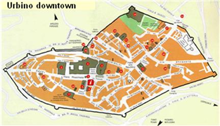
be a bounded connected polygonal domain in two dimensional real Euclidean space R2. The domain ![]() represents the territory where the sensor network must be deployed; in our case the downtown part of the Italian city of Urbino, shown in Figure 22.12. Let
represents the territory where the sensor network must be deployed; in our case the downtown part of the Italian city of Urbino, shown in Figure 22.12. Let ![]() denote the Euclidean norm of in R2. Consider N sensors
denote the Euclidean norm of in R2. Consider N sensors ![]() , located respectively, in the points
, located respectively, in the points ![]() , assumed to be distinct. To the sensor network deployed in the points
, assumed to be distinct. To the sensor network deployed in the points ![]() corresponds a graph whose nodes are the sensors location and whose edges join the sensors able to communicate between themselves. This graph is assumed to be connected and can be imagined as laid on the territory. The assumption that the graph is connected is equivalent to assuming that the sensors constitute a network. For
corresponds a graph whose nodes are the sensors location and whose edges join the sensors able to communicate between themselves. This graph is assumed to be connected and can be imagined as laid on the territory. The assumption that the graph is connected is equivalent to assuming that the sensors constitute a network. For ![]() , a polygonal region
, a polygonal region ![]() is associated to each sensor
is associated to each sensor ![]() ; this region is defined by the condition that the points belonging to
; this region is defined by the condition that the points belonging to ![]() are closest to the sensor
are closest to the sensor ![]() , that is they are closest to
, that is they are closest to ![]() , than to any other of the remaining sensors
, than to any other of the remaining sensors ![]() located in
located in ![]() . It follows:
. It follows:
![]() (22.4)
(22.4)
When for a given ![]() the minimizer of the function
the minimizer of the function ![]() is not unique we attribute
is not unique we attribute ![]() to
to ![]() , where i is the smallest index between the indices that are minimizers of the function f.
, where i is the smallest index between the indices that are minimizers of the function f.
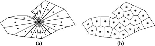
The collection of subsets ![]() defined in Eq. (22.4) and further specified by the condition above is a partition of
defined in Eq. (22.4) and further specified by the condition above is a partition of ![]() and it is a Voronoi partition of
and it is a Voronoi partition of ![]() associated to the Voronoi centers
associated to the Voronoi centers ![]() , as represented in Figure 22.13 [98], where the sets
, as represented in Figure 22.13 [98], where the sets ![]() are the Voronoi cells. The sensor
are the Voronoi cells. The sensor ![]() is located in
is located in ![]() , with
, with ![]() , and monitors the sub-region
, and monitors the sub-region ![]() of
of ![]() . Note that there is a Voronoi partition of
. Note that there is a Voronoi partition of ![]() associated to each choice of the Voronoi centers
associated to each choice of the Voronoi centers ![]() , that, completed with the graph that defines the communication between the sensors, constitute a deployment of the sensors
, that, completed with the graph that defines the communication between the sensors, constitute a deployment of the sensors ![]() on the territory
on the territory ![]() .
.
After the definition of a Voronoi partition of ![]() , we want to determine the optimal one with respect to a pre-specified criterion, that in this study case is the fact that the Voronoi centers
, we want to determine the optimal one with respect to a pre-specified criterion, that in this study case is the fact that the Voronoi centers ![]() should coincide (as much as possible) with the centers of mass of the corresponding Voronoi cells
should coincide (as much as possible) with the centers of mass of the corresponding Voronoi cells ![]() . This property translates in mathematical terms the request that the sensors are well distributed on the territory. That is what is called optimal Voronoi partition, i.e., the Voronoi partition associated to the Voronoi centers whose coordinates
. This property translates in mathematical terms the request that the sensors are well distributed on the territory. That is what is called optimal Voronoi partition, i.e., the Voronoi partition associated to the Voronoi centers whose coordinates ![]() are the solution of the following problem:
are the solution of the following problem:
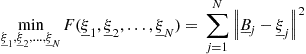 (22.5)
subject to the constraints:
![]() (22.6)
(22.6)
where ![]() is the center of mass of the Voronoi cell
is the center of mass of the Voronoi cell ![]() . Moreover we require:
. Moreover we require:
![]() (22.7)
(22.7)
That is the Voronoi centers and the centers of mass of the Voronoi cells coincide. Note that in general ![]() depends on
depends on ![]() and that the function
and that the function ![]() is in general a non linear function of
is in general a non linear function of ![]() . The solution of the problem expressed in Eqs. (22.5)–(22.7) after having specified the communications between the sensors is the optimal deployment, represented in Figures 22.13b and 22.14. When the condition of Eq. (22.7) cannot be satisfied, we may accept the available solution of Eqs. (22.5) and (22.6) as location of the Voronoi centers corresponding to the optimal deployment. Note that in general the solution of problem expressed in Eqs. (22.5)–(22.7) is not unique and it can be solved by the application of the steepest descent concept, revised in a network centric frame as shown conceptually in Section 2.22.5.7 [94]. This method can be used to solve the problem of Eq. (22.5) with an iterative procedure, that beginning from an initial guess, updates at every iteration the current approximation of the solution with a step in the direction of the gradient of the function
. The solution of the problem expressed in Eqs. (22.5)–(22.7) after having specified the communications between the sensors is the optimal deployment, represented in Figures 22.13b and 22.14. When the condition of Eq. (22.7) cannot be satisfied, we may accept the available solution of Eqs. (22.5) and (22.6) as location of the Voronoi centers corresponding to the optimal deployment. Note that in general the solution of problem expressed in Eqs. (22.5)–(22.7) is not unique and it can be solved by the application of the steepest descent concept, revised in a network centric frame as shown conceptually in Section 2.22.5.7 [94]. This method can be used to solve the problem of Eq. (22.5) with an iterative procedure, that beginning from an initial guess, updates at every iteration the current approximation of the solution with a step in the direction of the gradient of the function ![]() . Moreover the steepest descent method must be adapted to the presence of the constraints of Eq. (22.6), of the condition of Eq. (22.7) and to the requirement that its implementation must lead to a network centric solution of the deployment problem. For sake of brevity, how to impose Eq. (22.6) will not be discussed here, however a treatment of constraints in the continuous analog of the steepest descent algorithm can be found in [99]. Note also that the solutions of Eqs. (22.5) and (22.6) that are of interest are usually interior points of the constraints (6). That is the constraint issue usually is not relevant in the solution of Eqs. (22.5) and (22.6). Similarly we will not pay attention to condition of Eq. (22.7). In fact with respect to Eq. (22.7), we will simply verify if the solution of the optimization problem determined by the steepest descent method satisfies Eq. (22.7). Let us concentrate our attention on the issue of building a network centric implementation of the continuous analog of the steepest descent method to solve Eq. (22.5). Assume that the sensor
. Moreover the steepest descent method must be adapted to the presence of the constraints of Eq. (22.6), of the condition of Eq. (22.7) and to the requirement that its implementation must lead to a network centric solution of the deployment problem. For sake of brevity, how to impose Eq. (22.6) will not be discussed here, however a treatment of constraints in the continuous analog of the steepest descent algorithm can be found in [99]. Note also that the solutions of Eqs. (22.5) and (22.6) that are of interest are usually interior points of the constraints (6). That is the constraint issue usually is not relevant in the solution of Eqs. (22.5) and (22.6). Similarly we will not pay attention to condition of Eq. (22.7). In fact with respect to Eq. (22.7), we will simply verify if the solution of the optimization problem determined by the steepest descent method satisfies Eq. (22.7). Let us concentrate our attention on the issue of building a network centric implementation of the continuous analog of the steepest descent method to solve Eq. (22.5). Assume that the sensor ![]() knows only the position of its neighbor sensors, that is of the sensors that belong to a disk with center
knows only the position of its neighbor sensors, that is of the sensors that belong to a disk with center ![]() and radius
and radius ![]() . Later we will show how to choose r. The solution of the optimization problem of Eq. (22.5) is found approximating the solution of the system of differential equations:
. Later we will show how to choose r. The solution of the optimization problem of Eq. (22.5) is found approximating the solution of the system of differential equations:
![]() (22.8)
(22.8)
where ![]() denotes a real parameter, with the solution of the “network centric” system differential equations:
denotes a real parameter, with the solution of the “network centric” system differential equations:
![]() (22.9)
(22.9)
with
![]() (22.10)
(22.10)
where
![]() (22.11)
(22.11)
and ![]() being the center of mass of the Voronoi cell
being the center of mass of the Voronoi cell ![]() obtained computing the Voronoi partition of
obtained computing the Voronoi partition of ![]() associated to the Voronoi centers
associated to the Voronoi centers ![]() . Assume that
. Assume that ![]() is large enough to guarantee that
is large enough to guarantee that ![]() is neighbor of
is neighbor of ![]() when the distance between
when the distance between ![]() and
and ![]() is zero,
is zero, ![]() . Note that with this assumption we have
. Note that with this assumption we have ![]() . In Eqs. (22.8) and (22.9) the dot denotes the differentiation with respect to
. In Eqs. (22.8) and (22.9) the dot denotes the differentiation with respect to ![]() . We observe that Eq. (22.8) is known as the steepest descent differential equation. The continuous analog of the steepest descent method consists in obtaining the solution of the optimization problem of Eq. (22.5) computing the asymptotic value as
. We observe that Eq. (22.8) is known as the steepest descent differential equation. The continuous analog of the steepest descent method consists in obtaining the solution of the optimization problem of Eq. (22.5) computing the asymptotic value as ![]() goes to infinity of a solution of Eq. (22.8) equipped when
goes to infinity of a solution of Eq. (22.8) equipped when ![]() with a suitable initial condition. This asymptotic value hopefully is a point that solves Eq. (22.5) and satisfies Eqs. (22.6) and (22.7).
with a suitable initial condition. This asymptotic value hopefully is a point that solves Eq. (22.5) and satisfies Eqs. (22.6) and (22.7).
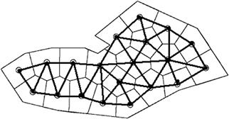
Figure 22.14 Graph associated to the optimal Voronoi partition of ![]() shown in Figure 22.13b.
shown in Figure 22.13b.
Note that the function ![]() depends only on
depends only on ![]() , that is can be computed in the location
, that is can be computed in the location ![]() using only information available in
using only information available in ![]() . Approximating the gradient of F with the appropriate pieces of the gradients of the function
. Approximating the gradient of F with the appropriate pieces of the gradients of the function ![]() , and using Eq. (22.9) instead than Eq. (22.8) we can find an approximation of the solution of Eq. (22.5) integrating numerically the initial value problem for Eq. (22.9). Note that the solution for the ith differential equation of Eq. (22.9) is computed in the location
, and using Eq. (22.9) instead than Eq. (22.8) we can find an approximation of the solution of Eq. (22.5) integrating numerically the initial value problem for Eq. (22.9). Note that the solution for the ith differential equation of Eq. (22.9) is computed in the location ![]() . This approximation of the solution of Eq. (22.5) is obtained using only local information so that it is “network centric.” When the asymptotic value as
. This approximation of the solution of Eq. (22.5) is obtained using only local information so that it is “network centric.” When the asymptotic value as ![]() goes to infinity, the solution of Eq. (22.9) coincides with an asymptotic value of a solution of Eq. (22.8), solving numerically Eq. (22.9), we can obtain in a network centric manner a solution of Eq. (22.5). The choices of the optimal Voronoi partition and of the steepest descent method to determine it, are only one of the many other legitimate choices. In Figure 22.13 the polygonal region shown represents
goes to infinity, the solution of Eq. (22.9) coincides with an asymptotic value of a solution of Eq. (22.8), solving numerically Eq. (22.9), we can obtain in a network centric manner a solution of Eq. (22.5). The choices of the optimal Voronoi partition and of the steepest descent method to determine it, are only one of the many other legitimate choices. In Figure 22.13 the polygonal region shown represents ![]() , for N = 20 and for
, for N = 20 and for ![]() , denoting with the full circle the position of the center of mass
, denoting with the full circle the position of the center of mass ![]() of the subset
of the subset ![]() and with the empty circle the position of the sensors
and with the empty circle the position of the sensors ![]() . The Figure 22.13a shows the Voronoi partition of the domain
. The Figure 22.13a shows the Voronoi partition of the domain ![]() , associated to 20 Voronoi centers
, associated to 20 Voronoi centers ![]() and the corresponding centers of mass
and the corresponding centers of mass ![]() of the associated Voronoi cells
of the associated Voronoi cells ![]() . Note that in Figure 22.13a we have
. Note that in Figure 22.13a we have ![]() . The Figure 22.13b shows an optimal Voronoi partition. Note that in Figure 22.13b we have
. The Figure 22.13b shows an optimal Voronoi partition. Note that in Figure 22.13b we have ![]() . The Voronoi partition shown in Figure 22.13b satisfies Eqs. (22.5)–(22.7). The centers of Figure 22.13b have been obtained integrating numerically, using the explicit Euler method in Eq. (22.9), equipped with the initial condition given by the centers shown in Figure 22.13a. In Figure 22.14 we show the graph associated to the optimal Voronoi partition of
. The Voronoi partition shown in Figure 22.13b satisfies Eqs. (22.5)–(22.7). The centers of Figure 22.13b have been obtained integrating numerically, using the explicit Euler method in Eq. (22.9), equipped with the initial condition given by the centers shown in Figure 22.13a. In Figure 22.14 we show the graph associated to the optimal Voronoi partition of ![]() shown in Figure 22.13b. The graph is obtained joining with branches the Voronoi centers that are (distinct) neighbors. In Figures 22.13 and 22.14 we have chosen
shown in Figure 22.13b. The graph is obtained joining with branches the Voronoi centers that are (distinct) neighbors. In Figures 22.13 and 22.14 we have chosen ![]() , where k is a parameter that can be changed during the optimization procedure used to solve Eqs. (22.5)–(22.7).
, where k is a parameter that can be changed during the optimization procedure used to solve Eqs. (22.5)–(22.7).
Remind that we have assumed that the graph G associated to the optimal deployment is connected (see Figures 22.14 and 22.13b). Moreover we remind that, since there is not a fusion center, each node of the graph G does not know the positions of all the remaining nodes of the graph, in fact it knows only the positions of its neighbor nodes. Let L be the Laplacian matrix associated to G [100]. The matrix L is a symmetric positive semi-definite ![]() matrix. Let
matrix. Let ![]() , be a real N dimensional vector depending on the real parameter
, be a real N dimensional vector depending on the real parameter ![]() . The superscript
. The superscript ![]() means transposed. We consider the system of ordinary differential equations:
means transposed. We consider the system of ordinary differential equations:
![]() (22.12)
(22.12)
equipped with the initial conditions:
![]() (22.13)
(22.13)
where ![]() denotes the usual matrix vector multiplication,
denotes the usual matrix vector multiplication, ![]() is a known initial condition and the dot denotes differentiation with respect to
is a known initial condition and the dot denotes differentiation with respect to ![]() . Since G is connected we have:
. Since G is connected we have:
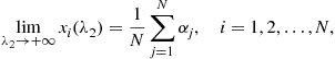 (22.14)
where ![]() , is the solution of Eqs. (22.12) and (22.13). This result follows easily from the spectral properties of L [100]. Note also that the right hand side of Eq. (22.14) is the “average” of the initial condition
, is the solution of Eqs. (22.12) and (22.13). This result follows easily from the spectral properties of L [100]. Note also that the right hand side of Eq. (22.14) is the “average” of the initial condition ![]() . Note that Eq. (22.12) can be interpreted as the “heat equation” on the graph G, that the problem of Eqs. (22.12) and (22.13) can be seen as an initial value problem for the heat equation on G and that Eq. (22.14) can be understood as the approach to an asymptotic equilibrium “temperature” in an “heat transfer” problem. We assume that during the monitoring phase the sensor measures a physical quantity, such as, for example, the temperature, of the region
. Note that Eq. (22.12) can be interpreted as the “heat equation” on the graph G, that the problem of Eqs. (22.12) and (22.13) can be seen as an initial value problem for the heat equation on G and that Eq. (22.14) can be understood as the approach to an asymptotic equilibrium “temperature” in an “heat transfer” problem. We assume that during the monitoring phase the sensor measures a physical quantity, such as, for example, the temperature, of the region ![]() where it is located. The sensors are identical, the measures made by the sensors are synchronous, repeated periodically in time and of course they are noisy. Moreover they are assumed to be independent. A first set of measures is taken by the sensors at time
where it is located. The sensors are identical, the measures made by the sensors are synchronous, repeated periodically in time and of course they are noisy. Moreover they are assumed to be independent. A first set of measures is taken by the sensors at time ![]() and is collected in the vector
and is collected in the vector ![]() , where
, where ![]() is the measure done by the sensor
is the measure done by the sensor ![]() . The set of measure
. The set of measure ![]() will be used to obtain the “consensus” value
will be used to obtain the “consensus” value ![]() of the quantity monitored in
of the quantity monitored in ![]() at time
at time ![]() . We choose:
. We choose:
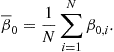 (22.15)
Remind that the sensor ![]() located in
located in ![]() knows
knows ![]() and communicates with the sensors
and communicates with the sensors ![]() located in
located in ![]() . In order to provide to the sensor
. In order to provide to the sensor ![]() , the consensus value
, the consensus value ![]() in a network centric manner we proceed as follow: we choose
in a network centric manner we proceed as follow: we choose ![]() in Eq. (22.13) and we integrate numerically the initial value problem of Eqs. (22.12) and (22.13) using the explicit Euler method to obtain a numerical approximation of
in Eq. (22.13) and we integrate numerically the initial value problem of Eqs. (22.12) and (22.13) using the explicit Euler method to obtain a numerical approximation of ![]() . Note that the ith differential equation of Eq. (22.12) is integrated in the location
. Note that the ith differential equation of Eq. (22.12) is integrated in the location ![]() , and that using the explicit Euler method this can be done using only information available in the location
, and that using the explicit Euler method this can be done using only information available in the location ![]() . Note that the analytic solution of Eqs. (22.12) and (22.13) is not “network centric” but its approximation with the explicit Euler method is “network centric.” In the former case to achieve the solution each node should know the whole graph, i.e., all the nodes. The ith node is not able to achieve the solution exploiting only the information in its posses: in this sense the solution is not “network centric.” Otherwise, exploiting the Euler approximation of the exponential of a matrix, the whole knowledge of the graph is not necessary: in this sense a “network centric” solution is achieved.
. Note that the analytic solution of Eqs. (22.12) and (22.13) is not “network centric” but its approximation with the explicit Euler method is “network centric.” In the former case to achieve the solution each node should know the whole graph, i.e., all the nodes. The ith node is not able to achieve the solution exploiting only the information in its posses: in this sense the solution is not “network centric.” Otherwise, exploiting the Euler approximation of the exponential of a matrix, the whole knowledge of the graph is not necessary: in this sense a “network centric” solution is achieved.
Once obtained ![]() we consider the following vector:
we consider the following vector:
![]() (22.16)
(22.16)
Then we choose ![]() in Eq. (22.13) and we integrate Eqs. (22.12) and (22.13) with the explicit Euler method as done above. In this way we obtain asymptotically a numerical approximation of
in Eq. (22.13) and we integrate Eqs. (22.12) and (22.13) with the explicit Euler method as done above. In this way we obtain asymptotically a numerical approximation of ![]() where:
where:
 (22.17)
This approximation of ![]() is provided to each sensor in a network centric manner. Note that
is provided to each sensor in a network centric manner. Note that ![]() is an estimate of the magnitude of the noise contained in the data; in fact
is an estimate of the magnitude of the noise contained in the data; in fact ![]() is the “sample” variance of the measures
is the “sample” variance of the measures ![]() made by the sensor at time
made by the sensor at time ![]() . The approximation of
. The approximation of ![]() and
and ![]() obtained integrating numerically Eqs. (22.12) and (22.13) are the consensus values. These values are “global” values (that is they depend on all the measures made by the sensor network at time
obtained integrating numerically Eqs. (22.12) and (22.13) are the consensus values. These values are “global” values (that is they depend on all the measures made by the sensor network at time ![]() and have been provided to each sensor in a network centric manner (that is using only “local” interactions between sensors).
and have been provided to each sensor in a network centric manner (that is using only “local” interactions between sensors).
The sensor ![]() repeats periodically in time the measure of the quantity of interest and after a given time interval has as its disposal a set of measures that can be compared with the consensus values
repeats periodically in time the measure of the quantity of interest and after a given time interval has as its disposal a set of measures that can be compared with the consensus values ![]() and
and ![]() to detect (local) anomalies. Let us assume that the set of measures made by the sensor
to detect (local) anomalies. Let us assume that the set of measures made by the sensor ![]() is a sample taken from a set of independent identically distributed Gaussian random variables of mean
is a sample taken from a set of independent identically distributed Gaussian random variables of mean ![]() and variance
and variance ![]() . In these hypotheses the Student t-test and the Chi-square test [101] are the elementary statistical tools that must be used to compare
. In these hypotheses the Student t-test and the Chi-square test [101] are the elementary statistical tools that must be used to compare ![]() and
and ![]() (that are unknown) to
(that are unknown) to ![]() and
and ![]() . The result of this comparison is the detection of local anomalies. A (statistical) significance is associated to the detected anomalies. The statistical tests used are based on the assumption that the measures come from a set of independent identically distributed Gaussian random variables. Note that the estimators
. The result of this comparison is the detection of local anomalies. A (statistical) significance is associated to the detected anomalies. The statistical tests used are based on the assumption that the measures come from a set of independent identically distributed Gaussian random variables. Note that the estimators ![]() and
and ![]() can be used in more general circumstances.
can be used in more general circumstances.
2.22.6.2 Modeling and performance analysis of a network of chemical sensors with dynamic collaboration
Typically the challenge in the deployment of an operational wireless sensor network (WSN) resides in establishing the balance between its operational requirements (e.g., minimal detection threshold, the size of surveillance region, detection time, the rate of false negatives, etc.) and the available resources (e.g., energy supply, number of sensors, communication range, fixed detection threshold of individual sensors, limited budget for the cost of hardware, maintenance, etc.) [102]. The issue of resource constraints is particularly important for a network of chemical sensors, because modern chemical sensors are equipped with air-sampling units (fans), which turn on when the sensor is active. Operating a fan requires a significant amount of energy as well as a frequent replacement of some consumable items (i.e., cartridges, filters). This leads to the critical requirement in the design of a WSN to reduce the active (air-sampling) time of its individual sensors.
One attractive way to achieve the described balance between the requirements and the constraints of WSN is to exploit the idea of dynamic sensor collaboration (DSC) [103,104]. The DSC implies that a sensor in the network should be invoked (or activated) only when the network will gain information by its activation [104]. For each individual sensor this information gain can be evaluated against other performance criteria of the sensor system, such as the detection delay or the detection threshold, to find an optimal solution in given circumstances. However, the DSC-based algorithms involve continuous estimation of the state of each sensor in the network and usually require extensive computer simulations [103,104]. These simulations may become unpractical as the number of sensors in the network increases. Furthermore, the simulations can provide the numerical values for optimal network parameters only for a specific scenario.
This motivates the development of another simple and analytic approach to the problem of network analysis and design. The main idea is to phenomenologically employ the so-called bio-inspired (epidemiology, population dynamics) or physics inspired (percolation and graph theory) models of DSC in the sensor network in order to describe the dynamics of collaboration as a single entity [105–110]. From a formal point of view, the equations of bio inspired models of DSC are the ones of the “mean-field” theory, meaning that instead of working with dynamic equations for each individual sensor we use only a small number of equations for the “averaged” sensor state (i.e., passive, active, faulty, etc.), regardless of the actual number of sensors in the system.
The analytic approach can lead to the valuable insights into the performance of the proposed sensor network system by providing simple analytical expressions to calculate the vital network parameters, such as the detection threshold, robustness, responsiveness and stability and their functional relationships.
The fluctuations in concentration C of the pollutant are modeled by the probability density function (pdf) with the mean ![]() as a parameter [111]:
as a parameter [111]:
![]() (22.18)
(22.18)
Here the value ![]() can be chosen to make it compliant with the theory of tracer dispersion in Kolmogorov turbulence [111], but it may vary with meteorological conditions. The parameter
can be chosen to make it compliant with the theory of tracer dispersion in Kolmogorov turbulence [111], but it may vary with meteorological conditions. The parameter ![]() , which models the tracer intermittency in the turbulent flow, can be in the range [0, 1], with
, which models the tracer intermittency in the turbulent flow, can be in the range [0, 1], with ![]() corresponding to the non-intermittent case. In general it also depends on the sensor position within a chemical plume, thus
corresponding to the non-intermittent case. In general it also depends on the sensor position within a chemical plume, thus ![]() near the plume centroid and may drop to
near the plume centroid and may drop to ![]() near the plume edge. For
near the plume edge. For ![]() , the pdf
, the pdf ![]() of Eq. (22.18) has a delta impulse in zero, meaning that the measured concentration in the presence of intermittency can be zero on some occasions. It can be easily shown that the pdf of Eq. (22.18) integrates to unity, so it is appropriately normalized.
of Eq. (22.18) has a delta impulse in zero, meaning that the measured concentration in the presence of intermittency can be zero on some occasions. It can be easily shown that the pdf of Eq. (22.18) integrates to unity, so it is appropriately normalized.
Depending on the values of parameters ![]() , Eq. (22.18) allows simulation of pollutant distributions with the different correlation structure (e.g., intermittent and strongly non-Gaussian) corresponding to the rich variety of possible regimes of turbulent mixing occurring in the ambient environment; Figure 22.15 shows two examples of the same WSN operating in two different correlation structures of the chemical tracer.
, Eq. (22.18) allows simulation of pollutant distributions with the different correlation structure (e.g., intermittent and strongly non-Gaussian) corresponding to the rich variety of possible regimes of turbulent mixing occurring in the ambient environment; Figure 22.15 shows two examples of the same WSN operating in two different correlation structures of the chemical tracer.
Figure 22.15 Examples of WSN network operating in the tracer filed with different correlation structure [117]. (reprinted with permission.)
We adopt a binary model of a chemical sensor, with reading V specified as:
 (22.19)
where ![]() is the threshold (an internal characteristic of the sensor). It can be shown [112] that the probability of detection of an individual sensor embedded in the environmental model described by Eq. (22.18) is given by:
is the threshold (an internal characteristic of the sensor). It can be shown [112] that the probability of detection of an individual sensor embedded in the environmental model described by Eq. (22.18) is given by:
![]() (22.20)
(22.20)
where
![]() (22.21)
(22.21)
is the cumulative distribution function corresponding to pdf of Eq. (22.18), see [113].
Suppose that N chemical sensors are uniformly distributed over the surveillance domain of area S and adopt the following network protocol for dynamic collaboration. Each sensor can be only in one of the two states: active and passive. The sensor can be activated only by a message it receives from another sensor. Once activated, the sensor remains in the active state during an interval of time ![]() ; then it “dies out” (becomes passive). While being in the active state, the sensor senses the environment and if the chemical tracer is detected, it broadcasts a (single) message. The broadcast capability of the sensor is characterized by its communication range
; then it “dies out” (becomes passive). While being in the active state, the sensor senses the environment and if the chemical tracer is detected, it broadcasts a (single) message. The broadcast capability of the sensor is characterized by its communication range ![]() . This network with the described dynamic collaboration can be modeled using the epidemic SIS model (susceptible-infected-susceptible) [114]:
. This network with the described dynamic collaboration can be modeled using the epidemic SIS model (susceptible-infected-susceptible) [114]:
 (22.22)
where ![]() denote the number of active and passive sensors, respectively. The nonlinear terms on the right hand side of Eq. (22.22) are responsible for the interaction between the sensors; parameter
denote the number of active and passive sensors, respectively. The nonlinear terms on the right hand side of Eq. (22.22) are responsible for the interaction between the sensors; parameter ![]() is a measure of this interaction. The number of sensor is assumed constant, hence we have an additional equation:
is a measure of this interaction. The number of sensor is assumed constant, hence we have an additional equation: ![]() . Since the parameter alpha describes the intensity of social interaction in a community [114] we can propose that:
. Since the parameter alpha describes the intensity of social interaction in a community [114] we can propose that:
![]() (22.23)
(22.23)
where m is the number of contacts made by the activated (“infected”) sensor during its infectious period ![]() (i.e., the number of sensors that received the wake-up message from an alerting sensor). In our case
(i.e., the number of sensors that received the wake-up message from an alerting sensor). In our case ![]() . Then we have:
. Then we have:
![]() (22.24)
(22.24)
where G is a calibration constant. In order to simplify notation we will further assume that G is absorbed in the definition of ![]() . Equation (22.22) combined with
. Equation (22.22) combined with ![]() can be reduced to one equation for
can be reduced to one equation for ![]() :
:
![]() (22.25)
(22.25)
where ![]() . By simple change of variables
. By simple change of variables ![]() , this equation can be reduced to the standard logistic equation [115,116]:
, this equation can be reduced to the standard logistic equation [115,116]:
![]() (22.26)
(22.26)
The solution of the logistic equation is well-known:
![]() (22.27)
(22.27)
where ![]() . Observe that the WSN will be able to detect the presence of a pollutant only if
. Observe that the WSN will be able to detect the presence of a pollutant only if ![]() , because then
, because then ![]() as
as ![]() independent of
independent of ![]() . In this case, after a certain transition interval, the WSN will reach a new steady state with:
. In this case, after a certain transition interval, the WSN will reach a new steady state with:
![]() (22.28)
(22.28)
From (22.27) and using the expression for b stated above, the activation time (transition interval) is given by:
![]() (22.29)
(22.29)
From Eq. (22.29) it follows that the key requirement for the network to be operational ![]() is that
is that ![]() , that is:
, that is:
![]() (22.30)
(22.30)
where ![]() is a well-known parameter in epidemiology, referred to as the basic reproductive number [114]. Observe that
is a well-known parameter in epidemiology, referred to as the basic reproductive number [114]. Observe that ![]() is independent of
is independent of ![]() ; however, according to Eq. (22.29) the response time of the WSN is strongly dependent on
; however, according to Eq. (22.29) the response time of the WSN is strongly dependent on ![]() .
.
It remains to specify q, the number of sensors that should initially be active for the described WSN with dynamic collaboration to be effective. The initial condition is simply ![]() , that is on average
, that is on average ![]() . Eqs. (22.28)–(22.30) are important analytic results. For a given level of mean pollutant concentration
. Eqs. (22.28)–(22.30) are important analytic results. For a given level of mean pollutant concentration ![]() and meteorological conditions (
and meteorological conditions (![]() , these expressions provide a simple yet rigorous way to estimate how a change in network and sensor parameters (i.e.,
, these expressions provide a simple yet rigorous way to estimate how a change in network and sensor parameters (i.e., ![]() will affect the network performance (i.e.,
will affect the network performance (i.e., ![]() .
.
The examples of agent-based simulation of “information epidemic” in WSN, which satisfies the threshold condition of Eq. (22.30) is presented in Figure 22.16. We can observe that by change of the configuration parameters of WSN we can vary the activation time and the saturation limit of the detection system. Further development of the theoretical framework presented in this section can be found in [117–120].
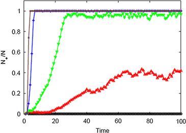
Figure 22.16 Examples of Information Epidemic in WSN of chemical sensors for different values of parameters ![]() in Eq. (22.18). (Black, blue, green and red lines correspond to
in Eq. (22.18). (Black, blue, green and red lines correspond to ![]() , respectively.) (For interpretation of the references to color in this figure legend, the reader is referred to the web version of this book.)
, respectively.) (For interpretation of the references to color in this figure legend, the reader is referred to the web version of this book.)
2.22.6.3 Detection and localization of radioactive point sources with experimental verification
Recently there has been an increased interest in detection and localization of radioactive material [121–125]. Radioactive waste material is relatively easy to obtain with numerous accidents involving its loss or theft reported. The danger is that a terrorist group may acquire some radiological material and use it to build a dirty-bomb. The dirty bomb would consist of waste by products from nuclear reactors wrapped in conventional explosives, which upon detonation would expel deadly radioactive particles into the environment. The ability to rapidly detect and localize radioactive sources is important in order to disable and isolate the potential threat in emergency situations.
This section is concerned with radiological materials that emit gamma rays. The probability that a gamma radiation detector registers ![]() counts (N being the set of natural numbers including zero) in
counts (N being the set of natural numbers including zero) in ![]() seconds, from a source that emits on average
seconds, from a source that emits on average ![]() counts per second is [126]:
counts per second is [126]:
![]() (22.31)
(22.31)
where ![]() is the mean and variance of the Poisson distribution. The measurements of radiation field are assumed to be made using a network of low-cost Geiger-Müller (GM) counters as sensors. In general, the problem of detection and localization of point sources or radioactive sources can be solved using either controllable or uncontrollable sensors. Controllable sensors can move and vary the radiation exposure time [127,128]. In this Section we will focus on uncontrollable sensors, placed at known locations with constant and known exposure times.
is the mean and variance of the Poisson distribution. The measurements of radiation field are assumed to be made using a network of low-cost Geiger-Müller (GM) counters as sensors. In general, the problem of detection and localization of point sources or radioactive sources can be solved using either controllable or uncontrollable sensors. Controllable sensors can move and vary the radiation exposure time [127,128]. In this Section we will focus on uncontrollable sensors, placed at known locations with constant and known exposure times.
Assume that ![]() sources (r is unknown) are present in the area of interest. Furthermore, the assumption is that the area is flat without obstacles (“open field”). Each source
sources (r is unknown) are present in the area of interest. Furthermore, the assumption is that the area is flat without obstacles (“open field”). Each source ![]() is parameterized by its 2D location
is parameterized by its 2D location ![]() and its equivalent strength
and its equivalent strength ![]() (a single parameter which takes into account the activity of the source, the value of gamma energy per integration and scaling factors involved, see [129]). Thus the parameter vector of source i is
(a single parameter which takes into account the activity of the source, the value of gamma energy per integration and scaling factors involved, see [129]). Thus the parameter vector of source i is ![]() , while the total parameter vector is a stacked vector:
, while the total parameter vector is a stacked vector: ![]() . Suppose a network of GM counters is deployed in the field of interest. Let GM counter
. Suppose a network of GM counters is deployed in the field of interest. Let GM counter ![]() , located at
, located at ![]() , reports its count
, reports its count ![]() every
every ![]() seconds. Assuming that each GM counter has a uniform directional response and that attenuation of gamma radiation due to air can be neglected, the joint density of the measurement vector
seconds. Assuming that each GM counter has a uniform directional response and that attenuation of gamma radiation due to air can be neglected, the joint density of the measurement vector ![]() , conditional on the parameter vector
, conditional on the parameter vector ![]() and the knowledge that r sources are present, can be modeled as [129]:
and the knowledge that r sources are present, can be modeled as [129]:
 (22.32)
Here ![]() is the mean radiation count at sensor j:
is the mean radiation count at sensor j:
 (22.33)
with
![]() (22.34)
(22.34)
being the distance between the source i and sensor j, and ![]() the average count due to the background radiation (assumed known). The problem for the network of GM counters is to estimate the number of sources r and the parameter vector for each source
the average count due to the background radiation (assumed known). The problem for the network of GM counters is to estimate the number of sources r and the parameter vector for each source ![]() . In this section we will present the experimental results obtained using real data and a Bayesian estimation algorithm combined with the minimum description length (MDL) for source number estimation.
. In this section we will present the experimental results obtained using real data and a Bayesian estimation algorithm combined with the minimum description length (MDL) for source number estimation.
A radiological field trial was conducted on a large, flat, and open area without any obstacles at the Puckapunyal airfield site in Victoria, Australia. The measurements were collected using the DSTOs3 Low Cost Advanced Airborne Radiological Survey (LCAARS) survey system which consists of an AN/PDR-77 radiation survey meter equipped with an RS232 interface module, a gamma probe and software written in Visual Basic running on a laptop computer. The gamma probe contains two GM tubes to cover both low and high ranges of dose rates. It was capable of measuring gamma radiation dose rates from background to 9.99 Sv/h4 without saturating [130] with a fairly flat response [131]. Three radiation sources were used in the field trial: source 1 was a cesium sources ![]() with
with ![]() , source 2 was also a cesium source with
, source 2 was also a cesium source with ![]() , and source 3 was a cobalt source
, and source 3 was a cobalt source ![]() with
with ![]() . The aerial image of the experimental site with the location of sources and the local Cartesian coordinate system is shown in Figure 22.17. Four data sets were collected during the field trails in the presence of r sources, with respectively
. The aerial image of the experimental site with the location of sources and the local Cartesian coordinate system is shown in Figure 22.17. Four data sets were collected during the field trails in the presence of r sources, with respectively ![]() [132]. Data sets with
[132]. Data sets with ![]() sources contains 50 count measurements in each measurement point.
sources contains 50 count measurements in each measurement point.
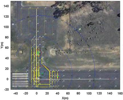
Figure 22.17 Aerial image of the experimental site with the local coordinate system. (green points indicate the locations of three sources; red circles indicate the zones with dangerous levels of radiation.) (For interpretation of the references to color in this figure legend, the reader is referred to the web version of this book.)
Estimation of parameter vector ![]() , under the assumption that r is known, was carried out using the Bayesian importance sampling technique known as the progressive correction [125,133]. This technique assumes that prior distribution of
, under the assumption that r is known, was carried out using the Bayesian importance sampling technique known as the progressive correction [125,133]. This technique assumes that prior distribution of ![]() , denoted
, denoted ![]() , is available. The information contained in the measurement vector
, is available. The information contained in the measurement vector ![]() is combined with the prior to give the posterior pdf:
is combined with the prior to give the posterior pdf: ![]() . The minimum mean squared error estimate of
. The minimum mean squared error estimate of ![]() is then the posterior expectation:
is then the posterior expectation:
![]() (22.35)
(22.35)
The problem is that the posterior pdf and hence the posterior expectation of Eq. (22.35) cannot be found analytically for the described problem. Instead, an approximation of Eq. (22.35) is computed via the importance sampling: it involves drawing ![]() samples of the parameter vector from an importance density and approximating the integral by a weighted sum of the samples. This is carried out in a few stages, each stage drawing samples from a “target distribution” which is gradually approaching the true posterior. The “target distribution” at stage
samples of the parameter vector from an importance density and approximating the integral by a weighted sum of the samples. This is carried out in a few stages, each stage drawing samples from a “target distribution” which is gradually approaching the true posterior. The “target distribution” at stage ![]() is constructed as:
is constructed as:
![]() (22.36)
(22.36)
where ![]() with
with ![]() and
and ![]() . An adaptive scheme for the computation of S and factors
. An adaptive scheme for the computation of S and factors ![]() is given in [125,133]. Assume that a random sample
is given in [125,133]. Assume that a random sample ![]() from
from ![]() is available and one wants to generate the samples or particles from
is available and one wants to generate the samples or particles from ![]() . The progressive correction algorithm steps are then as follows [125]:
. The progressive correction algorithm steps are then as follows [125]:
2. compute not-normalized weight of each sample as: ![]() , for
, for ![]() ;
;
4. perform re-sampling of particles [134];
5. carry out Markov chain Monte Carlo (MCMC) move step for each particle [134].
The procedure is repeated for every stage ![]() until
until ![]() . The initial set of particles is drawn from the prior density
. The initial set of particles is drawn from the prior density ![]() . The final estimate in Eq. (22.35) is approximated as
. The final estimate in Eq. (22.35) is approximated as
 (22.37)
The number of sources was estimated using the MDL algorithm [59], which will choose ![]() that will maximize the following quantity:
that will maximize the following quantity:
![]() (22.38)
(22.38)
where ![]() is the estimate obtained under the assumption that r sources are present and
is the estimate obtained under the assumption that r sources are present and
![]() (22.39)
(22.39)
is the Fisher Information Matrix. It can be shown that
 (22.40)
with
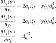 (22.41)
The inverse of the FIM gives us the CRLB, which represents the theoretical lower bound for estimation error covariance [135]. Figure 22.18 shows the output of the progressive correction algorithm for data set 3 (with three sources present) after (a) ![]() and (b)
and (b) ![]() stages of processing. The red stars indicate the locations of three sources. The green line shows the initial polygon A for the location of sources. The prior density for sampling the initial set of particles for source
stages of processing. The red stars indicate the locations of three sources. The green line shows the initial polygon A for the location of sources. The prior density for sampling the initial set of particles for source ![]() is:
is:
![]() (22.42)
(22.42)
where ![]() stands for uniform distribution over the polygon A and
stands for uniform distribution over the polygon A and ![]() is the gamma distribution with parameters
is the gamma distribution with parameters ![]() and
and ![]() . From Figure 22.18 we observe how the progressive correction algorithm localiszs the three sources fairly accurately.
. From Figure 22.18 we observe how the progressive correction algorithm localiszs the three sources fairly accurately.
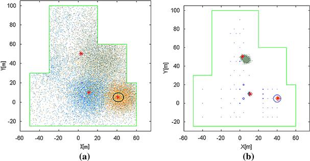
Figure 22.18 The output of progressive correction algorithm after (a) ![]() and (b)
and (b) ![]() stages: data set 3 with
stages: data set 3 with ![]() sources present (indicated by red stars). (For interpretation of the references to color in this figure legend, the reader is referred to the web version of this book.)
sources present (indicated by red stars). (For interpretation of the references to color in this figure legend, the reader is referred to the web version of this book.)
As we mentioned earlier, 50 count measurements have been collected by each sensor. This allows us to find the root mean square (rms) estimation error using each snapshot of measurement data from all sensors. Table 22.2 shows the resulting rms errors versus the theoretical CRLB.
Table 22.2
RMS Error of Progressive Correction Algorithm Versus the Theoretical Bound for Data Set 3 (![]() )
)
The theoretical CRLB was computed using the idealized measurement model as stated by Eqs. (22.32)–(22.34). Considering that this measurement model was very crude with a number of factors neglected (e.g., uniform directional response, neglected air attenuation, perfect knowledge of sensor locations, known and constant average background radiation, etc.), the agreement between the theoretical bound and the RMS estimation errors in Table 22.2 is remarkable. The experimental results in this table effectively verify the measurement model as well as the estimation algorithm.
Results for estimation of r are shown in Table 22.3. The table lists the number of runs (out of 50) that resulted in ![]() . It can be observed that the number of sources is estimated correctly in the majority of cases.
. It can be observed that the number of sources is estimated correctly in the majority of cases.
Table 22.3
Estimation of the Number of Sources Using the Progressive Correction in the MDL Algorithm

More results of experimental data processing can be found in [131,132]. In a recent study [136] it was found that by using all 50 snapshots of measurement data for estimation by progressive correction, results in a posterior pdf which is very narrow but does not include the true source positions. This indicates that the measurement model is not perfect, which is not surprising considering that it is based on many approximations. In situations where the measurement likelihood is not exact, it is necessary to introduce a degree of caution to make the estimation more robust. In the framework of progressive correction this can be achieved by ![]() . In this way the measurement likelihood is effectively approximated by a fuzzy membership function which has a theoretical justification in random set theory [137, Chapter 7].
. In this way the measurement likelihood is effectively approximated by a fuzzy membership function which has a theoretical justification in random set theory [137, Chapter 7].
If one wants to relax the assumption that radioactive sources are point sources, the problem becomes the one of radiation field estimation. This is an inverse problem, difficult to solve in general. By modeling the radiation field by a Gaussian mixture, however, the problem becomes tractable and some recent results are reported in [138].
2.22.7 Heterogeneous multi-sensor network management
Multi-sensor management concerns with the control of environment perception activities by managing or coordinating the usage of multiple heterogeneous sensor resources. Multi-sensor systems are becoming increasingly important in a variety of military and civilian applications. Since a single sensor generally can only perceive limited partial information about the environment, multiple similar and/or dissimilar sensors are required to provide sufficient local pictures with different focus and from different viewpoints in an integrated manner. As viewed, information from heterogeneous sensors can be combined using data fusion algorithms to obtain synergistic observation effects. Thus the benefit of multi-sensors system are to broaden perception and enhance awareness of the state of the world compared to what could be acquired by a single sensor system. The increased sophistication of sensor assets along with the large amounts of data to be processed has pushed the information acquisition problem far beyond what can be handled by human operator. This motivates the emerging interest in research into automatic and semi-automatic management of sensor resources for improving overall perception performance beyond basic fusion of data.
Multi-sensor management is formally described as a system or process that seeks to manage or coordinate the usage of a suite of sensors or measurement devices in a dynamic, uncertain environment, to improve the performance of data fusion and ultimately that of perception.
The basic objective of sensor management is to select the right sensors to do the right service on the right object at the right time. Sensor management, aiming at improving data fusion performance by controlling sensor behavior, plays the role of level 4 functions in JDL model presented in Section 2.22.3. Mainly the same considerations made for homogeneous sensor networks are still valid: the criteria followed to manage the network remains the same, however there is an increasing of complexity due to the diversity of the sensors. In the following Sections the problems related to multi-sensor management are divided into three main categories i.e., sensor deployment, sensor behavior assignment, and sensor coordination.
2.22.7.1 Sensor deployment
Sensor deployment is a critical issue for intelligence collection in an uncertain dynamic environment. It concerns with making decisions about when, where, and how many sensing resources need to be deployed in reaction to the state of the environment and its changes.
Sensor placement needs special attention in sensor deployment. It consists of positioning multiple sensors simultaneously in optimal or near optimal locations to support surveillance tasks when necessary. Typically it is desired to locate sensors within a particular region determined by tactical situations to optimize a certain criterion usually expressed in terms of global detection probability, quality of tracks, etc. This problem can be formulated as one of constrained optimization of a set of parameters. It is subject to constraints due to the following factors:
• sensors are usually restricted to specified regions due to tactical considerations;
• critical restrictions may be imposed on relative positions of adjacent sensors to enable their mutual communication when sensors are arranged as distributed assets in a decentralized network (e.g., net-centric approach);
• the amount of sensing resources that can be positioned in a given period is limited due to logistical restrictions.
In simple cases, decisions on sensor placement are to be made with respect to a well-prescribed and stationary environment. An example of a stationary problem is the placing of radars to minimize the terrain screening effect in detection of an aircraft approaching a fixed site. Another example is the arrangement of a network of intelligence gathering assets in a specified region to target another well-defined area. In the above scenarios, mathematical or physical models such as terrain models, propagation models, etc. are commonly available and they are used as the basis for evaluation of sensor placement decisions. Paper [139] presents a study for finding a solution to the placement of territorial resources for multi-purpose telecommunication services considering also the restrictions imposed by the orography of the territory itself. To solve this problem genetic algorithms5 are used to identify sites to place the resources for the optimal coverage of a given area. The used algorithm has demonstrated to be able to find optimal solutions in a variety of considered situations.
More challenging are those situations in which the environment is dynamic and sensors must repeatedly be repositioned to be able to refine and update the state estimation of moving targets in real time. Typical situations where reactive sensor placement is required are, for instance, submarine tracking by means of passive sonobuoys in an anti-submarine warfare scenario; locating moving transmitters using ESM (Electronic Support Measures) receivers; tracking of tanks on land by dropping passive acoustic sensors.
2.22.7.2 Sensor behavior assignment
The basic purpose of sensor management is to adapt sensor behavior to dynamic environments. By sensor behavior assignment is meant efficient determination and planning of sensor functions and usage according to changing situation awareness or mission requirements. Two crucial points are involved. Firstly the decisions about the set of observation tasks (referred to as system-level tasks) that the sensor system is supposed to accomplish currently or in the near future, on the basis of the current/predicted situation as well as the given mission goal. Secondly the planning and scheduling of actions of the deployed sensors to best accomplish the proposed observation tasks and their objectives.
Owing to limited sensing resources, it is prevalent in real applications that available sensors are not able to serve all desired tasks and achieve all their associated objectives simultaneously. Therefore a reasonable compromise between conflicting demands is sought. Intuitively, more urgent or important tasks should be given higher priority in their competition for resources. Thus a scheme is required to prioritize observation tasks. Information about task priority can be very useful in scheduling of sensor actions and for negotiation between sensors in a decentralized paradigm.
To focus on this class of problems, let us consider a scenario including a number of targets as well as multiple sensors, which are capable of focusing on different objects with different modes for target tracking and/or classification. The first step for the sensor management system should be to utilize evidences gathered to decide objects of interest and to prioritize which objects to look at in the time following. Subsequently, in the second step, different sensors together with their modes are allocated across the interesting objects to achieve best situation awareness. In fact, owing to the constraints on sensors and computational resources, it is in general not possible to measure all targets of interest with all sensors in a single time interval. Also, improvement of the accuracy on one object may lead to degradation of performance on another object. What is required is a suitable compromise among different targets.
2.22.7.3 Sensor coordination in a decentralized sensor network
As stated in the previous Sections, there are two general ways to integrate a set of sensors into a sensor network. One is the centra1ized paradigm, where all actions of all sensors are decided by a central mechanism. The other alternative is to treat sensors in the network as distributed intelligent agents with some degree of autonomy. In such a decentralized architecture, bi-directional communication between sensors is enabled, so that communication bottlenecks possibly existing in a centralized network can be avoided. A major research objective of decentralized sensor management is to establish cooperative behavior between sensors with no or little external supervision. In a decentralized sensor network scenario a local view perceived from a sensor can be shared by some members of the sensor community. Intuitively, a local picture from one sensor can be used to direct the attention of other sensors or transfer tasks such as target tracking from one sensor to another. An interesting question is how participating sensors can autonomously coordinate their movements and sensing actions, on grounds of shared information, to develop an optimal global awareness of the environment with parsimonious consumption of time and resources.
As for homogeneous sensor network, the CSIP approach can be exploited [141,142]: the network consists of different kinds of sensors, randomly distributed inside the surveillance area and if the number of sensors is high, the performance of the surveillance system can be considered independent of the location of the targets. Each sensor has a different functioning level. A first level sensor, with small sensing and communication capabilities may provide only detection information; a second level sensor may provide detection and localization information, with medium sensing and communication capabilities. Finally a third level sensor may provide tracking information and may be able to perform target recognition and classification. Usually the number of low level sensors exceeds the number of higher level sensors and only close sensors exchange data.
In [143] the network consists of two types of sensors: simple and complex as represented in Figure 22.19a. The simple ones have only the capability of sensing their coverage area with a reduced computation capabilities and they transmit data to complex sensors. The information they provide may be encoded, for example, by a “1” if sensor detects something crossing its coverage area and by a “0” otherwise. Complex sensors, instead, have computation capabilities; they are able to locate the target by applying sophisticated algorithms (e.g., in [143] the maximum likelihood estimation algorithm is applied). The topology simulated in [143], constituted by 80 simple sensors and 20 complex sensors, is represented in Figure 22.19b: the sensors are indicated by circles; the complex sensors are connected by the solid lines, simple and complex sensor by dashed lines. Figure 22.20 shows the number of active sensors during the target tracking: the theoretical value and the simulated value are compared. It is evident that in a self-organizing configuration the number of active sensors is optimized with the consequent advantage of saving of power.
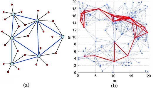
Figure 22.19 (a) Network architecture scheme; (b) deployment of simple and complex nodes simulated in [143]. (Reprinted with permission.)
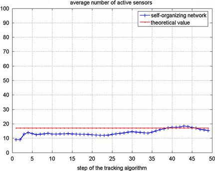
Figure 22.20 Average number of active sensors as function of the step number of the algorithm; simulation and theoretical values. (From [143], reprinted with permission.)
An adaptive self-configuring system consists of a collection of independent randomly located sensors that, carrying ahead local interactions, estimate the position of the target without a centralized control unit that coordinates their communication. It is fault tolerant and adapts to changing conditions. Furthermore, it is able to self-configuring, i.e., there is not an external entity that configures the network. Finally, the task is performed efficiently, i.e., it guarantees both a reasonably long network life and good target tracking performances. From local interactions, sensors form an efficient system that follows the target, i.e., local communication leads to a self-organizing network that exploits the features of the theories of random graphs and of self-organizing systems. The most natural way to approach random network topology is by means of the theory of random graphs [144,145]. The theory of random graphs allows, for instance, to compute an upper bound to the estimated number of active sensors at each time step.
2.22.7.4 A mathematical issue for multi-sensor networks
When the fusion of heterogeneous signals is performed, there is a formal problem to solve. The signal received by the different sensors may be statistically dependent because of the complex intermodal interactions; usually the statistical dependence is either ignored or not adequately considered. Usually the multiple hypotheses testing theory is based on the statistical independence of the received signals, in our case this condition is not maintained, therefore techniques as the “copula probability theory” may be useful.
In probability theory and statistics, a copula can be used to describe the dependence between random variables [146]. The cumulative distribution function of a random vector can be written in terms of marginal distribution functions and a copula. The marginal distribution functions describe the marginal distribution of each component of the random vector and the copula describes the dependence structure between the components. Copulas are popular in statistical applications as they allow one to easily model and estimate the distribution of random vectors by estimating marginal distributions and copula separately. The Sklar’s theorem ensures that the joint cumulative distribution function (cdf) ![]() of random variables
of random variables ![]() are joined by a copula function
are joined by a copula function ![]() to the respective marginal distributions
to the respective marginal distributions ![]() as [147]:
as [147]:
![]() (22.43)
(22.43)
Further, if the marginals are continuous, ![]() is unique. By the differentiation of the joint cdf, the joint pdf is obtained:
is unique. By the differentiation of the joint cdf, the joint pdf is obtained:
 (22.44)
The copula density ![]() , function of the N marginals from the N sensors, represents a correction term of the independent product of densities of Eq. (22.44).
, function of the N marginals from the N sensors, represents a correction term of the independent product of densities of Eq. (22.44).
Processing heterogeneous data set is not straightforward as they may not be commensurate. In addition, the signals may also exhibit statistical dependence due to overlapping fields of view. In [148] the authors propose a copula-based solution to incorporate statistical dependence between disparate sources of information. The important problem of identifying the best copula for binary classification problems is also addressed and a copula based test-statistic, able to decouples marginals and dependency information, is developed.
2.22.8 Border control problem via electronic fence
This section tackles the problem of the surveillance of the borders of a nation. The region of interest, in general, may be very wide consisting even of thousands of kilometers of coastline and land border line, and millions of square kilometers. Such a system must face threats such as drug trafficking, intrusions (man, vehicles and airplanes), illegal immigration, smuggling, human trafficking, arms smuggling, unauthorized deforestation, terrorist activities over the military defense of the borders in order to ensure the territorial defense and the national sovereignty in the areas close to the border line. In the following Sections an overview of the range of possibilities and solutions in the design of the surveillance asset and data fusion process of such systems devoted to border control is given.
2.22.8.1 Multi-scale approach
The size of the region, the nature of the border and the complexity of the scenario require the provision of different pictures of the region with different field of view at different resolution and time scales, suggesting a multi-sensor/multi-scale approach integrated in a hierarchical architecture of the whole system. Typically a global field of view of the whole region is necessary at the higher Command and Control (C2) level to capture the overall situation. A higher level of resolution and refresh rate is necessary at the lower and local level to analyze and control in depth each single zone of a region. Therefore the surveillance segment may be structured according to a multilayer architecture where layers realize different trade-offs in terms of field of view and granularity and refresh time. The surveillance segment comprises several types of sensors, each one characterized by different achievable resolution, field of view, and revisiting time. A pictorial sketch of the surveillance architecture is depicted in Figure 22.21 for a notional country: sensors on board of satellites are expected to provide a global coverage of the monitored area at medium resolution with a low refresh rate, typically in the order of several hours or days; a higher resolution data and a higher refresh rate, in the order of seconds or tens of seconds, is provided by ground sensors on limited areas; airborne sensors (e.g., Unmanned Air Vehicle, UAV) will provide data on remote areas with good resolution data and short deployment time.
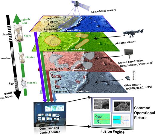
All data collected by the sensors are exploited by the fusion engine, highlighted in the figure. It is responsible to track and classify relevant entities present in the scenario and to provide a high quality representation of the situation. Also the data fusion process supports this multi-scale approach performing a distributed and network-centric processing at the various levels of the architecture, in accordance with available communication bandwidth and latency.
2.22.8.2 The electronic fence
The surveillance of critical perimeters is one of the most important issues in Homeland defense and Homeland Protection systems. The ground surveillance needs are relevant to border protection applications, but include also local area protection, such as critical infrastructure, military/civilian posts.
During the last 10 years special attention has been focused on the realization of so-called “electronic fence” for perimeter/border control and several developments have been carried out to demonstrate the efficiency of such systems. However several problems occurred when the electronic fences became operational, showing lacks in the practical use by the operators (i.e., high number of false alarms, loss of/slow communication links) together with the problem of the high funding required for the whole system. One example is described in [149], that requires now a total different approach for the surveillance of a wide national border (![]() ).
).
In the following an overview of the problems and solutions related to the implementation of an electronic fence is presented. The major components are:
• Sensors: they may be either active or passive, radar networks or heterogeneous sensor networks, (e.g., passive IR—infrared, seismic, acoustic, electro-optic—E/O, etc.).
• Communication network: necessary to data exchange, may be subdivided into sub-networks if necessary.
• Fusion engines: they perform data collection, data fusion and classification; this capability can be spread across the layers that compose the electronic fence (i.e., in the master stations, but also in the C2 centers).
Depending on the geographical deployment of the protection system, the data are then exchanged with C2 centers, both at local level and wide area (i.e., national) level. In Figure 22.22 an example of an electronic fence architecture is depicted. In this case a wide area to be controlled, such as a border of a nation, has been considered; the subnets are geographically distributed along the boundaries. The architecture has the advantage to be modular and scalable and it can be organized with different level C2 centers (local, regional, national), depending also on the size of the considered boundaries. Each subnet is able to ensure the data exchange among the sensors. An overview of the sensors that can be employed in an electronic fence is presented.
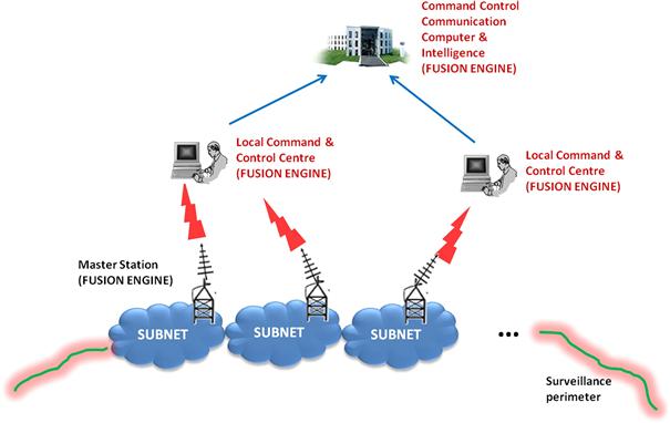
2.22.8.2.1 Sensors
Ground-based sensors
Microwave (X, Ku, Ka band) ground based radars are widely used to perform the monitoring of open wide areas. The monitoring of walking people and vehicles for ground applications, and of small sized boat for sea and river applications are relevant. The detection ranges varies from 2 km to 10 km for people, and from 5 km to 20 km for vehicles. Aerial targets (e.g., helicopters, low level aircraft) are also detected. Depending on the technology used these radars can be subdivided into the following two categories:
• Incoherent: they are low cost devices, FMCW (Frequency Modulated Continuous Wave) or pulsed (often a magnetron is used as most of the navigational radars), where the detection of the moving targets is based on inter-clutter visibility. Resolutions are typically of few meters or tenths of meters both in range and cross-range.
• Coherent: they are solid state transmitter based, FMCW or pulse compressed, where the detection of the moving targets is based on sub-clutter visibility. The MTD (Moving Target Detection) filtering, even if the radar is working at X-band, requires low scan rates (in the order of 1–3 RPM—Round Per Minute) to allow high Doppler frequency resolution (0.2–0.5 m/s) to resolve slow moving target also in presence of strong clutter [150].
Airborne sensors
The attention is for sensors able to operate in critical environments and many studies have been performed, in this direction, mainly using aerial platforms equipped with SAR. The aircraft equipped with sensors are used for wide areas where ground based sensors are not suitable or cannot be installed, such as in forest or jungle. However the use of airborne platforms to perform surveillance, are limited to missions “on spot” because it is not practical or cost/effective for continuous surveillance. The radar sensor can be mounted on manned or unmanned aircraft, usually equipped with electro-optic devices, and they can be used to monitor areas of several tenths of kilometer length. Other solutions take into account the installation of the radar either on a tethered aerostat or on a hovering helicopter. GMTI (Ground Moving Target Indication) from a stationary platform has been demonstrated.
FOliage PENetrating (FOPEN) radar
Fixed radars for border control are usually in X and Ku band, but, because of the attenuation they suffer from foliage, they cannot be used for FOPEN applications. The ability of traditional microwave radars in operating in an environment with dense foliage is severely limited by foliage backscatter and attenuation of microwave frequencies through foliage [151]. As attenuation falls with increasing wavelength, lower frequencies such as those in the VHF and UHF bands (30–1000 MHz) may be suitable for FOPEN radar applications [152–155]. FOPEN SAR (Synthetic Aperture Radar) systems started to be used in the early 1990s. They are usually mounted on manned or unmanned aircraft and mainly address illegal activity control and search-and-rescue operations. The focus is now for ground based systems and/or sensors with capabilities to detect walking personnel and moving vehicles [156]. Logistic constraints drive the technology to very low power devices, that are able to operate for several months or years, without maintenance. Another important issue is, together with a good probability of detection, the low false alarm probability, that is requested to be lowered up to 1 false alarm per day, or lower, even in presence of specific weather conditions (rain, wind) and/or local seasonal fauna.
A special attention is due to the effect of environment. In dense foliage environments the main clutter effects are the backscatter and the attenuation.
Backscatter: The fixed clutter returns can have a zero Doppler component raising up to 60–70 dB above the noise level with spectra amplitude and shape without large variations with frequency, but depending mainly on the wind strength [150]. Considering the measurements reported in [150] of the backscatter Doppler spectra, in order to perform efficient clutter rejection, two values of thresholds can be used: i.e., 1 m/s in case of light air, 2 m/s in case of windy/gale.
Attenuation: The attenuation depends mainly on the frequency used and the radar beam grazing angle, even if small variations are reported with different polarizations [153]. Many studies have been carried out for SAR application and several studies report data for attenuation measured directly at ground level [151,153,154,157]. The total attenuation, taking in account the major effects of the environment for a ground radar, can be summarized as follows:
![]() (22.45)
(22.45)
where:
• ![]() is the attenuation due to distance R,
is the attenuation due to distance R,
• ![]() is the attenuation due to the ground reflection at the heights of the antenna (
is the attenuation due to the ground reflection at the heights of the antenna (![]() and the target (
and the target (![]() , for the wavelength
, for the wavelength ![]() ,
,
• ![]() is the attenuation due to the foliage: it depends on the distance, the polarization and the forest type. It depends also on the distribution of the trees and the diameter of the masts, that can limit the line of sight, together with the height and density of lower canopy level.
is the attenuation due to the foliage: it depends on the distance, the polarization and the forest type. It depends also on the distribution of the trees and the diameter of the masts, that can limit the line of sight, together with the height and density of lower canopy level.
The main requirements/constraints addressed are the range of the detections, which is reduced by the attenuation due to foliage and the low antenna height, that is usually limited to 1–2 m for logistic purposes. Also the power consumption must be kept at minimum level, also considering that photovoltaic cells are not suitable for installation on the ground in the forest. As a consequence the emitted power must be kept at a level of several mW. Camouflage and anti-tamper are often required. Very low cost is a mandatory requirement. Low Probability of Intercept (LPI) capabilities are necessary. Walking personnel and moving vehicles should be detected.
Even if the FOPEN radars are referred to the forest environment, the sensor described above is suitable to operate also in different installations, considering, for example, riverside or sea harbor protection applications. In these cases the different environmental conditions allow to achieve better radar performances. In addition, several other constraints (for example the management oftransmitted power) can be mitigated by the use of photovoltaic cells and/or different antenna installations.
In Figures 22.23 and 22.24 some outputs of the target detected by the UHF radar are shown. The information are displayed on range-Doppler maps, that are suitable to be read by a trained operator, giving information on the radial speed and, with a medium–high resolution in range, it helps the operator in the targets discrimination and alarm recognition.
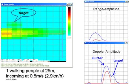
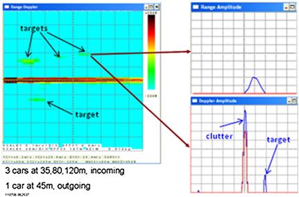
Other sensors
In this section we consider the Unattended Ground Passive Sensors (UGPS) and Electro-Optic (EO) to detect moving people or vehicles.
UGPS. They are used in case of small areas or critical infrastructure perimeter surveillance. They give alarms in presence of target in the operational range and, in some cases, can give a pre-classification of the target detected. The range of each sensor is usually limited to 10 m, but the latest technologies promise to reach detection ranges up to 50 m. They have very small dimension (less than 1 l volume) and low weight (less than 1 kg); they can be rapidly installed on rough ground or roads. Figure 22.25 gives an example of positioning of UGPS in an operative field. They are of following basic types:
• seismic: to detect seismic movement produced by vehicles wheels or people walking,
• acoustic: to detect vehicle engine noise,
• infrared: to detect differences in thermal data from the environment due to the infrared signature of people and vehicles,
• magnetic: to detect magnetic filed variation produced by vehicles.
Electro-Optic: They are widely used for surveillance, and many signal processing techniques assist the operator for target detection alerts.
They can be fixed or rotating covering up to 360° in azimuth. For the night vision infrared EO are used, either passive or active, and they can reach a visibility of several kilometers in range. The EO are normally used stand alone or connected with radar sensor to help the operator for classification and identification of the detected targets. For example, with active infrared the operator can read (up to 2 km far from the camera) the license plate of a vehicle previously detected and tracked by the radar.
2.22.8.2.2 Sensor network
The sensors operate in cluster, and they are connected via a low power RF link, operating at UHF or L/S bands. The data of the unmanned radars can be combined with the data of other UGPS sensors (infrared, acoustic, seismic), or connected to an existing network, to perform a more reliable detection system.
In Figure 22.26 an example of sensor network is reported. As shown, adjacent sensor nodes are connected together and the information are sent, to the master station, via the short range radio link; the master station performs data fusion and medium range connection with the other master stations, or the C2 center. In case of long range connection the master stations are connected via radio link repeaters or satellite connections.

Special care must be taken to avoid interactions among the sensors, where two or more sensors share the same visibility area. Mutual interferences can be avoided using different frequencies and/or different timing for the transmitted waveform and also orthogonally coded waveforms.
The data transfer among the nodes is performed using the radio link between adjacent nodes. In case of linear geometric distribution the data grow up linearly with the number of nodes in the subnet; as a consequence the number of nodes in the subnet is limited by the maximum data rate of the single connection link.
The linear electronic fence can be composed of two or more parallel sections to allow redundancy in case of failure or loss of visibility of one or more sensors.
An example of electronic fence is shown in Figure 22.27. In this case different environment conditions have been considered (riverside, forest, manmade buildings, and obstacles) and a network of FOPEN unattended ground radar sensors is used.
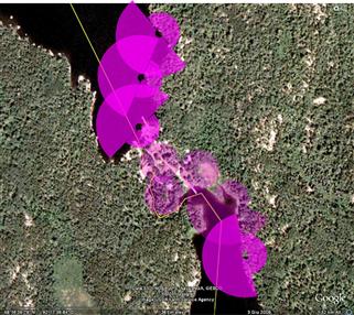
2.22.8.2.3 Fusion engine
The fusion engine allows to fuse heterogeneous sensor data at multiple levels to perform tracking and classification of relevant entities present in the scenario and to provide a high quality representation of the situation together with cartographic layers and sensed images of the terrain. Figure 22.28 provides an example of architecture for the fusion engine.
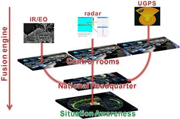
The tracking function processes the raw data provided by sensors and generates a set of tracks, representative of the real entities present in the scenario. A track typically carries the following information: a timestamp, position coordinates, velocity components, uncertainty on the kinematic components as expressed through the covariance matrix and additional attributes such as class/type and identity. In consideration of the potentially huge geographic extension of the system and of the importance to optimize the deployment of sensors as well as communication and processing power resources, a distributed tracking architecture is necessary. At the first level of the tracking architecture each sensor produces its own “local” tracks, in order to make available to the fusion engine a filtered information. Then a second level tracking combines local tracks originating from different sources into system tracks. This solution distributes the computational load on the peripheral nodes and reduces considerably the communication traffic which must be transmitted from the local level to the higher echelons; this is extremely important in consideration of the reduced bandwidth generally available between the peripheral elements and the center of the system.
In this step of the process, information of different nature can be fused producing a unique high quality information. Radar tracks can be fused with multiple images acquired by SAR and optical sensors, even if acquired at different resolutions, to achieve an improved representation of the scene with respect to the one achievable by processing data sets separately, in particular in terms of detection and false alarm probabilities when dealing with small targets (i.e., targets that occupy only few pixels of the image) [158–162]. The cartographic layers, superimposed with SAR or optical images, allow to put into context all the available information and support the fusion process (e.g., target tracking for ground vehicles especially during maneuvers).
Another output of the fusion engine is the classification of the tracked targets and entities of the scenario, i.e., the attribution of a class to the track under examination, hence supporting the capability to achieve a situation awareness.
From an operational point of view, the fusion engine can be considered as the responsible of producing a multi-resolution and multi-layer COP (Common Operating Picture), whose definition, as provided by [163], is the following: “A single identical display of relevant information shared by more than one command that facilitates collaborative planning and assists all echelons to achieve situational awareness.” The COP therefore provides to the operators at the different levels the capability to view each time a well-suited map, both in terms of proper scale (with respect to the scale of the observed situation) as well as in terms of number and type of information, according to the situation under analysis. This characteristic allows the system to properly support the operator without overloading him with unimportant information and keep him focused on events and information that might be related with his goal in terms of spatial, temporal, and logic correlation.
In the following the main constituents of the fusion engine are described.
Local tracking
The local tracking function processes the measurements provided by the sensor and produces a local track for each of the observed targets present in the surveillance region. The task of the tracking function at the local level is therefore of using the measurements made available by the sensor to estimate the number of targets and their kinematic components [164–166]. Local tracks provide position and velocity estimates at a given time, together with an indication of track quality; the track may also include other attributes relative to track classification, derived directly from radar measurements, from other sensors (EO/IR, UGPS, UAV) or assigned by a human operator.
In the scenario of a generic land border may be necessary to form low altitude tracks, surface tracks and ground tracks. Tracking of ground targets is especially critical due to the characteristics of the ground environment and of ground targets. The main criticality may be the masking effect due to terrain orography and vegetation. Another interesting feature of the ground environment is the presence of areas, mainly roads, where the probability of finding targets is higher, and areas such as off-road where the presence of targets is less probable. Distinguishing features of ground targets are high maneuverability and move-stop-move dynamics.
Even a well trained operator would be unable to select the correct hypothesis when a ground target is maneuvering since available information is insufficient. In these situations the best strategy is to defer the final decision until more data is available. To take into account these difficulties, the tracking function must be designed so as to handle several concurrent hypotheses and to make final decisions with a deferred logic [167–169], i.e., when more data is available which allows to make a final decision with sufficient confidence. The choice of hypotheses is also dependent on the environment and on the target type. The management of multiple hypotheses is then the capability of the function to consider at each time instant a set of hypotheses, such as:
• the target is proceeding regularly/is maneuvering on road;
The tracking function assigns a score to each hypothesis and identifies the most probable; the function keeps alive for some time not only the most likely hypothesis but also a set of alternative hypotheses which represent different kinematic evolutions of the target. Figure 22.29 shows an example of the set of hypotheses generated by the function: each hypothesis is relative to a path in the tree from time t0 to time t3 and the single branches may be relative to the choice of a specific dynamic model and/or a specific correlation hypothesis with a measurement in the set. For example in the path highlighted in red it is assumed that the target trajectory in the interval t0–t3 is described by the dynamic model m1; the other branches are relative to alternative hypotheses where it is assumed for example that the target has maneuvered (m2) or stopped (m3), etc. As new information is acquired, the probability of each hypothesis is updated according to new information; hypothesis which initially have a low score may gain credibility and vice versa. This characteristic, i.e., defer the decision until the available information is considered sufficient, allows to resolve most critical situations.
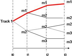
To take into account terrain and geographic information, the tracking solution leverages also context information provided by the GIS (Geographic Information System) in accordance with logics of terrain and road aided tracking. Digital Terrain Elevation Data (DTED) are also used to perform accurate projections of the tracks on the terrain and to identify zones where the target trajectory will be masked by obstacles and thus improve track continuity and the estimate of track kinematic parameters (e.g., maximum target velocity given the terrain type). The following Figure 22.30 shows, for instance, how environmental knowledge can be exploited to improve the tracking function [170,171]. Figure 22.30a shows a landscape covered by forests and crossed by a network of paths; due to the nature of the environment, targets especially if motorized, will preferentially move along the track, avoiding off-road areas more difficult to traverse. The blue line represents the trajectory of a track which moves along a winding path in the forest. Figure 22.30b on the other side shows how information relative to roads and viability in general can be exploited to improve the tracking performance. When the track approaches a bifurcation or a crossing, different hypotheses are generated to take into account possible target trajectories, such as on-road, off-road and also move-stop motion. More specifically the adoption of techniques such as road aided tracking is specifically important since it allows to improve the accuracy in the estimation of target kinematic parameters and therefore to make longer term projections. Finally weather information is exploited to further improve the tracking processing by feeding in information about areas where target detection is less probable (e.g., flooded areas) and expected target velocity is low given the past days weather conditions (e.g., heavy rain is expected to result in limited target velocity).
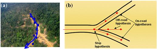
Classification
The classification function allows attributing a class to the track under examination, i.e., to determine its belonging to a class of targets. Target classification is extremely important since it helps to determine target identity and its threat level. Part of the classification process is the non-cooperative target recognition (NCTR), in order to avoid fratricide and to allow proper allocation of defensive means against the threat. In a coastal scenario NCTR capabilities are needed against ships, potentially involved in terrorism, illegal immigration or contraband operations, in order to assess and prioritize threats and to provide the appropriate response.
Sensors such as radar, EO/IR, may provide useful information for classification. In the radar case, the NCTR technology facilitates the identification of non-co-operative targets by transmitting wide band signals and by processing the radar echoes in a suitable multidimensional domain; e.g., time-frequency and range-angle. In the former case the target is discriminated on the basis of the jet engine or the helicopter rotor modulations of the echo [172–175]; in the latter case the target is discriminated on the basis of the measured two-dimensional radar image obtained by ISAR techniques [176–178] (Figure 22.31 shows a snapshot of the radar image of a ship).
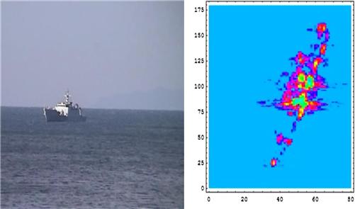
Figure 22.31 A snapshot of ISAR (Inverse SAR) signal processing, a profile of a ship along range and cross-range.
The automatic classification, that the radar is capable of providing by means of these processing techniques, is used directly within the tracking function, to support the plot-track correlation process and to attribute a class to the track. The classification process allows therefore determining the class to which the track belongs (such as pedestrians, vehicles, convoys, helicopters, and small low altitude aircrafts) and performing cueing to other sensors (e.g., EO/IR sensors, high resolution radars) or demanding a patrolling mission (e.g., a mission with UAV).
While data provided by sensors are needed to perform the classification processing, once the target has been assigned to a class, this information can be exploited at sensor level to achieve better accuracy in the performed processing (e.g., target classification can be used to refine kinematic target parameters used in the tracking processing).
The range-Doppler information can be furthermore employed to produce a confusion matrix useful for target classification. The confusion matrix expresses the a posteriori probability that a target has been classified correctly among a finite number of classes that have been a priori established. References [21,179] give an example of the use of confusion matrix in the classification issue.
2.22.9 Estimation and forecasting of an epidemic
Epidemics can impose serious challenges on societies in modern times. The poor health of general population due to a disease causes hardship and pain but also negative trends in the economy through absenteeism from work, missed business opportunities, etc. The ongoing epidemics of AIDS (Acquired Immune Deficiency Syndrome), tuberculosis and the recent outbreaks of SARS (Severe Acute Respiratory Syndrome) and H1N1 (swine flu) provide some revealing examples.
In the absence of an effective cure against an infectious disease, the best approach to mitigate its malicious or natural epidemic outbreak resides in the development of a capability for its early detection and prediction of its further development [180]. This enables typical countermeasures, such as the quarantine, vaccination, medical treatment, to be much more effective and less costly [181,182]. Therefore this issue can be approached as a surveillance problem in the context of Homeland Protection.
Syndromic surveillance is referred to as a systematic collection, analysis, and interpretation of public health data for the purpose of early detection of an epidemic outbreak and the mobilization of a rapid response [180,182]. The key idea is to detect an epidemic outbreak using early symptoms, well before the clinical or laboratory data result in a definite diagnosis. The rationale is that a spread of an infectious disease is usually associated with the measurable changes in the social behavior, which can be measured by non-medical means. Recent studies [183–185] have demonstrated that these non-medical sources of syndromic data streams, such as the absenteeism from work/school, the pharmaceutical sales, internet queries, twitter messages, and alike, can enable one to draw important conclusions regarding the epidemic state in the community. The “Google Flu” project [186] (flu-related searches in Google) is a well publicized example of this approach.
The algorithms for syndromic surveillance and have recently attracted significant attention by scientists and practitioners; there is a vast amount of literature devoted to this topic (for more comprehensive review see [180,182] and references therein). In general, all algorithms applied in this area can be divided into two main groups, the data mining methods and the information fusion (also known as data assimilation) methods. Data mining is primarily concerned with the extraction of patterns from massive amounts of raw data without using dynamic models of the underlying process (i.e., epidemic spread) [183,185]. Information fusion algorithms, on the contrary, strongly rely of mathematical models: in this case, the dynamic model of an epidemic outbreak and the measurement model of a particular syndromic data stream [187,188]. Naturally, the accuracy of information fusion algorithms is significantly determined by the fidelity of the underlying models.
This section presents a study of a recursive information fusion algorithm for syndromic surveillance, formulated in the Bayesian context of stochastic nonlinear filtering and solved using a particle filter [134]. While a similar work has been considered earlier, see [189–192], this section introduces two novelties. First, in order to overcome the limitations of the standard “compartment” model of epidemic spread (the “well-mixed” approximation) we employ a more flexible alternative, see [193,194]. The adopted epidemic model has the explicit parameter of “mixing efficiency” (or level of social interaction) and is therefore more appropriate to represent a variety of social interactions in a small community (e.g., self-isolation and panic). An advantage of the adopted epidemiological model is also that it enables to estimate the scaling law of the noise level with respect to the population size of a community. Second, a more flexible model of syndromic measurements, validated with data sets available in the literature [183,186], is adopted in the section. This measurement model is robust in the sense that some of its parameters are specified imprecisely, as interval values. The optimal sequential estimator (filter) and predictor are then formulated in the Bayesian framework and solved using a particle filter.
2.22.9.1 Modeling
To describe the dynamics of an epidemic outbreak we employ the generalized SIR (Susceptible, Infectious and Recovered) epidemic model with stochastic fluctuations [195–197]. According to this model, the population of a community can be divided into three interacting groups: susceptible, infectious and recovered. Let the number of susceptible, infectious and recovered be denoted by S, I, and R, respectively, so that S + I + R = P, where P is the total population size. The dynamic model of epidemic progression in time can be then expressed by two stochastic differential equations subject to the “conservation” law for the population:
 (22.46)
where ![]() , and
, and ![]() are two uncorrelated white Gaussian noise processes, both with zero mean and unit variance. The terms
are two uncorrelated white Gaussian noise processes, both with zero mean and unit variance. The terms ![]() and
and ![]() are introduced into Eq. (22.46) to capture the demographic noise (random variations in the contact rate
are introduced into Eq. (22.46) to capture the demographic noise (random variations in the contact rate ![]() and in the recovery time
and in the recovery time ![]() ) [197,198]. Parameter
) [197,198]. Parameter ![]() in Eq. (22.46) is the population mixing parameter, which for a homogeneous population equals 1. In the presence of an epidemic, however,
in Eq. (22.46) is the population mixing parameter, which for a homogeneous population equals 1. In the presence of an epidemic, however, ![]() may vary as people change their daily habits to reduce the risk of infection (e.g., panic, self-isolation). In general, model parameters
may vary as people change their daily habits to reduce the risk of infection (e.g., panic, self-isolation). In general, model parameters ![]() can be assumed to be partially known as interval values. In order to insure
can be assumed to be partially known as interval values. In order to insure ![]() , standard deviations
, standard deviations ![]() need to satisfy [199]:
need to satisfy [199]:
![]() (22.47)
(22.47)
Assuming that non-medical syndromic data are available for estimation and forecasting of the epidemic, we adopt a measurement model verified by [185,186], where a power law relationship holds for the odds-ratio between the observable syndrome ![]() and the (normalized) number of infected people i:
and the (normalized) number of infected people i:
![]() (22.48)
(22.48)
The power law exponent ![]() in Eq. (22.48) is in general syndrome specific. Since at the initial stages of an epidemic (which is of main interest for early detection and forecasting) we have:
in Eq. (22.48) is in general syndrome specific. Since at the initial stages of an epidemic (which is of main interest for early detection and forecasting) we have: ![]() and
and ![]() , Eq. (22.48) can be reduced to a simple power-law model:
, Eq. (22.48) can be reduced to a simple power-law model:
![]() (22.49)
(22.49)
where ![]() is a constant and
is a constant and ![]() is introduced to model the random nature of measurement noise. It is assumed that
is introduced to model the random nature of measurement noise. It is assumed that ![]() is uncorrelated to other syndromes and dynamic noises
is uncorrelated to other syndromes and dynamic noises ![]() . Since
. Since ![]() (e.g., number of Google searches), the noise term
(e.g., number of Google searches), the noise term ![]() associated with syndrome j should be modeled by a random variable that provides strictly non-negative realizations. For this purpose we adopt the log-normal distribution, that is
associated with syndrome j should be modeled by a random variable that provides strictly non-negative realizations. For this purpose we adopt the log-normal distribution, that is ![]() , with
, with ![]() and
and ![]() being the standard Gaussian distribution.
being the standard Gaussian distribution.
Parameters ![]() typically are not known, but with a representative data set of observations the model of Eq. (22.49) can be easily calibrated (see for example the results of the linear regression fits in [186]). The data fit reported in [183] suggests that
typically are not known, but with a representative data set of observations the model of Eq. (22.49) can be easily calibrated (see for example the results of the linear regression fits in [186]). The data fit reported in [183] suggests that ![]() may be close to unity, although it is difficult to precisely specify its value because of significant scattering of data points). To cater for this uncertainty, we assume that
may be close to unity, although it is difficult to precisely specify its value because of significant scattering of data points). To cater for this uncertainty, we assume that ![]() can take any value in an interval,
can take any value in an interval, ![]() around
around ![]() . Unfortunately [185,186] do not report any specific values of fitting parameters, so we use in this study some heuristic values for
. Unfortunately [185,186] do not report any specific values of fitting parameters, so we use in this study some heuristic values for ![]() in our simulations.
in our simulations.
The problem now is to estimate the (normalized) number of infected i, and susceptible s at time t, using syndromic observations ![]() of Eq. (22.49), collected up to time t. Let x denote the state vector to be estimated; it includes i and s, but also the imprecisely known epidemic model parameters
of Eq. (22.49), collected up to time t. Let x denote the state vector to be estimated; it includes i and s, but also the imprecisely known epidemic model parameters ![]() and
and ![]() . The formal Bayesian solution is given in the form of the posterior pdf
. The formal Bayesian solution is given in the form of the posterior pdf ![]() , where
, where ![]() is the state vector at time t and
is the state vector at time t and ![]() denotes all observations up to time t. Using the posterior
denotes all observations up to time t. Using the posterior ![]() , one can predict the progress of the epidemic using the dynamic model of Eq. (22.46).
, one can predict the progress of the epidemic using the dynamic model of Eq. (22.46).
2.22.9.2 Sequential Bayesian solution
For the purpose of computer implementation, first we need a discrete-time approximation of dynamic model of Eq. (22.46). The state vector is adopted as: ![]() , where T is the matrix transpose. Using Euler’s method with small integration interval
, where T is the matrix transpose. Using Euler’s method with small integration interval ![]() , the nonlinear differential equations in Eq. (22.46) can be approximated as
, the nonlinear differential equations in Eq. (22.46) can be approximated as
![]() (22.50)
(22.50)
where ![]() is the discrete-time index and
is the discrete-time index and
 (22.51)
is the transition function; here ![]() denotes the ith component of vector
denotes the ith component of vector ![]() . Discrete-time process noise
. Discrete-time process noise ![]() in Eq. (22.50) is assumed to be zero-mean white Gaussian with diagonal covariance matrix
in Eq. (22.50) is assumed to be zero-mean white Gaussian with diagonal covariance matrix ![]() , which according to Eq. (22.47) can be expressed as
, which according to Eq. (22.47) can be expressed as ![]() .
.
The optimal Bayes filter is typically presented in two steps, prediction and update. Suppose the posterior pdf at time ![]() is given by
is given by ![]() . Then the prediction step computes the pdf predicted to time
. Then the prediction step computes the pdf predicted to time ![]() as [194]:
as [194]:
![]() (22.52)
(22.52)
where ![]() is the transitional density. According to Eq. (22.50), we can write
is the transitional density. According to Eq. (22.50), we can write ![]() . The prediction step is carried out many times with tiny sampling intervals
. The prediction step is carried out many times with tiny sampling intervals ![]() until observation
until observation ![]() about syndrome j becomes available at
about syndrome j becomes available at ![]() . The predicted pdf at
. The predicted pdf at ![]() is denoted
is denoted ![]() .
.
In the standard Bayesian estimation framework, the predicted pdf is updated using measurement ![]() by multiplication with the measurement likelihood function [200]. According to Eq. (22.49), the likelihood function in this case is
by multiplication with the measurement likelihood function [200]. According to Eq. (22.49), the likelihood function in this case is ![]() , where
, where ![]() . The standard Bayesian approach, however, cannot be applied because
. The standard Bayesian approach, however, cannot be applied because ![]() defined in this way is not a function:
defined in this way is not a function: ![]() is effectively an infinite set (an interval) and therefore
is effectively an infinite set (an interval) and therefore ![]() is one-to-many mapping.
is one-to-many mapping.
An elegant solution to the imprecise measurement transformation is available in the framework of random set theory [137]. In this approach ![]() is modeled by a random set
is modeled by a random set ![]() and the likelihood function represents the probability:
and the likelihood function represents the probability:![]() , and is referred to as the generalized likelihood. More details and a theoretical justification of this approach can be found in [201]. The Bayes update using syndromic measurement
, and is referred to as the generalized likelihood. More details and a theoretical justification of this approach can be found in [201]. The Bayes update using syndromic measurement ![]() is now defined as [137]:
is now defined as [137]:
![]() (22.53)
(22.53)
For the measurement model Eq. (22.49) with additive Gaussian noise, the generalized likelihood has an analytic expression [201]:
![]() (22.54)
(22.54)
where ![]() define the limits of the set and
define the limits of the set and ![]() is the cumulative log-normal distribution. The recursions of the Bayes filter start with an initial pdf (at time
is the cumulative log-normal distribution. The recursions of the Bayes filter start with an initial pdf (at time ![]() , denoted
, denoted ![]() , which is assumed known.
, which is assumed known.
The proposed Bayesian estimator cannot be solved in the closed form. Instead we developed an approximate solution based on the particle filter (PF) [134,202]. The PF approximates the posterior pdf ![]() by a weighted random samples; details can be found in [134,202]. The only difference here is that importance weight computation is based on the generalized likelihood function.
by a weighted random samples; details can be found in [134,202]. The only difference here is that importance weight computation is based on the generalized likelihood function.
2.22.9.3 Numerical results
Epidemic forecasting will be demonstrated using an experimental data set obtained using a large-scale agent based simulation model [203,204] of a virtual town of P = 5000 inhabitants, created in accordance with the Australian Census Bureau data. The agent based model is rather complex (takes a long time to run) and incorporates a typical age/gender breakdown, family-household-workplace habits, including the realistic day-to-day people contacts for a disease spread. The blue line in Figure 22.32 shows the number of people of this town infected by a fictitious disease, reported once per day during a period of 154 days (only first 120 days shown). The dashed red line represents the adopted SIR model fit, using the entire batch of 154 data points and integration interval ![]() days, with no process noise, i.e.,
days, with no process noise, i.e., ![]() in Eq. (22.50). The estimated model parameters are:
in Eq. (22.50). The estimated model parameters are: ![]() . These estimates were obtained using the importance sampling technique of progressive correction [202]. Figure 22.32 serves to verify that the adopted non-homogeneous mixing SIR model, although very simple and fast to run, is remarkably accurate in explaining the data obtained from a very complex simulation system.
. These estimates were obtained using the importance sampling technique of progressive correction [202]. Figure 22.32 serves to verify that the adopted non-homogeneous mixing SIR model, although very simple and fast to run, is remarkably accurate in explaining the data obtained from a very complex simulation system.
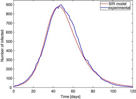
Figure 22.32 Experimental data set: the solid blue line represents the number of infected people over time (obtained by agent based simulation); the dashed red line is the fitted non-homogeneous mixing SIR model. (For interpretation of the references to color in this figure legend, the reader is referred to the web version of this book.)
The true number of infected people in forecasting simulations is chosen to be the output of the agent based population model, shown by the solid blue line in Figure 22.32. The measurements are generated synthetically in accordance with Eq. (22.49) and discussions above, using the following parameters: ![]() monitored syndromes. Independent measurements concerning all Nz = 4 syndromes are assumed available on a daily basis during the first 25 days. The problem is to perform the estimation sequentially as the measurements become available until the day number 25, and at that point of time to forecast the number of infected people as a function of time.
monitored syndromes. Independent measurements concerning all Nz = 4 syndromes are assumed available on a daily basis during the first 25 days. The problem is to perform the estimation sequentially as the measurements become available until the day number 25, and at that point of time to forecast the number of infected people as a function of time.
The initial pdf for the state vector was chosen as ![]() with
with ![]() , where
, where ![]() and
and ![]() denote the truncated Gaussian distribution, restricted to
denote the truncated Gaussian distribution, restricted to ![]() , and uniform distribution, respectively. The imprecise measurement parameter is adopted as
, and uniform distribution, respectively. The imprecise measurement parameter is adopted as ![]() , while its true value The number of particles is set to 10,000.
, while its true value The number of particles is set to 10,000.
Figure 22.33 shows the histograms of particle filter estimated values of ![]() , and
, and ![]() , after processing 25 days of syndromic data (i.e., in total 100 measurements). The histograms in this figure reveals that the uncertainty in parameters
, after processing 25 days of syndromic data (i.e., in total 100 measurements). The histograms in this figure reveals that the uncertainty in parameters ![]() and
and ![]() has been substantially reduced after processing the data (compared with the initial
has been substantially reduced after processing the data (compared with the initial ![]() and
and ![]() ). The uncertainty in
). The uncertainty in ![]() , on the other hand, has not been reduced, indicating that this parameter cannot be estimated from syndromic data. While this is unfortunate, it does not appear to be a serious problem in forecasting the epidemic mainly because the prior on
, on the other hand, has not been reduced, indicating that this parameter cannot be estimated from syndromic data. While this is unfortunate, it does not appear to be a serious problem in forecasting the epidemic mainly because the prior on ![]() in practice is fairly tight (
in practice is fairly tight ( ![]() ). This is confirmed in Figure 22.34 which shows a sample of 100 overlaid predicted epidemic curves (gray lines) based on the estimate of
). This is confirmed in Figure 22.34 which shows a sample of 100 overlaid predicted epidemic curves (gray lines) based on the estimate of ![]() obtained after 25 days. Figure 22.34 indicates that the forecast of the peak of the epidemic is fairly accurate, while the forecast of the size of the peak is more uncertain. Most importantly, however, the true epidemic curve (solid red line) appears to be always enveloped by the prediction curves. More experimental results can be found in [199].
obtained after 25 days. Figure 22.34 indicates that the forecast of the peak of the epidemic is fairly accurate, while the forecast of the size of the peak is more uncertain. Most importantly, however, the true epidemic curve (solid red line) appears to be always enveloped by the prediction curves. More experimental results can be found in [199].
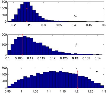
Figure 22.33 Histograms of particle filter estimated values of epidemic model parameters after processing 25 days of syndromic measurements. Red vertical lines indicate the true values. (For interpretation of the references to color in this figure legend, the reader is referred to the web version of this book.)
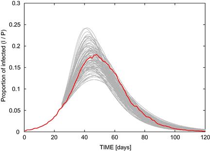
Figure 22.34 Prediction results for a random sample of 100 particles (gray lines); the red line is the experimental curve from Figure 22.32. (For interpretation of the references to color in this figure legend, the reader is referred to the web version of this book.)
2.22.10 Conclusions
Integrated sensor systems and data fusion have been the main focus of this chapter. The discussed matter has been subdivided in nine sections which have covered a long trip starting from the description of the Homeland Protection problem, to the illustration of a wide spectrum of information sources (sensors and the like), to the netting of such sensors (both homogeneous and heterogeneous), with a broad range of practical applications: cooperative sensing to defend a urban territory, network of cooperative chemical sensors, detection and localization of radioactive point sources, use of so-called electronic fence to protect long borderlines of a territory, up to the estimation and forecasting of an epidemic. This work, an unofficial collaboration between experts from industry, research centers and academia, has brought together a wide spectrum of competences scientific, technical/technological/systemic and on the field.
List of Acronyms
AIDS Acquired Immune Deficiency Syndrome
C4I Command, Control, Communications, Computers, and Intelligence
CBINT Chemical and Biological Intelligence
cdf Cumulative distribution function
COMINT Communications Intelligence
CSIP Collaborative Signal and Information Processing
CTR Cooperative Target Recognition
DIKW Data Information Knowledge and Wisdom)
DSC Dynamic Sensor Collaboration
DSTO Defense Science and Technology Organisation
DTED Digital Terrain Elevation Data
ECM Electronic Counter Measures
ESM Electronic Support Measurement
ESM Electronic Support Measures
FMCW Frequency Modulated Continuous Wave
GEMS Generic Error modeling System
GEOINT Geospatial Intelligence
GIS Geographic Information System
GMTI Ground Moving Target Indicator
IFF Identification Friend or Foe
JDL Joint Directors of Laboratories
LPI Low Probability of Intercept
MASINT Measurement and Signature Intelligence
MDL Minimum Description Length
NCTR Non-Cooperative Target Recognition
ODNA Office of Directors of National Intelligence
OODA Observe-Orient-Decide-Act)
OSINT Open-Source Intelligence
PCRLB Posterior cramer rao lower bound
pdf Probability density function
SARS Severe Acute Respiratory Syndrome
SIR Susceptible Infectious Recovered
References
1. Naisbitt J. Megatrends. GCP 1982.
2. Antony RT. Principles of Data Fusion Automation. Artech House 1995.
3. Doucet A, de Freitas N, Gordon N, eds. Sequential Monte Carlo Methods in Practice. New York: Springer Verlag; 2001.
4. Kalman RE. A new approach to linear filtering and prediction problems. Trans ASME – J Basic Eng. 1960;82:35–45.
5. Mutambara AGO. Decentralized Estimation and Control for Multi-Sensor Systems. CRC Press 1998.
6. Klir GJ, Bo Y. Fuzzy Logic: Theory and Applications. Prentice Hall PTR 1995.
7. Dempster AP. A generalization of Bayesian inference. J Roy Stat Soc. 1968;30:205–247.
8. Shafer G. A Mathematical Theory of Evidence. Princeton University Press 1976.
9. Smarandache F, Dezert J, eds. Advances and Applications of DSmT for Information Fusion. vol. 1. American Research Press 2004.
10. Smarandache F, Dezert J, eds. Advances and Applications of DSmT for Information Fusion. vol. 2. American Research Press 2004.
11. Farina A, Pardini S. Introduction to multiradar tracking system. Rivista Tecnica Selenia. 1982;8(1):14–26.
12. Farina A, Studer FA. Radar data processing. In: England: Researches Studies Press, John Wiley; 1985;Bowron P, ed. Introduction and Tracking. vol. I (Translated in Russian—Radio I Sviaz-, Moscow, 1993—and in Chinese—China Defense Publishing House in 1988).
13. Farina A, Studer FA. Data Processing. In: England: Researches Studies Press, John Wiley; 1986;Bowron P, ed. Advanced Topics and Applications. vol. 2 (Translated in Chinese—China Defence Publishing House in 1992).
14. Farina A. Target tracking with bearings-only measurements. Signal Process. 1999;78(1):81–88.
15. Farina A, Miglioli R. Association between active and passive tracks for airborne sensors. Signal Process. 1998;69(3):209–217.
16. Farina A, La Scala B. Methods for association of active and passive tracks for airborne sensors. In: Int Symp Radar, IRS98, Munich, Germany, September 15–17. 1998;735–744.
17. La Scala B, Farina A. Choosing a track association method. Inform Fusion J. 2002;3(2):119–133.
18. Waltz E, Llinas J. Multisensor Data Fusion. Norwood, MA: Artech House; 1990.
19. Hall D. Mathematical Techniques in Multisensory Data Fusion. Norwood, MA: Artech House; 1992.
20. Alberts DS, Garstka J, Stein FP. Network Centric Warfare: Developing and Leveraging Information Superiority. USA: National Defence Press; 1999.
21. Farina A, Graziano A, Ortenzi L, Spinogatti E. The role of modelling and simulation (M and S) in the analysis of integrated systems for homeland protection. In: Franceschetti G, Grossi M, eds. Homeland Security Technology Challenges, From Sensing and Encrypting to Mining and Modelling. Artech House 2008; (Chapter 9).
22. Skinner CJ, Cochrane S, Field M, Johnston R. Defence Against Terrorism: The Evolution of military Surveillance Systems into Effective Counter Terrorism Systems Suitable for Use in Combined Military Civil Environments, Dream or Reality? NATO Panel Systems, Concepts and Integration (SCI) Methods and Technologies for Defence Against Terrorism, London, UK,. October 2004; 25–27.
23. US Office of Homeland Security: National Strategy for Homeland Security, Washington, DC, July 2002. <http://www.whitehouse.gov/homeland/book/natstrathls.pdf>.
24. U.S. Environmental Protection Agency: Strategic Plan for Homeland Security, Washington, DC, September 2002. <http://www.epa.gov/epahome/downloads/epahomelandsecuritystrategicplan.pdf>.
25. J. Moteff, C. Copeland, J, Fischer, Critical Infrastructure: What Makes an Infrastructure Critical? Report for Congress RL31556, The Library of Congress, August 2002. <www.fas.org/irp/crs/RL31556.pdf>.
26. US Government, The National Strategy for the Physical Protection of Critical Infrastructure and Key Assets, The White House, Washington, DC, February 2003.
27. S. Bologna, R. Setola, The need to improve local self-awareness in CIP/CIIP, in: Proceeding of 1st IEEE Int. Workshop on CIP (IWCIP 2005), Darmstadt, Germany, November 3–4, 2005, pp. 84–89.
28. Rinaldi S, Peerenboom J, Kelly T. Identifying, understanding and analyzing critical infrastructure interdependencies. IEEE Control Syst Mag. 2001;21(6):11–25.
29. <http://www.icc-ccs.org/piracy-reporting-centre>.
30. Archive of International Maritime Bureau Piracy and Armed Robbery Reports, IMB Publications, 2008.
31. Farina A, Giompapa S, Graziano A. Decision making and the vulnerability of interdependent critical infrastructure. In: Franceschetti G, Grossi M, eds. Homeland Security–Facets: Threats, Countermeasures, and the Privacy Issue. Artech House 2011; (Chapter 4).
32. Zimmerman R. Making and the vulnerability of interdependent critical infrastructure. In: Proceeding of the IEEE Conference on Systems, Man and Cybernetics 2004. The Netherlands: The Hague; October 2004;4059–4063. 10–13.
33. R. Setola, S. Geretshuber, Critical information infrastructure security, in: Third International Workshop CRITIS, Frascati (Rome), Italy, October 2008, pp. 13–15.
34. Smith ST, Silberfarb A, Philips S, Kao EK, Anderson C. Network discovery using wide-area surveillance data. In: Proceedings of IEEE Conference on Information Fusion 2011, Lexington, MA, USA. July 2011;1–8. 5–8.
35. Starr A, Desforges M. Strategies in data fusion–sorting through the tool box. In: Bedworth, O’Brien, eds. Proceedings of EuroFusion98 International Conference on Data Fusion. 1998;85–90.
36. Steinberg AN, Bowman CL. A systems engineering approach for implementing data fusion systems. In: Hall DL, Llinas J, eds. Handbook of Multisensor Data Fusion. London: CRC Press; 2001.
37. White FE. A model for data fusion. In: 1988;143–158. Proceedings of the 1st National Symposium on Sensor Fusion, Chicago, USA. vol. 2.
38. Steinberg AN, Bowman CL, White FE. Revisions to the JDL data fusions models. In: Proceedings of the 3rd NATO/IRIS Conference, Quebec City, Canada. 1998.
39. Blasch E, Plano S. JDL Level 5 fusion model: user refinement issues and applications in group tracking. In: 2002;270–279. Proceedings of the SPIE Signal Processing Sensor Fusion Target Recognition XI. vol. 4729.
40. Blasch E, Plano S. Level 5: user refinement to aid the fusion process. Proceedings of the SPIE Multisensor, Multisource Information Fusion: Architectures, Algorithms, and Applications. 2003;vol. 5099:288–297.
41. Blasch E, Plano S. DFIG Level 5: user refinement issues supporting situational assessment reasoning. In: Proceedings of 8th International Conference on Information Fusion, Philadelphia, USA. July 2005;25–29.
42. Subrata Das. High-Level Data Fusion. Artech House 2008.
43. Rowley J. The wisdom hierarchy: representations of the DIKW hierarchy. J Inform Sci. 2007;33(2):163–180.
44. Endsley MR. Design and evaluation for situation awareness enhancement. In: Proceedings of the 32nd Annual Meeting of the Human Factors Society. 1988;97–101.
45. Endsley MR. Toward a theory of situation awareness in dynamic systems. Human Factors. 1995;37(1):32–64.
46. Endsley MR. Measurement of situation awareness in dynamic systems. Human Factors. 1995;37(1):65–84.
47. Perla PP, Markowitz M, Nofi AA, Weuve C, Loughran J, Stahl M. Gaming and shared situation awareness, Alexandria, Virginia, Centre for Naval Analyses. 2000.
48. J.R. Boyd, A Discourse on Winning and Losing, Unpublished Set of Briefing Slides, Air University Library, Maxwell AFB, AL, USA, May, 1987.
49. Bass T. Intrusion detection systems and multisensor data fusion: creating cyberspace situational awareness. Commun ACM. 2000;43(4):99–105.
50. Bedworth MD, O’Brien J. The omnibus model: a new architecture for data fusion? IEEE Trans Aerosp Electron Syst. 1999;15(4):30–36.
51. Rasmussen J. Skills, rules and knowledge: signals, signs and symbolism, and other distinctions in human performance models. IEEE Trans Syst Man Cybern. 1983;12:257–266.
52. Rasmussen J. Information Processing and Human Machine Interaction: An Approach to Cognitive Engineering. NY: North Holland; 1986.
53. Reason J. Human Error. Cambridge, UK: Cambridge University Press; 1990.
54. USAF (United States Air Force): Air Force Pamphlet 14–210, Intelligence, USAF Intelligence Targeting Guide, Department of Defense, USA, 1998.
55. ODNI (Office of Director of National Intelligence): How Do We Collect Intelligence? USA, 2008. <http://www.dni.gov/whowhat/whatcollection.htm>.
56. Krioukov D, Papadopoulos F, Vahdat F, Boguna M. Curvature and temperature of complex networks. Phys Rev E. 2009;80:035101(R).
57. Durrant-Whyte HF. Sensor models and multi-sensor integration. Int J Robot Res. 1988;7(6):97–113.
58. W. Elmenreich, Sensor fusion in time-triggered systems, PhD Thesis, Institut für Technische Informatik, Vienna University of Technology, 2002.
59. Kay SM. Statistical Signal Processing: Detection Theory. Prentice Hall 1998.
60. Farina A, Ristic B, Timmoneri L. Cramer-Rao bound for nonlinear filtering with Pd 1 and its application to target tracking. IEEE Trans Signal Process. 2002;50(8):1916–1924.
61. Hernandez M, Ristic B, Farina A, Timmoneri L. A comparison of two Cramer-Rao bounds for non-linear filtering with Pd < 1. IEEE Trans Signal Process. 2004;52(9):2361–2370.
62. Farina A, Ristic B, Immediata S, Timmoneri L. CRLB with Pd 1 fused tracks, Fusion 2005. In: Proceedings of the 7th International Conference on Information Fusion, Philadelphia, USA. July 2005;191–196. 25–28.
63. Nohara TJ, Weber P, Jones G, Ukrainec A, Premji A. Affordable high-performance radar networks for homeland security applications, RADAR ’08. In: Proceedings of IEEE International Radar Conference, Rome, Italy. May 2008;1–6. 26–30.
64. Nohara TJ, Weber P, Premji A, et al. Affordable avian radar surveillance systems for natural resource management and BASH applications, RADAR 2005. In: Proceedings of IEEE International Radar Conference, Arlington, Virginia, USA. May 2005;10–15. 9–12.
65. Proceedings of 2nd Workshop on Cognitive Information Processing, Elba Island, Tuscany, Italy, June 14–16, 2010.
66. Masazade R, Niu PK, Varshney M Keskinoz. Energy aware iterative source localization for wireless sensor networks. IEEE Trans Signal Process. 2010;58(9):4824–4835.
67. Zhao Feng, Shin Jaewon, Reich J. Information-driven dynamic sensor collaboration. IEEE Signal Process Mag. 2002;19(2):61–72.
68. Kreucher CM, Hero AO, Kastella KD, Morelande MR. An information-based approach to sensor management in large dynamic networks. Proc IEEE. 2007;95(5):978–999.
69. Williams JL, Fisher JW, Willsky AS. Approximate dynamic programming for communication-constrained sensor network management. IEEE Trans Signal Process. 2007;55(8):4300–4311.
70. Zuo L, Niu R, Varshney PK. Conditional posterior Cramér–Rao lower bounds for nonlinear sequential Bayesian estimation. IEEE Trans Signal Process. 2001;59(1):1–14.
71. Zuo L, Niu R, Varshney PK. Posterior CRLB based sensor selection for target tracking in sensor networks, ICASSP 2007. In: Hawaii: Honolulu; April 2007;II-1041–II-1044. IEEE International Conference on Acoustic Speech and Signal Processing. vol. 2 15–20.
72. Zuo L, Niu R, Varshney PK. A sensor selection approach for target tracking in sensor networks with quantized measurements. In: IEEE International Conference on Acoustic Speech and Signal Processing, ICASSP 2008, Las Vegas, Nevada, USA. 2008;2521–2524. March 30–April 4.
73. Hernandez ML, Kirubarajan T, Bar-Shalom Y. Multi-sensor resource deployment using posterior Cramer-Rao bounds. IEEE Trans Aerosp Electron Syst. 2004;40(2):399–416.
74. Collier TC, Taylor C. Self-organization in sensor networks. J Parall Distr Comput. 2004;64(7):866–873.
75. Cattivelli FS, Sayed AH. Modelling bird flight formations using diffusion adaptation. IEEE Trans Signal Process. 2011;59(5):2038–2051.
76. Cattivelli FS, Sayed AH. Distributed detection over adaptive networks using diffusion adaptation. IEEE Trans Signal Process. 2011;59(5):1917–1932.
77. Lopes CG, Sayed AH. Diffusion least-mean squares over adaptive networks: formulation and performance analysis. IEEE Trans Signal Process. 2008;56(7):3122–3136.
78. Cattivelli FS, Sayed AH. Diffusion LMS strategies for distributed estimation. IEEE Trans Signal Process. 2010;58(3):1035–1048.
79. Cattivelli FS, Lopes CG, Sayed AH. Diffusion recursive least-squares for distributed estimation over adaptive networks. IEEE Trans Signal Process. 2008;56(5):1865–1877.
80. Pikovsky A, Rosenblum M, Kurths J. Synchronization – A Universal Concept in Non Linear Sciences. Cambridge, UK: Cambridge University Press; 2001.
81. Lynch NA. Distributed Algorithms. San Mateo, CA: Morgan-Kaufmann; 1997.
82. Olfati-Saber R, Shamma JS. Consensus filters for sensor networks and distributed sensor fusion. In: Proceeding of the Joint IEEE Conference On Decision and Control and the European Control Conf., Seville, Spain. 2005;6698–6703. December 15.
83. Hong YW, Cheow LF, Scaglione A. A simple method to reach detection consensus in massively distributed sensor networks. In: Proceedings of International Symposium on Information Technology, ISIT 2004, Chicago, USA. July 2004;250.
84. Lucarelli D, Wang IJ. Decentralized synchronic protocols with nearest neighbor communication. In: Proceedings of the 2nd International Conference on Embedded Networked Sensor System, SenSys 2004, Baltimore, USA. November 2004;62–68. 3–5.
85. Barbarossa S. Self-organizing sensor networks with information propagation based on mutual coupling of dynamic systems. In: Proceedings of International Workshop on Ad-hoc Wireless Network 2005, IWWAN 2005, London, UK. May 2005; 23–26.
86. Barbarossa S, Scutari G. Decentralized maximum likelihood estimation for sensor networks composed of nonlinearly coupled dynamical systems. IEEE Trans Signal Process. 2007;55(7-I):3456–3470.
87. Scutari G, Barbarossa S, Pescosolido L. Distributed decision through self-synchronizing sensor networks in presence of propagation delays and asymmetric channels. IEEE Trans Signal Process. 2008;56(4):1667–1684.
88. Barbarossa S, Scutari G, Swami A. Achieving consensus in self-organizing wireless sensor networks, the impact of network topology on energy consumption. In: Hawaii: Honolulu; April 15–20, 2007;841–844. Proceedings of ICASSP 2007. vol. 2.
89. Barbarossa S, Scutari G. Bio-inspired sensor network design. IEEE Signal Process Mag. 2007;24(3):26–35.
90. Fortunati S, Gini F, Greco MS, Farina A, Graziano A, Giompapa S. Least squares estimation and Cramér-Rao type lower bounds for relative sensor registration process. IEEE Trans Signal Process. 2011;59(3):1075–1087.
91. Zhou Yifeng, Leung H, Yip PC. An exact maximum likelihood registration algorithm for data fusion. IEEE Trans Signal Process. 1997;45(6):1560–1573.
92. Li Zhenhua, Chen Siyue, Leung H, Bosse E. Joint data association, registration, and fusion using EM-KF. IEEE Trans Aerosp Electron Syst. 2010;46(2):496–507.
93. Chen Siyue, Leung H, Bosse E. A maximum likelihood approach to joint registration, association and fusion for multi-sensor multi-target tracking. In: Proceedings of 12th International Conference on Information Fusion, FUSION 2009, Seattle, USA. July 2009;686–693. 6–9.
94. Herzel S, Recchioni MC, Zirilli F. A quadratically convergent method for linear programming. Linear Algebra Appl. 1991;152:255–289.
95. Karmarkar N. A new polynomial time algorithm in linear programming. Combinatorica. 1984;4:373–395.
96. Hageman L, Young D. Applied Iterative Methods. New York: Academic Press; 1981.
97. Farina A, Graziano A, Mariani F, Zirilli F. A cooperative sensor network: optimal deployment and functioning. RAIRO Oper Res. 2009;44(4):379–388 (special issue COGIS).
98. Aurenhammer F. Voronoi diagrams–a survey of a fundamental geometric data structure. ACM Comput Surv. 1991;23(3):345–405.
99. Snyman JA. Practical Mathematical Optimization: An Introduction to Basic Optimization Theory and Classical and New Gradient-Based Algorithms. Cambridge, Massachusetts, USA: Springer; 2005.
100. Chung FR. Spectral Graph Theory. Providence, USA, CBMS 92: American Mathematical Society; 1997.
101. DeGroot MH, Schervish MJ. Probability and Statistics. New York: Pearson Addison Wesley; 2002.
102. Raghavendra CS, Sivalingam KM, Taieb Znati. Wireless Sensor Networks. USA: Springer; 2005.
103. Ertin E, Fisher JW, Potter LC. Maximum mutual information principle for dynamic sensor query problems. Lect Notes Comput Sci Inform Process Sensor Networks. 2003;2634:91–104.
104. Zhao F, Shin J, Reich J. Information-driven dynamic sensor collaboration for tracking applications. IEEE Signal Process Mag. 2002;19(2):61–72.
105. J. Mathieu, G. Hwang, J. Dunyak, The State of the Art and the State of the Practice: Transferring Insights from Complex Biological Systems to the Exploitation of Netted Sensors in Command and Control Enterprises, MITRE Technical Papers, MITRE Corporation, USA, July 2006.
106. Khelil A, Becker C, Tian J, Rothermel K. An epidemic model for information diffusion in MANETs. In: Proceedings of the 5th ACM International Workshop on Modeling Analysis and Simulation of Wireless and Mobile Systems, MSWiM 2002, Atlanta, Georgia, USA. Springer September 2002;54–60. 28.
107. De P, Liu Y, Das SK. An epidemic theoretic framework for evaluating broadcast protocols in wireless sensor networks. In: Proceedings of the 4th IEEE International Conference on Mobile Ad-hoc and Sensor Systems, MASS 2007, Pisa, Italy. October 2007;1–9. 8–11.
108. Ristic B, Skvortsov A, Morelande M. Predicting the progress and the peak of an epidemics. In: Proceedings of IEEE International Conference on Acoustics, Speech and Signal Processing 2009, ICASSP 2009, Taiwan. April 2009;513–516. 19–24.
109. Dekker A, Skvortsov A. Topological issues in sensor networks. In: MODSIM 2009: 2009 MSSANZ International Congress on Modelling and Simulation, Cairns, Australia. July 2009;952–958. 13–17.
110. Eubank S, Anil Kumar VS, Marathe M. Epidemiology and wireless communication: tight analogy or loose metaphor? Lect Notes Comput Sci Bio-Inspir Comput Commun. 2008;5151:91–104.
111. Bisignanesi V, Borgas MS. Models for integrated pest management with chemicals in atmospheric surface layers. Ecol Modell. 2007;201(1):2–10.
112. Skvortsov A, Ristic B, Morelande M. Networks of chemical sensors: a simple mathematical model for optimisation study. In: 5th International Conference on Intelligent Sensors, Sensor Networks and Information Processing, ISSNIP 2009, Melbourne, Australia. December 2009;385–390. 7–10.
113. Gunatilaka A, Ristic B, Skvortsov A, Morelande M. Parameter estimation of a continuous chemical plume source. In: IEEE 11th International Conference on Information Fusion, FUSION 2008, Cologne, Germany. 2008;1–8. June 30–July 3.
114. Murray JD. Mathematical Biology. vols. 8–12 Springer 2002.
115. Verhulst PF. Recherches mathématiques sur la loi d’accroissement de la population. Nouv mém de l’Academie Royale des Sci et Belles-Lettres de Bruxelles. 1845;18:1–41.
116. Weisstein EW, Logistic Equation, MathWorld-A Wolfram Web Resource. <http://mathworld.wolfram.com/LogisticEquation.html>.
117. Mendis C, Gunatilaka A, Skvortsov A, Karunasekera S. The effect of correlation of chemical tracers on chemical sensor network performance. In: Proceedings of 6th International Conference on Intelligent Sensors, Sensor Networks and Information Processing, ISSNIP 2010, Brisbane, Australia. December 2010;103–108. 7–10.
118. Skvortsov A, Ristic B. Modelling and performance analysis of a network of chemical sensors with dynamic collaboration. Int J Distr Sensor Networks 2012 2012; (article ID65231).
119. Karunasekera S, Mendis C, Skvortsov A, Gunatilaka A. A decentralized dynamic sensor activation protocol for chemical sensor networks. In: Proceedings of the 9th IEEE Symposium on Network Computing and Applications, Cambridge, MA, USA. July 2010;218–223. 15–17.
120. Karunasekera S, Beaton J, Dimech A, Skvortsov A, Gunatilaka A. A distributed e-research tool for evaluating source backtracking algorithms. In: Proceedings of IEEE 6th International Conference on e-Science, Brisbane, Australia. December 2010;17–24. 7–10.
121. Nemzek RJ, Dreicer JS, Torney DC, Warnock TT. Distributed sensor networks for detection of mobile radioactive sources. IEEE Trans Nucl Sci. 2004;51(4):1693–1700.
122. Brennan SM, Mielke AM, Torney DC. Radioactive source detection by sensor networks. IEEE Trans Nucl Sci. 2005;52(3):813–819.
123. Klimenko AV, Priedhorsky WC, Hengartner NW, Borozin KN. Efficient strategies for low-level nuclear searches. IEEE Trans Nucl Sci. 2006;53(3):1435–1442.
124. Sundaresan A, Varshney PK, Rao NSV. Distributed detection of a nuclear radioactive source using fusion of correlated decisions. In: Proceedings of IEEE International Conference on Information Fusion, FUSION 2007, Quebec, Canada. July 2007;1–8. 9–12.
125. Morelande MR, Ristic B. Radiological source detection and localisation using Bayesian techniques. IEEE Trans Signal Process. 2009;57(11):4220–4231.
126. Tsoulfanidis N. Measurement and Detection of Radiation. Washington, DC: Taylor and Francis; 1995.
127. Cortez RA, Papageorgiou X, Tanner HG, et al. Smart radiation sensor management. IEEE Robot Autom Mag. 2008;15(3):85–93.
128. Ristic B, Morelande MR, Gunatilaka A. Information driven search for point sources of gamma radiation. Signal Process. 2010;90(4):1225–1239.
129. Martin A, Harbison SA. An Introduction to Radiation Protection. Chapman and Hall 1987.
130. AN/PDR-77 User’s Guide, Canberra Industries Inc., CT, USA.
131. A. Gunatilaka, B. Ristic, LCAARS radiological field trial and validation of source localisation algorithms, DSTO Tech. Report, DSTO-TR-1988, 2009.
132. Gunatilaka A, Ristic B, Morelande MR. Experimental verification of algorithms for detection and estimation of radioactive sources. In: Proceedings of 13th International Conference on Information Fusion, FUSION 2010, Edinburgh, UK. July 2010;1–8. 26–29.
133. Musso C, Oudjane N, LeGland F. Improving regularised particle filters. In: Doucet N, DeFreitas N, Gordon NJ, eds. Sequential Monte Carlo methods in Practice. New York: Springer-Verlag; 2001.
134. Ristic B, Arulampalam S. Beyond the Kalman Filter. Artech House Gordon N 2004.
135. Van Trees HL. Detection, Estimation, and Modulation Theory (Part I). John Wiley and Sons 1968.
136. Yee E, Gunatilaka A. Comparison of two approaches for detection and estimation of radioactive sources. In: Applied Mathematics, Ristic B. 2011.
137. Mahler R. Statistical Multi-Source Multi-Target Information Fusion. Artech House 2007.
138. Morelande MR, Skvortsov A. Radiation field estimation using a Gaussian mixture. In: Proceedings of 12th International Conference on Information Fusion, FUSION 2009, Seattle, USA. July 2009;2247–2254. 6–9.
139. Cacciani D, Garzia F, Neri A, Cusani R. Optimal territorial placement for multi-purpose wireless service using genetic algorithms. Wireless Eng Technol. 2011;2(3):184–195.
140. Goldberg DE. Genetic Algorithms. Addison-Wesley 1989.
141. IEEE Signal Processing Magazine, Special Issue on Collaborative Processing, IEEE Press, March 2002.
142. Niu R, Varshney P, Moore M, Klamer D. Decision fusion in a wireless sensor network with a large number of sensors. In: Proceedings of 7th IEEE International Conference on Information Fusion, FUSION 2004, Stockholm, Sweden. 2004; June 28–July 1.
143. Farina A, Golino G, Capponi A, Pilotto C. Surveillance by means of a random sensor network: a heterogeneous sensor approach. In: USA: Philadelphia; July 2005;25–28. Proceedings of the 8th IEEE International Conference on Information Fusion, FUSION 2005. vol. 2.
144. Diestel R. Graph Theory, Graduate Texts in Mathematics. Springer 1997.
145. Bollobas B. Modern Graph Theory, Graduate Texts in Mathematics. Springer 1998.
146. Nelsen RB. An Introduction to Copulas. New York: Springer; 1999.
147. Sklar A. Fonctions de répartition à n dimensions et leurs marges. Publications de l’Institut de Statistique de l’Université de Paris. 1959;8:229–231.
148. Iyengar SG, Varshney PK, Darmala T. A parametric copula-based framework for hypothesis testing using heterogeneous data. IEEE Trans Signal Process. 2001;59(5):2308–2319.
149. Charette RN. The virual fence’s long good-bye. IEEE Spectr. 2011.
150. Billingsley JB. Low-Angle Radar Land Clutter. New York: SciTech. Pub. Inc.; 2001.
151. Binder BT, Toups MF, Ayasli S, Adams EM. SAR Foliage Penetration Phenomenology of Tropical Rain Forest and Northern US Forest. In: Proceeding of IEEE International Radar Conference 1995, Washington DC, USA. May 1995;158–163. 8–11.
152. Lu Y, Cheng Y, Liu W, et al. Low frequency radar phenomenology study in equatorial vegetation – preliminary results. In: Proceeding of IEEE Radar Conference 2002. October 2002;70. 15–17.
153. Davis ME. Developments in foliage penetration radar. In: Proceeding of IEEE Radar Conference 2010, Washington DC, USA. May 2010;1233. 10–14.
154. Roy MN, Swamp S, Tewari SK. Radio wave propagation through rain forests of India. IEEE Trans Antennas Propag. April 1990;38(4):433–449.
155. Davis ME. Foliage Penetration Radar: Detection and Characterization of Objects Under Trees. New York: SciTech. Pub. Inc.; 2011.
156. Gallone S. FOPEN radar for UGS applications. In: Proceeding of CIE International Conference on Radar, Chengdu, China. October 2011; 24–27.
157. <http://www.cosmo-skymed.it/>.
158. Costantini M, Farina A, Zirilli F. The fusion of different resolution radar images: a new formalism invited paper. Proc IEEE. 1997;85(1):139–146 (special issue on Data Fusion).
159. Signorini AM, Farina A, Zappa G. Application of multi-scale estimation algorithm to SAR images fusion. In: Proceedings of International Symposium on Radar, IRS98, Munich, Germany. September 1998;1341–1352. 15–17.
160. Simone G, Morabito C, Farina A. Radar image fusion by multiscale Kalman filter. In: Proceedings of 3rd IEEE International Conference on Fusion, FUSION 2000, Paris, France. July 2000;WeD3.10–WeD3.17. 10–13.
161. Simone G, Morabito C, Farina A. Multifrequency and multiresolution fusion of SAR images for remote sensing applications. In: Fusion 2001, Montreal, Canada. August 2001;7–10.
162. Simone G, Farina A, Morabito FC, Serpico SB, Bruzzone L. Image fusion techniques for remote sensing applications. Inform Fusion. 2002;3(1):3–15.
163. US Department of Defence Dictionary of Military Terms, USA, 2010. <http://www.dtic.mil/doctrine/dod_dictionary/>.
164. Bar-Shalom Y, Li XR. Estimation and Tracking: Principles, Techniques, and Software. Artech House 1993.
165. Blackman SS, Popoli R. Design and Analysis of Modern Tracking Systems. Artech House 1999.
166. Bar-Shalom Y, Li XR, Kirubarajan T. Estimation with Applications to Tracking and Navigation. John Wiley and Sons 2004.
167. Graziano A, Farina A, Miglioli R. deFeo M: IMMJPDA vs., MHT and Kalman filter with NN correlation performance comparison. IEE Proc Radar Sonar Naviga. 1997;144(2):49–56.
168. W.G. Bath, Use of multiple hypothesis in radar tracking, Presented at Radar ’92, John Hopkins Applied Physics Laboratory, USA, pp. 90–93.
169. Hernandez M, Benavoli A, Graziano A, Farina A, Morelande F. Performance measure and MHT for tracking move-stop-move targets with MTI sensors. IEEE Trans Aerosp Electron Syst. 2011;47(1):996–1025.
170. Farina A, Golino G, Ferrante L. Constrained tracking filters for A-SMGCS. In: Proceedings of 6th International Conference on Information Fusion, FUSION 2003, Cairns, Queensland, Australia. July 2003;414–421. 8–11.
171. Golino G, Farina A. Track-plot correlation in A-SMGCS using the target images by a surface movement radar. In: Proceedings of 7th International Conference on Information Fusion, FUSION 2004, Stockholm, Sweden. 2004;999–1005. June 28–July 1.
172. Di Lallo A, Farina A, Timmoneri L, Volpi T. Bi-dimensional analysis of simulated herm (helicopter rotor modulation) and jem (jet engine modulation) radar signals for target recognition. In: Proceeding of 1st International Conference on Waveform Diversity and Design, WDDC 2004, Edinburgh, UK. November 2004; 8–10.
173. Palumbo S, Barbarossa S, Farina A, Toma MR. Classification techniques of radar signals backscattered by helicopter blades. In: Proceeding of International Symposium on Digital Signal Processing, ISDSP96, London, UK. July 1996;44–50. 23–24.
174. Farina A, Gini F. A matched subspace approach to CFAR detection of hovering helicopters. In: International Symposium on Radar, IRS98, Munich, Germany. September 1998;597–606. 15–17.
174. F. Gini, A. Farina, Matched subspace CFAR detection of hovering helicopters, IEEE Trans. Aerosp. Electron. Syst. 35 (4) 1293–1305.
175. Saidi MN, Daoudi K, Khenchaf A, Hoeltzener B, Aboutajdine D. Automatic target recognition of aircraft models based on ISAR images. In: Proceeding of IEEE International, IGARSS 2009, Cape Town, South, Africa. July 2009;IV-685–IV-688. 12–17.
176. Pastina D, Spina C. Multi-feature based automatic recognition of ship targets in ISAR images. In: Proceeding of IEEE International Radar Conference, Radar08, Rome, Italy. May 2008;1–6. 26–30.
177. Pastina D, Spina C. Multi-frame data fusion techniques for ATR of ship targets from multiple ISAR images. In: Proceeding of European Radar Conference, EuRAD 2009, Rome, Italy. 2009;409–412. September 30–October 2.
178. Giompapa S, Farina A, Gini F, Graziano A, Croci R, Di Stefano R. Naval target classification based on the confusion matrix. In: Proceeding of IEEE Aerospace Conference 2008, Big Sky, Montana, USA. March 2008;1–9. 1–8.
179. Wagner M, Moore A, Aryel R. Handbook of Biosurveillance. Elsevier 2006.
180. Walden J, Kaplan EH. Estimating time and size of bioterror attack. Emerg Infect Dis. 2004;10(7):1202–1205.
181. Wilson AG, Wilson GD, Olwell DH. Statistical Methods in Counterterrorism: Aame Theory, Modelling, Syndromic Surveillance, and Biometric Authentication. Springer 2006.
182. Eysenbach. Infodemiology: tracking flu-related searches on the web for syndromic surveillance. In: Proceedings of Symposium of American College Medical Informatics Association 2006, AMIA 2006, Washington, DC, USA. November 2006;244–248. 11–15.
183. Schuster NM, Rogers MA. Using search engine query data to track pharmaceutical utilization: a study of statin. Am J Manag Care. 2010;16(8):e215–e219.
184. Culotta A. Detecting influenza outbreaks by analyzing twitter messages. In: Proceedings of Conference on Knowledge Discovery and Data Mining 2010, Washington, DC, USA. July 2010;25–28.
185. Ginsberg J, Mohebbi MH, Patel1 RS, Brammer L, Smolinski MS, Brilliant L. Detecting influenza epidemics using search engine query data. Nature. 2009;457:1012–1015.
186. Cazelles B, Chau NP. Using the Kalman filter and dynamic models to assess the changing HIV/AIDS epidemic. Math Biosci. 1997;140(2):131–154.
187. Mandela J, Beezleya JD, Cobba L, Krishnamurthya A. Data driven computing by the morphing fast Fourier transform ensemble Kalman filter in epidemic spread simulations. Proc Comput Sci. 2010;1(1):1221–1229.
188. Jégat C, Carrat F, Lajaunie C, Wackernagel H. Early detection and assessment of epidemics by particle filtering. In: Springer 2008;23–35. Soares A, Pereira MJ, Dimitrakopoulos R, eds. Geostatistics for Environmental Applications. vol. 15.
189. Ong JBS, Chen MIC, Cook AR, et al. Real-time epidemic monitoring and forecasting of H1N1-2009 using influenza-like illness from general practice and family doctor clinics in Singapore. PLoS ONE. 2010;5(4):e10036.
190. Ristic B, Skvortsov A, Morelande M. Predicting the progress and the peak of an epidemic. In: Proceedings of IEEE International Conference on Acoustics, Speech and Signal Processing, ICASSP 2009, Taipei, Taiwan. April 2009;513–516. 19–24.
191. Skvortsov A, Ristic B, Woodruff C. Predicting an epidemic based on syndromic surveillance. In: Proceedings of 13th International Conference on Information Fusion, FUSION 2010, Edinburgh, UK. July 2010;1–8. 26–29.
192. Stroud PD, Sydoriak SJ, Riese JM, Smith JP, Mniszewski SM, Romero PR. Semiempirical power-law scaling of new infection rate to model epidemic dynamics with inhomogeneous mixing. Math Biosci. 2006;203:301–318.
193. Novozhilov AS. On the spread of epidemics in a closed heterogeneous population. Math Biosci. 2008;215(2):177–185.
194. Anderson RM, May RM. Population biology of infectious diseases: Part 1. Nature. 1979;280:361–367.
195. Daley DJ, Gani J. Epidemic Modelling. Cambridge University Press 1996.
196. Dangerfield CE, Ross JV, Keeling MJ. Integrating stochasticity and network structure into an epidemic model. J Roy Soc Interf. 2009;6(38):761–774.
197. van Herwaarden OA, Grasman J. Stochastic epidemics: major outbreaks and the duration of the endemic period. J Math Biol. 1995;33(4):581–601.
198. Skvortsov A, Ristic B. Monitoring and prediction of an epidemic outbreak using syndromic observations. Math Biosci. 2012;240:12–19.
199. Jazwinski AH. Stochastic Processes and Filtering Theory. Academic Press 1970.
200. Ristic B. Bayesian estimation with imprecise likelihoods: random set approach. IEEE Signal Process Lett. 2011;18(7):395–398.
201. Arulampalam MS, Maskell S, Gordon N, Clapp T. A tutorial on particle filters for nonlinear/non-Gaussian Bayesian tracking. IEEE Trans Signal Process. 2002;50(2):174–188.
202. Skvortsov A, Connell R, Dawson P, Gailis R. Epidemic modelling: validation of agent based simulation by using simple mathematical models. In: International Congress on Modelling and Simulation, MODSIM 2007, Christchurch, New Zealand. December 2007;657–662. 10–13.
203. Skvortsov A, Connell R, Dawson P, Gailis R. Epidemic spread modelling: alignment of agent-based simulation with a simple mathematical model. In: Proceedings of International Conference on Bioinformatics and Computational Biology, BIOCOMP 2007, Las Vegas, USA. June 2007;487–890. 25–28.
204. Oudjane N, Musso C. Progressive correction for regularized particle filters. In: July 2000;WEB5.26–WEB5.33. Proceedings of 3rd International Conference on Information Fusion, FUSION 2000, Paris, France. vol.2 10–13.
1In engineering, mathematics, physics, meteorology and computer science, multi scale modeling is the field of solving physical problems which have important features at multiple scales, particularly multiple spatial and (or) temporal scales. (http://en.wikipedia.org/wiki/Multiscale_modeling).
2The Jacobi method is an algorithm for determining the solutions of a system of linear equations with largest absolute values in each row and column dominated by the diagonal element. Each diagonal element is solved for, and an approximate value plugged in. The process is then iterated until it converges. This algorithm is a stripped-down version of the Jacobi transformation method of matrix diagonalization. The method is named after German mathematician Carl Gustav Jakob Jacobi [96].
3The Defense Science and Technology Organisation (DSTO) is part of Australia’s Department of Defense. DSTO is the Australian Government’s lead agency charged with applying science and technology to protect and defend Australia and its national interests (http://www.dsto.defence.gov.au/).
4Sievert/Plank constant: the Sievert (symbol: Sv) is the International System of Units derived unit of dose equivalent radiation. It attempts to quantitatively evaluate the biological effects of ionizing radiation as opposed to just the absorbed dose of radiation energy, which is measured in gray.
5Genetic algorithm (GA) is a search heuristic that mimics the process of natural evolution. This heuristic is routinely used to generate useful solutions to optimization and search problems. GA belongs to the larger class of evolutionary algorithms (EA), which generate solutions to optimization problems using techniques inspired by natural evolution, such as inheritance, mutation, selection, and crossover [140].