
Inlets, Exhausts, and Noise Suppression
Abstract
The inlet to a gas turbine is designed to promote optimum air swallowing capability. Land- and marine-based engines frequently are equipped with inlet air filtration systems to protect the gas turbine against ingestion of contaminants potentially including, but not limited to, salt sea spray, insects, sand, and oil stack fumes. These contaminants could coat themselves on the airfoils in the compressor or further downstream and cause erosive or corrosive damage to gas turbine components. Most gas turbines, therefore, are fitted with wash systems. This chapter also covers gas turbine exhausts, methods of noise compression, etc.
Keywords
Air filtration system; contaminants; wash systems; exhausts; noise compression
“The course of true love never did run smooth.”
—William Shakespeare
1The inlet to a gas turbine is designed to promote optimum air swallowing capability. Smooth geometry is essential, so its surface contour generally is kept as simple as possible. Its smooth surface may conceal pressure probes and heating boots that are part of an anti-icing system (depending on where the turbine is located geographically).
Land- and marine-based engines frequently are equipped with inlet air filtration systems to protect the gas turbine against ingestion of contaminants potentially including, but not limited to, salt sea spray, insects, sand, and oil stack fumes. These contaminants could coat themselves on the airfoils in the compressor or further downstream and cause erosive or corrosive damage to gas turbine components. They also may just adhere temporarily to the compressor blade surfaces and cause incremental performance loss.
However, the filter system must cause as small a pressure (power loss) drop as possible. The compromise of these two requirements results in a filter system that allows some dirt through which eventually clogs enough of the compressor air passages that a compressor wash is required to restore performance.
Most gas turbines, therefore, are fitted with wash systems (see Chapter 8, Accessory Systems, for details on wash systems). In summary, these systems include nozzles through which cleaning fluid may be conducted into the gas turbine compressor. The wash is conducted at a variety of speeds, from slow roll to “while online.” Wash parameters depend on the operating conditions of the gas turbine. For instance, as we see in the chapter on fuels, gas turbines on residual fuel develop deposits from fuel-treatment-caused compounds. To remove these from the turbine blades requires a crank soak every 100–150 hours.
Engine condition monitoring systems (ECMS; see Chapter 9, Controls, Instrumentation, and Diagnostics) generally have a performance assessment (PA) module. PA (see Chapter 10, Performance, Performance Testing, and Performance Optimization) measures compressor differential pressure versus compressor flow (and frequently the same with the turbine module) to confirm the onset of potential flow problems and attempt to diagnose these.
Due to differences in their design, all models of gas turbines require a slightly different wash system for different applications for optimum results. Attempts to standardize are made by the OEMs, which ask their subcontract wash system hardware suppliers to aim at a design that will fit as many of their models as possible.
The main aspects of the gas turbine inlet system, depending on where it is located and its application (land, sea or air), include:
• Inlet filtration (upstream of the gas turbine bell mouth).
• Inlet cooling and fogging (downstream of the gas turbine bell mouth). This topic is dealt with in Chapter 3, Gas Turbine Configurations and Heat Cycles, and Chapter 10, Performance, Performance Testing, and Performance Optimization.
• Inlet cooling (downstream of the gas turbine bell mouth) is a means of performance enhancement. Basically, if the inlet air is cooled, it is denser and occupies less volume for a given mass, so more mass is swallowed by the compressor. Based on CDP, more fuel (see section on controls) is supplied to be burned with the air, so more horsepower is developed for any given set of atmospheric conditions. This topic is dealt with in Chapter 3, Gas Turbine Configurations and Heat Cycles, and Chapter 10, Performance, Performance Testing, and Performance Optimization.
Gas Turbine Inlet Air Filtration2
With gas turbine inlet air filtration, the filter size, design type, and filter media must be carefully matched to the end user’s application.
Purposes for installing gas turbine air-inlet filtration include:
• Prevention or protection against icing
• Reduction or elimination of ingestion of insects, sand, oil fumes, and other atmospheric pollutants
Potential ice-ingestion problems can be avoided with a pulse-jet-type filter, commonly called a huff and puff design. Ice builds up on individual filter elements that are part of the overall filter. When a predetermined pressure drop is reached across the elements, a charge of air is directed through the filter elements and against the gas turbine intake flow direction. The ice (or dust “cake”) then falls off and starts to build up once more.
Ice ingestion has caused disastrous failures of gas turbines. A few companies also make instruments that detect incipient ice formation by measurement of physical parameters at the turbine air inlet. Sometimes, if the pulse-type filter is retrofitted, the anti-icing detection instrument may already be there. The pulse filter, however, provides a preventive “cure” that will work regardless of whether the icing-detection instrument is accurate, as the cleaning pulse is triggered by a signal that depends on differential pressure drop across the filter elements. If a pulse filter is used, icing-detection instruments, which normally are necessary in a system that directs hot compressor air (bleed air) into the inlet airstream, are not required.
Many filtration applications are examples of retrofit engineering or reengineering because the original application may have been designed and commissioned without filters or the original choice of filters or filter elements was inappropriate. For tropical applications, filter media that swells or degrades (also rain must not be allowed to enter the filter system) cannot be used because of the intense humidity. This excludes cellulose media. Tropical installations present among the most severe applications.
Inlet Air Filters for the Tropical Environment
The factors that determine design include the following:
Rainfall
The tropics extend for 23°28′ either side of the equator, stretching from the Tropic of Cancer in the north to the Tropic of Capricorn in the south, and represent the tilt of the earth’s axis relative to the path around the sun. The sun will pass overhead twice in a year, passing the equator on June 21 on its travel north and September 23 on its travel south. The sun’s rays will pass perpendicular to the earth’s atmosphere and so will have the least amount of filtration, giving high levels of ultraviolet rays.
The area has little seasonal variation; however, the main characteristic of the area is the pronounced periods of rainfall. Typhoons and cyclones are common to certain parts of this area.
It is not surprising that the records for the highest rainfall ever recorded are all within the tropics. Intense rainfall is difficult to measure since its maximum intensity only lasts for a few minutes. Rainfall can be expressed in many ways, either as the precipitation that has fallen within 1 hour (in millimeters per) or over shorter or longer periods but all relating back to that same unit of measurement. Since gas turbines experience problems due to rainfall within a few minutes, it is important to take account of the values of “instantaneous rainfall” that can occur.
The most intense rainfall ever recorded was in Barst, Guadeloupe (latitude 16°N), on November 26, 1970, when 38.1 mm fell in just 1 min.
Another important feature regarding rainfall is the effect of wind speed. “Horizontal rain” is often described, but in practice is unlikely to occur. However, wind speeds can give rain droplets significant horizontal components. The impact of this can be very important, particularly with small droplet sizes. Even droplets 5 mm in diameter will cause a vertical surface to be almost four times wetter in wind speeds of 37 m/s than on the horizontal surface (to which the rainfall rates relate).
The effect of rainfall in tropical environments on the operation of gas turbines has been very much underrated.
The humid environment also ensures that relative humidities are generally high, with the lowest humidities being experienced during the hottest part of the day and the highest occurring at night. During the rainy season, the humidity tends to remain constant throughout the day. The effect of humidity is important where airborne salt is concerned since salt can become dry if the humidity is below 70%.
Dust
Dust levels in tropical environments in Southeast Asia are generally low.
There are, of course, always specific exceptions to this, for example, near new construction sites or by unpaved roads. But, in general, dust is not a significant problem. Mother nature ensures this by casting her seeds on the fertile soil and quickly turning any unused open space into a mass of overgrown vegetation very quickly, thereby suppressing the dust in the most natural way.
Insects and Moths
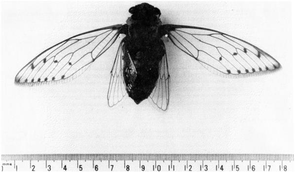
In the tropics, the hot, humid environment is a natural encouragement to growth of all kinds. It is often said that if a walking stick is stuck into the rich fertile soil of the area and left for 3 months, it will sprout leaves and grow. Certainly the insect population reflects this both in size and quantity. Large moths are common to the area and tend to occur in quantity during specific breeding periods. These can quickly cover intake grills, obstructing airflow and even causing large gas turbines to trip. Some of the largest moths are found in the tropics. A common moth in India and Southeast Asia is the Swift moth (Hepralidae), which can have a wing span of some 15 cm and is said to lay up to 1200 eggs in one night. Another moth is the Homoprera shown in Figure 6–1, which has a similar wing span. Moths are attracted by the lights that often surround the turbine installations, as well as the airflow, which acts as a great vacuum cleaner.
On one installation in Sumatra, large gas turbines have been known to trip out after only 8 hours of operation due to blockage of the air filters with moths.
Fortunately, moths tend to confine themselves to within a few miles of land and so offshore installations do not tend to suffer these problems.
Design Problems Experienced
Many feel that standardization is the key to reducing costs and boosting profits. It is not surprising, therefore, that gas turbine air-filter systems were designed with this in mind.
Dust was important to system designers, and so filter systems may be chosen to be able to deal with prodigious amounts of it, whereas, in practice, dust is only normally a problem next to unpaved roads or construction sites.
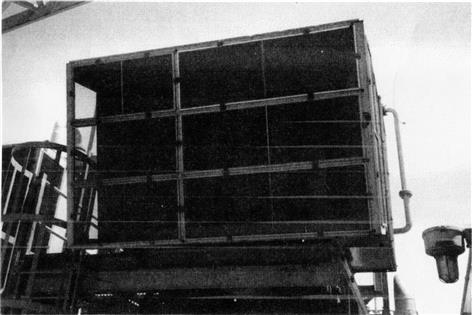
Despite this, most gas turbines were fitted with elaborate and expensive solutions to overcome a problem that hardly existed, or at least only in a relatively small percentage of installations. Many of these systems employ bleed fans that need additional electrical energy and a constant maintenance requirement. A typical system is shown in Figure 6–2. This system employs spin tubes that swirl dust to the outside of the tube where a bleed slot extracts the dust while allowing the cleaner air to pass through the main core of the tube. Since the air is rotated, the peripheral speeds need to be high, which, in turn, results in a relatively high pressure-loss coefficient. The efficiency of the system is very reliant on the bleed air, which is provided by auxiliary fans.
Another bleed extract system uses a series of convergent vanes that funnel the air toward a central slot through which bleed air is extracted. The heavier dust particles are guided toward the bleed extract, while the main air passes between the vanes at almost 180° to the general direction of airflow. Again, the efficiency of the system is reliant on the provision of bleed air.
Protection against rain was elementary. On many systems that had dust-extract systems, no further provision was made. On others a coarse weather louver, often of plastic, was provided. Sometimes a partial weatherhood was provided, sometimes not.
The emphasis on the designer was to provide a “three-stage” filter system, without worrying too much about the suitability of those stages.
There was recognition of the high humidities that exist, and so most systems incorporated a coalescer, whose function was to coalesce small aerosol droplets into larger ones, which could then be drained away. These coalescer panels varied between pieces of knitted mesh wound between bars within the filter housing to separate panels with their own framing. Loose glass fiber pads were used as an inexpensive solution and also served as a prefilter pad.
The final stage in almost all of these systems was the high-efficiency filter element, either as a cartridge or as a bag. The high-efficiency cartridge was typically a deep-pleated glass-fiber paper sealed in its own frame and with a seal on its rear face. Other high-efficiency filters employed glass-fiber pockets that fitted into permanent wire baskets within the filter house.
Almost all of the filter systems were enclosed in housings constructed in carbon steel, finished with a variety of paint finishes. Other materials, such as stainless steel, were not common since their initial cost was thought to be excessive.
Protection against complete filter blockage was often provided by means of a bypass door. This normally was a counterbalanced door in which a weight held the door closed. When the pressure drop across the filter was high, this overcame the force exerted by the balance weight and the door opened, thereby bypassing the filter system with unfiltered air.
Offshore Environment Original Design Data
In Europe in the late 1960s, the only data generally available on the marine environment was generated from that found on ships. Since at that time there was considerable interest in using gas turbines as warship propulsion systems, several attempts were made to define the environment at sea, with particular respect to warships.
Not only was it found difficult to produce consistent data, but other factors such as ship speed, hull design, and height above water level had major effects. It became apparent that predicting salt in air levels was as difficult as predicting weather itself.
Since the gas turbine manufacturers had defined a total limit of the amount of the contaminants that the turbines could tolerate, some definition of the environment was essential to design filter systems that could meet these limits.
Many papers and conferences were held with little agreement, as can be seen in Figure 6–3. However, since the gas turbine industry is a conservative one, it adopted the most pessimistic values as its standard, namely the National Gas Turbine Establishment (NGTE) 30-knot aerosol (Table 6–1). It was treated more as a test standard rather than what its name implied. In the absence of any other data, this was used to define the environment on offshore platforms, despite the fact that they were much higher out of the water, and did not move around at 40 knots!
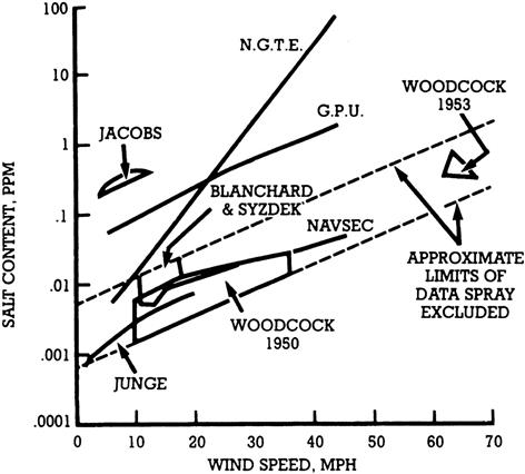
TABLE 6–1
| Microns | Salt Content, ppm |
| <2 | 0.0038 |
| 2–4 | 0.0212 |
| 4–6 | 0.1404 |
| 6–8 | 0.3060 |
| 8–10 | 0.4320 |
| 10–13 | 0.6480 |
| >13 | 2.0486 |
| Total | 3.600 |
(Source: AFI Ltd.)
This then defined the salt in air concentration, but did not address any other particulates. In hindsight, it now seems naive that the offshore environments were originally considered to be clean with no other significant problems than salt. Many equipment specifications were written at that time saying the environment was “dust free.”
In the early 1970s there was also a lively debate as to whether the salt in the air was wet or dry. One argument was put forward that if the salt was wet it would require a further stage of vane separators as the final stage to prevent droplet reentrainment from the filters. The opposing argument maintained that vane separators were unnecessary and that a lower humidity resulted in evaporation of the droplet, giving a smaller salt particle that required a higher degree of filtration. Snow and insect swarms were largely ignored as a problem.
Initial Filter Designs
The types of systems that were used on the first phase of the developments in the North Sea fell into two categories: high-velocity systems where the design face velocity was normally around 6 m/s, and lower velocity systems that operated at 2.5 m/s.
The low-velocity system was a similar system used on land-based installations, and usually comprised a weather louver, followed by a prefilter and a high-efficiency bag or cartridge filter. Sometimes a demister stage was added and occasionally bleed extract inertials were supplied as a first stage.
The high-velocity system was attractive to packagers since it was lighter and occupied a much smaller space. It was the system derived from shipboard use and comprised a vane, coalescer, and vane system.
In general, both systems were housed in mild steel housings with a variety of paint finishes. The weather louvers and vanes were normally constructed from a marine grade aluminum alloy. The filter elements often had stainless steel or galvanized frames.
Bypass doors were used to protect the engine against filter blockage.
The emphasis by package designers was to include a provision for a “three or four stage system” often without regard for what those stages should comprise.
Actual Offshore Environment
The actual offshore environment is in many ways different from that originally envisaged.
Salt in air is present, although it is only a problem when the filtration system leaks or is poorly designed. Horizontal rain can be a severe problem although sea spray does not generally reach the deck levels even in severe storms.
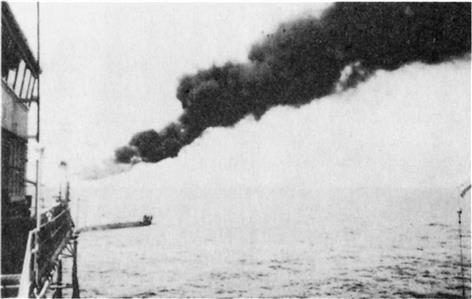
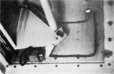
Flare carbon and mud burning can be a significant problem if the flare stack is badly positioned or if the wind changes direction (see Figure 6–4). Not only do the filters block more quickly, but greasy deposits can cover the entire filter system, making the washing of cleanable filters more difficult.
The relative humidity offshore was found to be almost always high enough to ensure that salt was in its wet form. Some splendid work by Tatge, Gordon, and Conkey concluded that salt would stay as supersaturated droplets unless the relative humidity dropped below 45%. Further analysis of offshore humidities in the North Sea showed that this is unlikely to happen (Table 6–2).
TABLE 6–2
Monthly Average Relative Humidity, North Sea
| January | 91 | July | 85 |
| February | 86 | August | 83 |
| March | 87 | September | 83 |
| April | 84 | October | 80 |
| May | 86 | November | 81 |
| June | 84 | December | 80 |
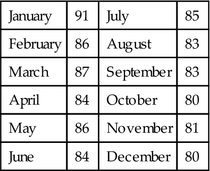
Source: ASME Report 80-GT 174.
Initially it was thought that the platforms were dust free, but this is far from the case.
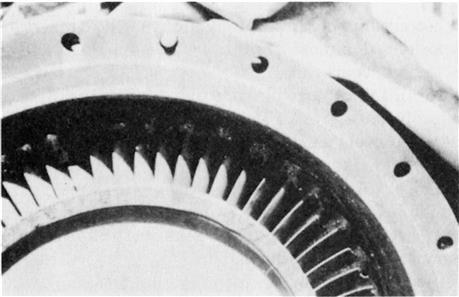
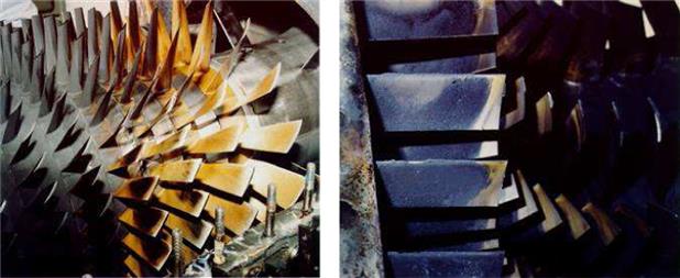
Drilling cement, barytes, and many other dusts are blown around the rig as they are used or moved. But the main problem has resulted from grit blasting. As the platforms got older, repainting was found to be an accelerating requirement with grit blasting a necessary prerequisite.
In order to be effective, grit is sharp and abrasive by design and can be devastating if ingested into a gas turbine (see Figure 6–5). The quantities used can seem enormous. On one platform it was found that over a 12-month period, 700 tons of grit blast had been used!
Offshore Application Design Problems Encountered
In general, problems were slow to appear, typically taking three to five years after start-up, but since a lot of equipment had been installed at about the same time, the problems manifested themselves like an epidemic.
These problems could be categorized as follows:
By far the most serious of these problems was the erosion of compressor blading that was experienced almost simultaneously on many platforms. This occurred about three to five years after start-up, as this was the time that repainting programs were initiated. Grit blast found its way into the turbine intakes either through leaking intakes, bypass doors, or through the media itself (see Figure 6–6). Since the airborne levels were high, the air filters quickly blocked up, allowing the bypass doors to open. As filter maintenance is not a high priority on production platforms, considerable periods were spent with grit passing straight into the turbine through open bypass doors. Even where maintenance standards were more attentive, there were usually enough leaks in the intake housing and ducting to ensure delivery of the grit to the turbine.
It often seemed contradictory that the system designers would spend a lot of time specifying the filter system, but would pay little attention to ensuring the airtightness of the ducting downstream.
Since the grit was sharp, it sometimes damaged the filter media itself, reducing the system efficiency dramatically.
Bypass doors were a major problem. Early designs failed to take account of the environment or the movement in the large structures of the filter housings. Very few of those initial designs were airtight when shut, and it was not uncommon for them to be blown open by the wind.
Turbine corrosion could almost always be traced to leaky ducting or operation with open bypass doors. Very few systems gave turbine corrosion problems if the ducting was airtight. The few installations that did give problems were usually the result of low-velocity systems operating with poor aerodynamics, so that local high velocities reentrained salt water droplets into the airstream and onward to the engine.
Rapid compressor fouling was usually the prelude to more serious problems later, since it was usually caused by the combined problems of filter bypass.
Compressor cleaning almost once a week was fairly standard for systems with those problems.
As time progressed the marine environment took its toll on the carbon steel and severe corrosion was experienced on the intake housing and ducting. In some cases, corrosion debris was ingested into the turbine causing turbine failure. This again was accelerated by poor design, which allowed dissimilar metals to be put into contact, leading to galvanic corrosion.
How Good does your Filter Need to be for the above Applications
The end-user is the best judge of this. Clearly, in the clean air of northern Canada, the gas turbine engine might not be expected to ingest oil fumes (as in offshore applications) or insects (as in the tropics), but icing (ice ingestion) may be a factor. In the heavily industrialized areas of Europe however, dirty particulates are prevalent. The GT system may allow for online washing but some of these particulates bake onto the airfoil surfaces and destroy aerodynamic performance. Additional filtration capacity may be in order, but at what point does the additional capital cost justify itself? What is the GT power that has to be sacrificed for more efficienct filtration and can the end-user tolerate it? These are, once again, end-user questions.
The case study that follows does present some perspective on the testing and financial analysis on three = phase filtration systems. Again, the end-user ought to pay attention to the model numbers of GT involved in this case study and their respective power ratings. Sometimes accessories that work well with one power size bracket of gas turbine may not “scale up” well with larger power brackets due to system geometries, other accessory systems on the gas turbine and various other factors. The study does present the key parameters to be potentially studied were a similar study to be undertaken elsewhere.
Case Study 1: A Test Case of Two- vs. Three-Phase Filtration3
These filtration systems were installed on two Mitsubishi M 701F, two Alstom GT13E2, two GE Frame 9FA, two GE LM 6000, four Solar engines packaged by TurboMach, an Alstom Tempest and two Ruston Typhoons, with corresponding ratings between 4.5 MW and 232 MW, operated at facilities in Singapore, Indonesia, France, Austria, the Netherlands, the UK and Germany. Despite a wide range of different temperatures, humidity levels, dust concentrations, and other local conditions, none of the machines required an online or offline washing routine within an operating period of one year.
High-quality air filters are able to reduce the fouling on the blades and enable stable power output P and efficiency h. Continuous development of filter media and filter construction have improved the filter performance in the past. Will there be further steps towards even better air filtration for gas turbines or has the development reached a plateau? The answer to this question can be found in an economic analysis taking into account a reduction of fouling due to better combustion air quality on the one hand and higher investment costs and higher pressure drop in the air intake on the other hand.
The evaluations and calculations are accomplished at so-called static filter systems where air filters with depth loading characteristics are used. With static filter systems several steps of filtration are arranged in a sequence and therefore the examined upgrades of the filtration efficiencies can be implemented relatively easily so that the effect could be studied. A comparison of two- and three-stage filter systems for intake air filtration at gas turbines produces important findings regarding the most operationally cost-efficient filter sequence overall. The upgrade of the air intake system on the one hand resulted in an increased static pressure loss in the air intake causing reduced turbine efficiency and less power output. On the other hand at the same time the soiling of the blades mainly in the compressor section (compressor fouling) is lowered and as a consequence efficiency and power output are enhanced. The effects of a higher pressure drop entailed by three-stage filtration are compared with those arising from reduced soiling on the blades. In the cases examined, including case studies from actual operation, definite advantages are found for three-stage filtration. Even the modification costs for installing another filter stage can be amortized in what will sometimes be significantly less than two years.
The purity of the combustion air for gas turbines is increasingly a major focus for the manufacturers and operators, since these machines, due to continuous technical design enhancements, are reacting with progressively rising sensitivity to soiling on their blades. Properly functioning filters in the intake air system will reduce soiling on the blades, thus increasing the power output and efficiency of the gas turbine involved. Repeated advances in the fields of filter design and filter media are enhancing the performance capabilities of the air filters being used.
Will the efficiency of the air filters used continue to rise over the years ahead, or has a plateau been reached, and will the future more probably see stagnation at a high level of filtering efficiency? The answer to this question can be supplied only by a feasibility study, in which the advantages of even purer combustion air, and the concomitantly reduced level of blade soiling, are compared to the disadvantages entailed by higher capital investment costs for the intake air system and a higher pressure drop of the filters.
An air filter system is required to significantly reduce the penetration of solid and liquid particles into the turbine under temporally fluctuating environmental conditions. The size of these particles lies within a bandwidth ranging from approx. 0.01 micrometer (μm) to approx. 3 millimeter (mm), thus according to the size ratio between a tennis ball and a 10,000-foot-high mountain. This analogy illustrates why filter systems are often designed in a multi-stage configuration, so as to capture large particles in the pre-filter and small particles in the fine filter.
At a highly polluted location—neglecting extreme situations like sandstorms—the air can be expected to contain average mass concentrations of up to 0.2 mg/mÑ or number concentrations per mÑ of up to 30 million particles of 0.5 μm and larger in size. A gas turbine with an intake volume flow of 1.5 million cubic meters per hour will ingest up to 30 trillion particles of 0.5 μm and larger in size per hour. If a fraction of this dust penetrates the filters, it will either deposit on the blades or cause erosion, leading to reduced power output and impaired efficiency for the gas turbine. The major effects for the deterioration include increased tip clearances, changes in airfoil geometry and increasing surface roughness. In the case of locations near the coast, salt particles being transported in the air may reach the blades, where they cause serious corrosion and consequently shorten the blades’ lifetime quite considerably. The good water solubility of many salts in any case poses tough requirements for the filter system, since water passing through may wash the salts out of the filters again, and transport them into the turbine (see Table 6-3).
TABLE 6–3
Pollution Levels of Ambient Air
| Typical concentration (by mass) of airborne particles in ambient air | 0.01–0.2 mg/m3 |
| Typical concentration (by number) of airborne particles in ambient air | 106–3⋅107 particles/m3 |
| A gas turbine rated at approx. 150 MW ingests approx. 20,000,000,000,000 particles per hour | |
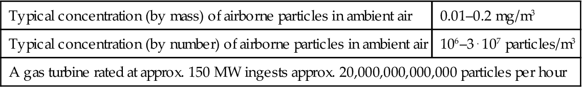
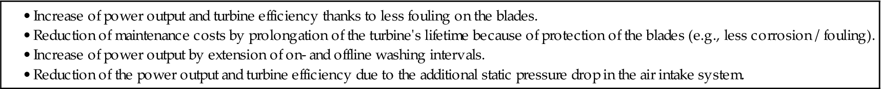
Good air filtration significantly reduces the amount of caked-on dust deposits (fouling) on the blades, thus delaying a temporal fall in the gas turbine’s power output and efficiency. If particles that cause erosion and corrosion are kept away from the gas turbine’s compressor, the blade lifetime will be prolonged. Offline washing for removing caked-on dust particles is one of the substantial cost factors. The washing procedure causes downtimes lasting several hours, during which no power or steam can be generated. In the case of a 150-MW gas turbine, an offline washing routine can mean lost revenues totaling EUR 30,000 to 40,000.
Efficient air filtration is designed to significantly increase the time intervals between two offline washing routines, and thus enable the machine to be run for longer, with a concomitant increase in revenues. The lower costs for any washing agents used, or for fully demineralized washing water for online washing routines should also be mentioned in this context. The overview in Table 6–4 shows the most important beneficial and detrimental influences that combustion air filtration exerts on the operating behavior of gas turbines.
TABLE 6–4
Influences of Intake Air Filtration on Operating Behavior of Gas Turbines
Besides the static filter systems explained in detail below, so-called cleanable filters are also used for filtering the combustion air of gas turbines. The advantages and disadvantages of these filter elements, which operate on the principle of surface filtration and are designed to have the filtered dust removed with a pressure pulse (pulse-jet or pulseclean), have already been discussed elsewhere. Cleanable systems are excluded from the analysis below, and will not be included in the basic analysis (Figure 6.7).
A Comparison of Two- and Three-Stage Filter Systems
From a purely technical point of view, it is definitely possible to reduce the amount of pollutants in the intake air entering a gas turbine, by installing a three-stage filter system with a high-efficiency final filter instead of the two-stage system commonly used today. This would reduce the amount of fouling on the blades; however, the average pressure drop of the filters would rise. In the analysis below, only two of the influencing factors explained above will initially be covered. The first of these is the increase in power output thanks to reduced fouling on the blades, and the second is the countervailing reduced power output due to an increased pressure drop. The criteria under scrutiny, adduced for examining the cost-efficiency of an improved filtration process, are listed below:
1. Increase of the average power output and turbine efficiency due to less fouling on the blades when using a three-stage system.
2. The thereto contrary reduced power output due to the increased pressure drop in the air intake system when using a three-stage system.
Figures 6–8 and 6–9 illustrate the two- and three-stage filter systems being compared, with filter classes defined under EN779: 2003 (coarse and fine dust filters) and EN 1822 (HEPA/ULPA filters) serving as the starting point for assessing the air filter collection efficiency capabilities. For the conventional two-stage filter system, filter classes F6 (pocket filters) and F8 (cassette filters) were selected. This filter combination has proved its worth in many field applications, with useful lifetimes of more than 2 years for both the first and the second filter stages.
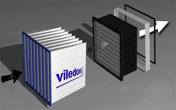
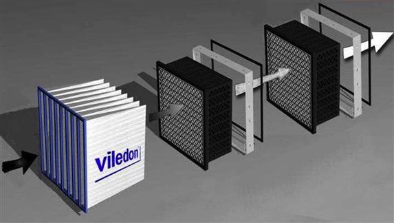
The improvement in filtration is to be effected using the filter sequence F6-F9-H11. The first filter stage, featuring an F6 pocket filter, remains the same compared to the two-stage system, whereas for the second and third filter stages cassette filters of classes F9 and H11 are used. The upgrade job thus involves increasing the number of filter stages from two to three. The first task is to mathematically quantify the adverse effect of the increased pressure drop involved. The causal relationship between pressure drop in the intake system and power output of a gas turbine, as shown in Figure 6–10, is adduced for this purpose; i.e., for each 50 Pa of increased pressure drop the turbine’s power output decreases by 0.1%.
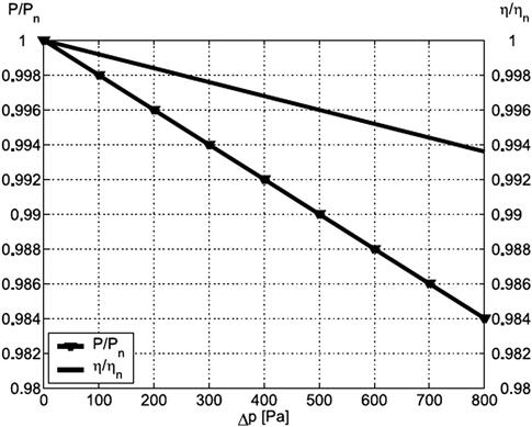
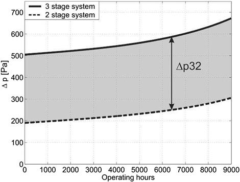
With most gas turbines, the actual value is somewhat smaller than 0.1%, so that the effect of a reduced power output level due to the increased pressure drop tends to be weighted rather more heavily in the calculations below than it actually is. The diagrams in Figures 6–11 and 6–12 show a typical graph for the pressure drops of the above-described two- and three-stage filter systems over the course of 9000 operating hours (approx. 1 year in base-load operation). They are based on the evaluation of monitored pressure drop curves for different machines with two-stage systems and the first installation of a three-stage filtration system.
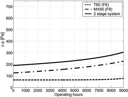
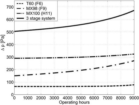
The pressure drop in the air intake system of a gas turbine depends on many factors like, for example, relative humidity, temporarily increased dust concentrations and fluctuating volume flow rate of the turbine. Therefore real life monitored pressure drop curves do not show such a smooth behavior. The average pressure drop curves shown in Figures 6–11 and 6–12 result from flattening out short term fluctuations. The curves marked with “two-stage system” or “three-stage system,” respectively, represent the total pressure drop of the two-stage or three-stage systems. The significantly lower pressure drop in the two-stage filter system can clearly be seen, with the average pressure drop over the entire year being approximately 300 Pa less compared to the three-stage system.
In order to understand the reasons behind the reduced fouling on the blades, the comparison provided in Table 6–5 is helpful. The diagram compares the particle concentrations in the clean air for the two filter sequences F6-F8 and F6-F9-H11, in each case for three particle-size fractions in the as-new condition of the filters. In the F6-F8 two-stage filter system, for example, approx. 7.2 million particles of 0.3–0.5 μm in size still reach the clean-air side of the final filter stage, whereas with the three-stage filter system F6-F9-H11 the figure falls to approx. 0.22 million particles. The filter’s efficiency is approx. 64% in the two-stage configuration compared to 98.9% for the three-stage system; in other words, in comparison to a two-stage system the three-stage filtration holds back approximately 97% of the particles reaching the clean-air side of the final filter stage. This reduced penetration through the filters in a three-stage system is the reason for significantly reduced fouling.
TABLE 6–5
Comparison of the Filter Collection Efficiencies of Two-stage and Three-stage Filter Systems [6-2]
| Particle Size μm | Particles in Atmosphere Number/m3 | Initial Efficiency of Filtration | Particle Penetration Number/m3 | |
| 0.3–0.5 | 20,000,000 | ≈64% | 7,200,000 | 2-stage filtration |
| 0.5–1.0 | 4,000,000 | ≈80% | 800,000 | |
| 1.0–2.0 | 300,000 | ≈95% | 15,000 | |
| 0.3–0.5 | 20,000,000 | ≈98.9% | 220,000 | 3-stage filtration |
| 0.5–1.0 | 4,000,000 | ≈99.9% | 4000 | |
| 1.0–2.0 | 300,000 | ≈99.999% | 3 |
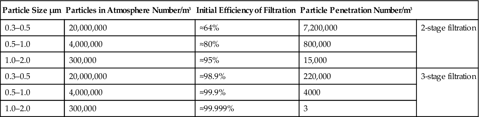
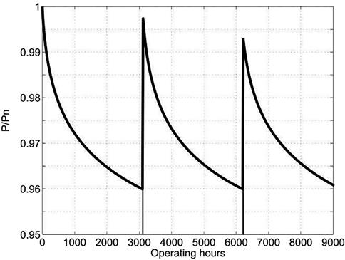
Figure 6–13 shows the typical logarithmic graph for the power output of a gas turbine operated with a two-stage filter system. The graph is based on the evaluation of measured power output data on different machines and the experience of different gas turbine operators concerning the recoverable power output after an offline wash.4 It was assumed that two offline washes per year are performed, so that after approx. 3100 h, the first offline washing routine is carried out, and power output capability is increased. The power output decreases again logarithmically, until after approx. 6200 h another offline washing is performed, and so on. In the case of three-stage filtration with the filter sequence already explained, the decrease in power output is significantly smaller, and the time interval before any washing routine becomes longer (see Figure 6–14).
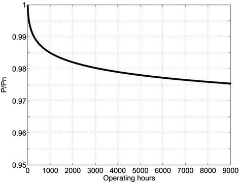
In the example depicted here, taken from actual operation, an offline washing routine was not required within the 9000 operating hours examined. The measured data were approximated by the same logarithmic function as for the two-stage system, but with a new set of coefficients fitting the three-stage system power output (Figures 6–15 to 17).
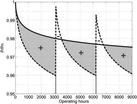
The difference in power output of the gas turbines with two-stage or three-stage systems is calculated each time.5 For the same gas turbine, rated at 165 MW, this means additional energy output of 16,000 MWh over one year. To conclude the analysis, Table 6–6 shows the results of a comparison based on an electricity-generating power plant. For the 165-MW gas turbine, the additional annual revenues are calculated at EUR 189,000. This calculation must be regarded as on the conservative side, given the selling price assumed for electricity, since the revenue for a megawatt-hour of electricity will usually be higher. The decrease of power output for all systems was less than 2%, referenced to the power output in an absolutely clean condition, i.e., the operating behavior observed was more favorable than that depicted in Figure 6–19.
TABLE 6–6
Compilation of the Calculation Results [6-2]
| Less power output due to higher pressure drop | −9700 MWh |
| Higher power output due to less fouling | +16,000 MWh |
| Total gain in power output | +6300 MWh |
| Cost savings @ 30 EUR/MWh @ 40 USD/MWh |
198,000 EUR per annum 252,000 USD per annum |
The useful filter lifetimes for the various filter stages involved, including the Class H11 cassette filters in the third stage, were in all systems longer than one year and reached up to three years. In offline washing routines carried out for trial purposes, the washing water remained clean, and no caked-on deposits of dirt were discernible when the machines were opened up. The above-discussed effects of an improved filtration process have thus all materialized at the 15 test systems, and the calculations can accordingly be verified.
In summary, a comparison of two- and three-stage filter systems for gas turbine intake air filtration reveals important arguments with regard to the most operationally cost-efficient filter sequence overall. The effects of a higher pressure drop entailed by three-stage filtration are compared with those arising from reduced soiling on the blades. In the examined systems, including case studies from actual operation, definite advantages are found for three-stage filtration with the filter sequence F6-F9-H11 in conformity with EN 779 and EN 1822. Even the modification costs for installing another filter stage can be amortized in what will sometimes be significantly less than two years.
Gas Turbine Exhausts6
The gas turbine’s exhaust system conducts the products of combustion—any unburned fuel, excess air, and the heat carried by all these gases—away from the turbine.
In contemporary land-based applications, energy conservation policies, environmental law, and growing awareness of the exhaust steam’s potential resulted in a variety of energy conservation designs that are added to the tail end of the exhaust system. These include mainly (also see Chapters 3 and 10 on gas turbine configurations and heat cycles and efficiency optimization):
• Waste heat steam generation boilers for use in a combined-cycle unit
• Waste heat use for the civilian population’s heating needs (CHPs, combined heat and power plants)
• Waste heat usage for greenhouses that grow vegetables and flowers
By far the most demanding application for exhaust systems is in aircraft engine turbojet applications. In turboprop applications, the bulk of the gas turbine’s power is used to drive the propeller.
This also is the case with land-based power generation where the turbine’s power is being used in part to drive the generator or in land-based mechanical drive where the power turbine uses most of the power generated by the gas generator (the term given to the gas turbine minus the power turbine in mechanical drive application). Much of the turbine module’s power in all applications is used to drive the compressor.
The turbojet application, then, is where the exhaust duct has to withstand the bulk of the gas turbine’s thrust. This is because the exhaust gases exiting the exhaust duct propel the aircraft and its entire payload forward.
The following extract deals with aeroengine exhaust systems. The main difference between aeroengines and nonaeroengines in this respect is the geometry of that section. The aeroengine’s geometry is not configured for transporting exhaust gases to a stack or HRSG. The nonaeroengine’s ducting that conducts the exhaust gases is relatively simple. However, the expansion joints require the most care and cause the most trouble in that area of the gas turbine system. Chapter 8, Accessory Systems, deals with expansion joints.
Aircraft7 gas turbine engines have an exhaust system that passes the turbine discharge gases to atmosphere at a velocity, and in the required direction, to provide the resultant thrust. The velocity and pressure of the exhaust gases create the thrust in the turbo-jet engine but in the turbo-propeller engine only a small amount of thrust is contributed by the exhaust gases, because most of the energy has been absorbed by the turbine for driving the propeller. The design of the exhaust system therefore exerts a considerable influence on the performance of the engine. The areas of the jet pipe and propelling or outlet nozzle affect the turbine entry temperature, the mass airflow and the velocity and pressure of the exhaust jet.
The temperature of the gas entering the exhaust system is between 550 and 850°C according to the type of engine and with the use of afterburning can be 1500°C or higher. Therefore, it is necessary to use materials and a form of construction that will resist distortion and cracking, and prevent heat conduction to the aircraft structure.
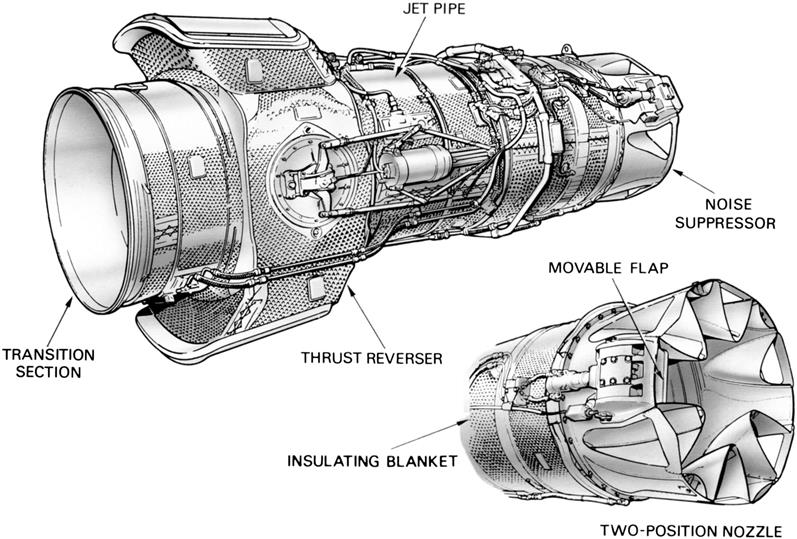
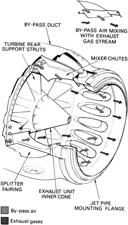
A basic exhaust system is shown in Figure 6–18. The use of a thrust reverser noise suppressor and a two position propelling nozzle entails a more complicated system as shown in Figure 6–19. The low bypass engine may also include a mixer unit (Figure 6–20) to encourage a thorough mixing of the hot and cold gas streams.
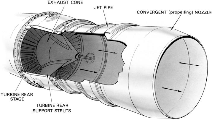
Exhaust Gas Flow
Gas from the engine turbine enters the exhaust system at velocities from 750–1200 feet per second, but, because velocities of this order produce high friction losses, the speed of flow is decreased by diffusion. This is accomplished by having an increasing passage area between the exhaust cone and the outer wall as shown in Figure 6–18. The cone also prevents the exhaust gases from flowing across the rear face of the turbine disc. It is usual to hold the velocity at the exhaust unit outlet to a Mach number of about 0.5, i.e., approximately 950 feet per second. Additional losses occur due to the residual whirl velocity in the gas stream from the turbine. To reduce these losses, the turbine rear struts in the exhaust unit are designed to straighten out the flow before the gases pass into the jet pipe.
The exhaust gases pass to atmosphere through the propelling nozzle, which is a convergent duct, thus increasing the gas velocity. In a turbo-jet engine, the exit velocity of the exhaust gases is subsonic at low thrust conditions only. During most operating conditions, the exit velocity reaches the speed of sound in relation to the exhaust gas temperature and the propelling nozzle is then said to be “choked;” that is, no further increase in velocity can be obtained unless the temperature is increased. As the upstream total pressure is increased above the value at which the propelling nozzle becomes “choked,” the static pressure of the gases at exit increases above atmospheric pressure. This pressure difference across the propelling nozzle gives what is known as “pressure thrust” and is effective over the nozzle exit area. This is additional thrust to that obtained due to the momentum change of the gas stream.
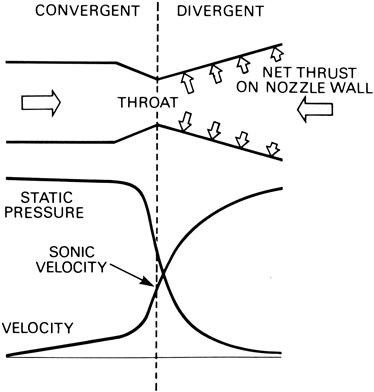
With the convergent type of nozzle wastage of energy occurs, since the gases leaving the exit do not expand rapidly enough to immediately achieve outside air pressure. Depending on the aircraft flight plan, some high-pressure ratio engines can with advantage use a convergent-divergent nozzle to recover some of the wasted energy. This nozzle utilizes the pressure energy to obtain a further increase in gas velocity and, consequently, an increase in thrust.
From the illustration (Figure 6–21), it will be seen that the convergent section exit now becomes the throat with the exit proper now being at the end of the flared divergent section. When the gas enters the convergent section of the nozzle, the gas velocity increases with a corresponding fall in static pressure. The gas velocity at the throat corresponds to the local sonic velocity. As the gas leaves the restriction of the throat and flows into the divergent section, it progressively increases in velocity towards the exit. The reaction to this further increase in momentum is a pressure force acting on the inner wall of the nozzle. A component of this force acting parallel to the longitudinal axis of the nozzle produces the further increase in thrust.
The propelling nozzle size is extremely important and must be designed to obtain the correct balance of pressure, temperature and thrust. With a small nozzle these values increase, but there is a possibility of the engine surging, whereas with a large nozzle the values obtained are too low.
A fixed-area propelling nozzle is only efficient over a narrow range of engine operating conditions. To increase this range, a variable area nozzle may be used. This type of nozzle is usually automatically controlled and is designed to maintain the correct balance of pressure and temperature at all operating conditions. In practice, this system is seldom used as the performance gain is offset by the increase in weight. However, with afterburning a variable area nozzle is necessary.
The bypass engine has two gas streams to eject to atmosphere, the cool bypass airflow and the hot turbine discharge gases.
In a low bypass ratio engine, the two flows are combined by a mixer unit (Figure 6–20) which allows the bypass air to flow into the turbine exhaust gas flow in a manner that ensures thorough mixing of the two streams.
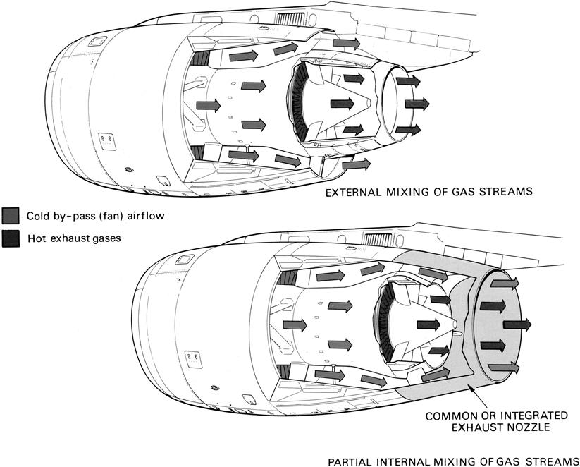
In high bypass ratio engines, the two streams are usually exhausted separately. The hot and cold nozzles are coaxial and the area of each nozzle is designed to obtain maximum efficiency. However, an improvement can be made by combining the two gas flows within a common, or integrated, nozzle assembly. This partially mixes the gas flows prior to ejection to atmosphere. An example of both types of high bypass exhaust system is shown in Figure 6–22.
Construction and Materials
The exhaust system must be capable of withstanding the high gas temperatures and is therefore manufactured from nickel or titanium. It is also necessary to prevent any heat being transferred to the surrounding aircraft structure. This is achieved by passing ventilating air around the jet pipe, or by lagging the section of the exhaust system with an insulating blanket (Figure 6–23). Each blanket has an inner layer of fibrous insulating material contained by an outer skin of thin stainless steel, which is dimpled to increase its strength. In addition, acoustically absorbent materials are sometimes applied to the exhaust system to reduce engine noise.
When the gas temperature is very high (for example, when afterburning is employed), the complete jet pipe is usually of double-wall construction with an annular space between the two walls. The hot gases leaving the propelling nozzle induce, by ejector action, a flow of air through the annular space of the engine nacelle. This flow of air cools the inner wall of the jet pipe and acts as an insulating blanket by reducing the transfer of heat from the inner to the outer wall.
The cone and streamline fairings in the exhaust unit are subjected to the pressure of the exhaust gases; therefore, to prevent any distortion, vent holes are provided to obtain a pressure balance.
The mixer unit used in low bypass ratio engines consists of a number of chutes through which the bypass air flows into the exhaust gases. A bonded honeycomb structure is used for the integrated nozzle assembly of high bypass ratio engines to give lightweight strength to this large component.
Due to the wide variations of temperature to which the exhaust system is subjected, it must be mounted and have its sections joined together in such a manner as to allow for expansion and contraction without distortion or damage.
Gas Turbine Noise Suppression8
With land-based and marine applications, the nature of the application permits the designers to add “houses” around the gas turbine package to provide a measure of noise protection for the personnel working in the area. In applications such as offshore and some naval applications, where weight per delivered unit of horsepower is at a premium, the “house” may be lighter or nonexistent and personnel permanently equipped with hearing protection in the vicinity of the turbine. The design of these protective houses (which also mitigate the risk of explosion) is covered next.
By far the most demanding application for noise mitigation, then, is with aircraft gas turbines. These turbines expose the entire surrounding population on the ground to their noise during takeoff and landing. Tolerant during the Second World War, which accelerated the progress of aircraft gas turbine engines considerably, the public now is extremely demanding, expecting relief from aircraft engine noise.
In all gas turbine applications, the noise one produces is a function of both its aerodynamic design (gas velocity and so forth) and its overall system, which includes its potential for resonance and additional vibration that would not be noted during test cell runs. This would depend on the vibration potential of the gas turbine with:
• Its base mounting in the case of land-based and naval applications
• Its nacelle with aircraft applications
• The entire surrounding mechanical structure, which would include the plant concrete floor, piping, and all other accessories somehow “connected” to the gas turbine via a physical medium in land-based and marine applications
One of the best examples to illustrate this in the case of aeroengines was the following observation (made in the late 1980s) on the early rivalry between the General Electric/Snecma CFM-56 and IAE’s (International Aeroengines) V2500. The first aircraft fitted with the V2500 was the Airbus A321 and the early noise trial records at John Wayne Airport revealed that the V2500 fitted aircraft was not detected by several of the airport’s noise sensors on approach. The same aircraft fitted with CFM-56 engines was observed to “rattle the passenger’s teeth” in a certain range of seat rows. However, all this can change in design development, as designers sort out which component or hardware combination causes the overall result to “rattle” and change it enough to get that configuration to run smoothly.
What follows now is a section on mitigating noise in aircraft engine applications. The reader should note that, for many aircraft engines developed in the days before protecting the public from aircraft engine noise was as high profile as it is today, hush kits with retrofit potential have been developed. A good example is the Pratt and Whitney JT-8D fleet. From the 1950s to the 1980s, this engine’s growth took it from about 9000 pounds of thrust to 19,000 pounds. In the process, it became the world’s largest commercial engine fleet. It no longer is the high-profile engine it once was; however, the number of these engines still out there and operating are legion, particularly in countries that need to buy “bargain used aircraft” from wealthier countries. Retrofit hush kits for these engines (so that they could fly into airports with more stringent noise rules) became popular in the late 1980s.
Airport9 regulations and aircraft noise certification requirements, all of which govern the maximum noise level aircraft are permitted to produce, have made jet engine noise suppression one of the most important fields of research.
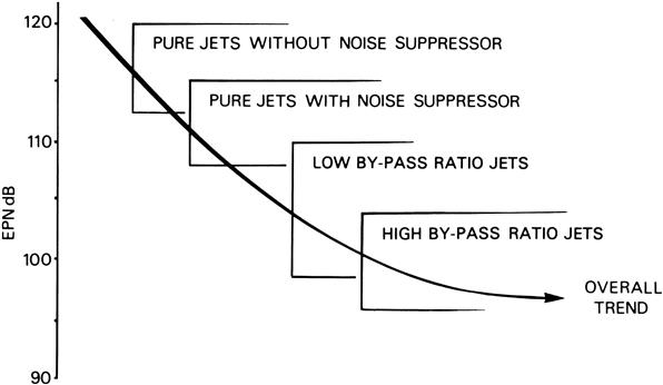
The unit that is commonly used to express noise annoyance is the Effective Perceived Noise deciBel (EPNdB). It takes into account the pitch as well as the sound pressure (decibel) and makes allowance for the duration of an aircraft flyover. Figure 6–24 compares the noise levels of various jet engine types.
Airframe self-generated noise is a factor in an aircraft’s overall noise signature, but the principal noise source is the engine.
To understand the problem of engine noise suppression, it is necessary to have a working knowledge of the noise sources and their relative importance. The significant sources originate in the fan or compressor, the turbine and the exhaust jet or jets. These noise sources obey different laws and mechanisms of generation, but all increase, to a varying degree, with greater relative airflow velocity. Exhaust jet noise varies by a larger factor than the compressor or turbine noise, therefore a reduction in exhaust jet velocity has a stronger influence than an equivalent reduction in compressor and turbine blade speeds.
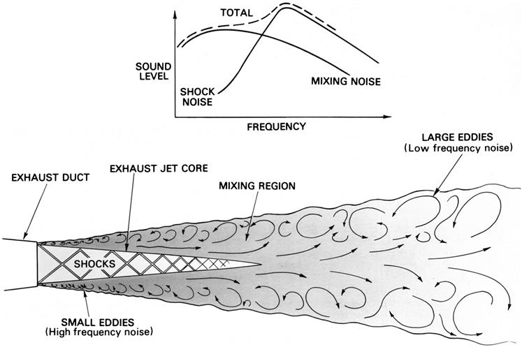
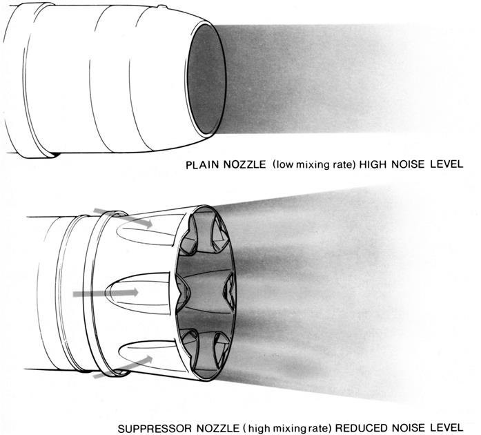
Jet exhaust noise is caused by the violent and hence extremely turbulent mixing of the exhaust gases with the atmosphere and is influenced by the shearing action caused by the relative speed between the exhaust jet and the atmosphere. The small eddies created near the exhaust duct cause high frequency noise but downstream of the exhaust jet the larger eddies create low frequency noise. Additionally, when the exhaust jet velocity exceeds the local speed of sound, a regular shock pattern is formed within the exhaust jet core. This produces a discrete (single frequency) tone and selective amplification of the mixing noise, as shown in Figure 6–24. A reduction in noise level occurs if the mixing rate is accelerated or if the velocity of the exhaust jet relative to the atmosphere is reduced. This can be achieved by changing the pattern of the exhaust jet as shown in Figure 6–25.
Compressor and turbine noise results from the interaction of pressure fields and turbulent wakes from rotating blades and stationary vanes, and can be defined as two distinct types of noise; discrete tone (single frequency) and broadband (a wide range of frequencies). Discrete tones are produced by the regular passage of blade wakes over the stages downstream causing a series of tones and harmonics from each stage. The wake intensity is largely dependent upon the distance between the rows of blades and vanes. If the distance is short then there is an intense pressure field interaction, which results in a strong tone being generated. With the high bypass engine, the low pressure compressor (fan) blade wakes passing over downstream vanes produce such tones, but of a lower intensity due to lower velocities and larger blade/vane separations. Broadband noise is produced by the reaction of each blade to the passage of air over its surface, even with a smooth airstream. Turbulence in the airstream passing over the blades increases the intensity of the broadband noise and can also induce tones.
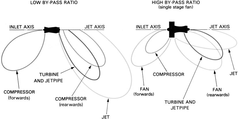
With the pure jet engine the exhaust jet noise is of such a high level that the turbine and compressor noise is insignificant at all operating conditions, except low landing-approach thrusts. With the bypass principle, the exhaust jet noise drops as the velocity of the exhaust is reduced but the low pressure compressor and turbine noise increases due to the greater internal power handling. The introduction of a single-stage low-pressure compressor (fan) significantly reduces the compressor noise because the overall turbulence and interaction levels are diminished. When the bypass ratio is in excess of approximately 5 to 1, the jet exhaust noise has reduced to such a level that the increased internal noise source is predominant. A comparison between low and high bypass engine noise sources is shown in Figure 6–26.
Listed amongst the several other sources of noise within the engine is the combustion chamber. It is a significant but not a predominant source, due in part to the fact that it is “buried” in the core of the engine. Nevertheless it contributes to the broadband noise, as a result of the violent activities that occur within the combustion chamber.
Methods of Suppressing Noise
Noise suppression of internal sources is approached in two ways; by basic design to minimize noise originating within or propagating from the engine, and by the use of acoustically absorbent linings. Noise can be minimized by reducing airflow disruption, which causes turbulence. This is achieved by using minimal rotational and airflow velocities and reducing the wake intensity by appropriate spacing between the blades and vanes. The ratio between the number of rotating blades and stationary vanes can also be advantageously employed to contain noise within the engine.
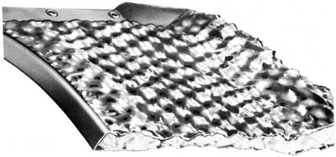
As previously described, the major source of noise on the pure jet engine and low bypass engine is the exhaust jet, and this can be reduced by inducing a rapid or shorter mixing region. This reduces the low frequency noise but may increase the high frequency level. Fortunately, high frequencies are quickly absorbed in the atmosphere and some of the noise that does propagate to the listener is beyond the audible range, thus giving the perception of a quieter engine. This is achieved by increasing the contact area of the atmosphere with the exhaust gas stream by using a propelling nozzle incorporating a corrugated or lobe-type noise suppressor (Figure 6–27).
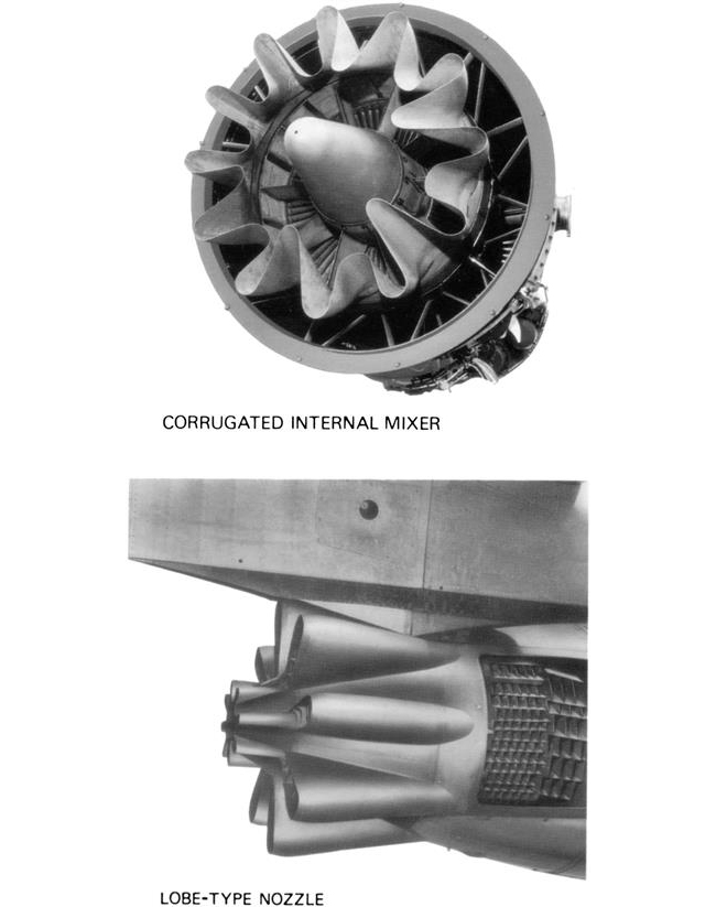
In the corrugated nozzle, free stream atmospheric air flows down the outside corrugations and into the exhaust jet to promote rapid mixing. In the lobe-type nozzle, the exhaust gases are divided to flow through the lobes and a small central nozzle. This forms a number of separate exhaust jets that rapidly mix with the air entrained by the suppressor lobes. This principle can be extended by the use of a series of tubes to give the same overall area as the basic circular nozzle.
Deep corrugations, lobes, or multi-tubes give the largest noise reductions, but the performance penalties incurred limit the depth of the corrugations or lobes and the number of tubes. For instance, to achieve the required nozzle area, the overall diameter of the suppressor may have to be increased by so much that excessive drag and weight results. A compromise that gives a noticeable reduction in noise level with the least sacrifice of engine thrust, fuel consumption, or addition of weight is therefore the designer’s aim. The high bypass engine has two exhaust streams to eject to atmosphere. However, the principle of jet exhaust noise reduction is the same as for the pure or low bypass engine, i.e., minimize the exhaust jet velocity within overall performance objectives. High bypass engines inherently have a lower exhaust jet velocity than any other type of gas turbine, thus leading to a quieter engine, but further noise reduction is often desirable. The most successful method used on bypass engines is to mix the hot and cold exhaust streams within the confines of the engine (Figure 6–27) and expel the lower velocity exhaust gas flow through a single nozzle.
In the high bypass ratio engine the predominant sources governing the overall noise level are the fan and turbine. Research has produced a good understanding of the mechanisms of noise generation and comprehensive noise design rules exist. As previously indicated, these are founded on the need to minimize turbulence levels in the airflow, reduce the strength of interactions between rotating blades and stationary vanes, and the optimum use of acoustically absorbent linings.
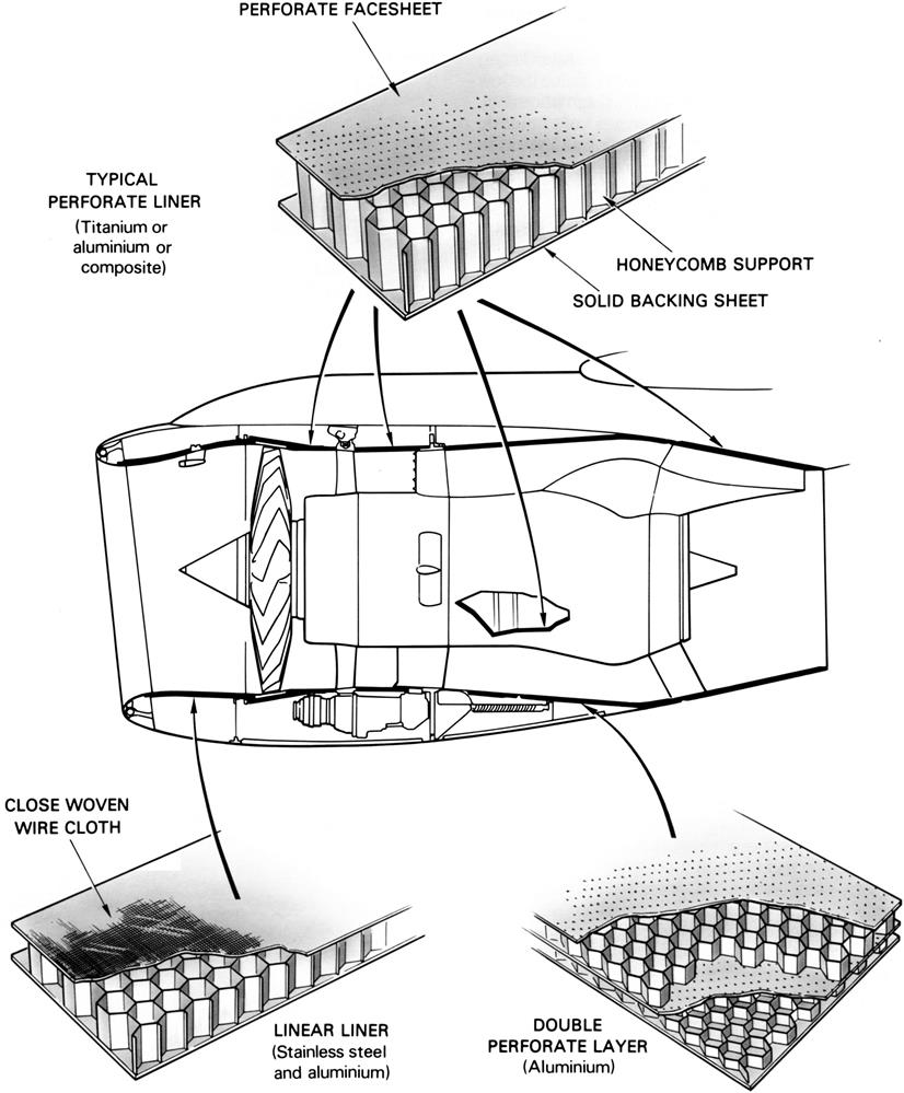
Noise absorbing “lining” material converts acoustic energy into heat. The absorbent linings (Figure 6–28) normally consist of a porous skin supported by a honeycomb backing, to provide the required separation between the facesheet and the solid engine duct. The acoustic properties of the skin and the liner depth are carefully matched to the character of the noise, for optimum suppression. The disadvantage of liners is the slight increase in weight and skin friction and hence a slight increase in fuel consumption. They do, however, provide a very powerful suppression technique.
Construction and Materials
The corrugated or lobe-type noise suppressor forms the exhaust propelling nozzle and is usually a separate assembly bolted to the jet pipe. Provision is usually made to adjust the nozzle area so that it can be accurately calibrated. Guide vanes are fitted to the lobe-type suppressor to prevent excessive losses by guiding the exhaust gas smoothly through the lobes to atmosphere. The suppressor is a fabricated welded structure and is manufactured from heat-resistant alloys.
Various noise absorbing lining materials are used on jet engines. They fall mainly within two categories, lightweight composite materials that are used in the lower temperature regions and fibrous-metallic materials that are used in the higher temperature regions. The noise absorbing material consists of a perforate metal or composite facing skin, supported by a honeycomb structure on a solid backing skin, which is bonded to the parent metal of the duct or casing.
Nonaeroengine (Land-Based) Gas Turbine Noise Suppression10
Nonaeroengines generally have a “turbine house” around their main modules and systems.
Enclosures around noisy rotating machinery, particularly gas turbines, provide protection against noise and help contain risk from situations such as small gas leaks. The design of acoustic gas turbine enclosures is summarized in this section in text extracts from two papers on the subject. These extracts give the reader all the salient points to watch for if specifying or buying an acoustic enclosure. It also provides the reader with basic knowledge of how acoustic sound intensity measurements are conducted generally (i.e., for any kind of equipment). Note also that these designs were built for offshore applications where weight has to be minimized.
Applications of Sound Intensity Measurements to Gas Turbine Engineering
A = total absorption in receiving room
L1, L2 = sound pressure levels, dB
LI = sound intensity level, dB
Gas turbines that are supplied to the oil and power industries are usually given extensive acoustic treatment to reduce the inherent high noise levels to acceptable limits. The cost of this treatment may be a significant proportion of the total cost of the gas turbine installation. In the past it has been difficult to determine if the acoustic treatment is achieving the required noise limits because of a number of operational problems. These problems include: the presence of other nearby, noisy equipment, the influence of the environment, and instrumentation limitations. Traditionally, sound measurements have been taken using a sound level meter that responds to the total sound pressure at the microphone irrespective of the origin of the sound. So, the enforcement of noise limits has been difficult because of uncertainties concerning the origin of the noise.
Recent advances in signal processing techniques have led to the development of sound intensity meters that can determine the direction, as well as the magnitude, of the sound, without the need for expensive test facilities. These instruments enable the engineer to determine if large equipment, such as gas turbine packages, meet the required noise specification even when tested in the factory or on site where other noise sources are present.
There are, of course, limitations in the use of sound intensity meters, and there are some differences of opinion on measurement techniques. Nevertheless, the acoustic engineer’s ability to measure and identify the noise from specific noise sources has been greatly enhanced.
In this section, the differences between sound pressure, sound intensity, and sound power are explained. Measurement techniques are discussed with particular references to the various guidance documents that have been issued. Some case histories of the use of sound intensity meters are presented that include field and laboratory studies relating to gas turbines and other branches of industry.
Sound Fundamental Concepts
Sound Pressure, Sound Intensity, and Sound Power
Any item of equipment that generates noise radiates acoustic energy. The total amount of acoustic energy it radiates is the sound power. This is, generally, independent of the environment. What the listener perceives is the sound pressure acting on his or her eardrums and it is this parameter that determines the damaging potential of the sound. Unlike the sound power, the sound pressure is very dependent on the environment and the distance from the noise source to the listener.
Traditional acoustic instrumentation, such as sound level meters, detects the sound pressure using a single microphone that responds to the pressure fluctuations incident upon the microphone. Since pressure is a scalar quantity, there is no simple and accurate way that such instrumentation can determine the amount of sound energy radiated by a large source unless the source is tested in a specially built room, such as an echoic or reverberation room, or in the open air away from sound reflecting surfaces. This imposes severe limitations on the usefulness of sound pressure level measurements taken near large equipment that cannot be moved to special acoustic rooms.
Sound intensity is the amount of sound energy radiated per second through a unit area. If a hypothetical surface, or envelope, is fitted around the noise source, then the sound intensity is the number of acoustic watts of energy passing through 1 m of this envelope (see Figure 6–29). The sound intensity, I, normal to the spherical envelope of radius, r, centered on a sound source of acoustic power, W, is given by
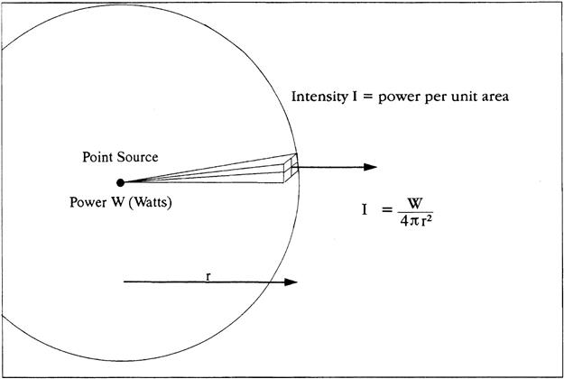
Clearly, the total sound power is the product of the sound intensity and the total area of the envelope if the sound source radiates uniformly in all directions. Since the intensity is inversely proportional to the distance of the envelope from the noise source, the intensity diminishes as the radius of the envelope increases. But as this distance increases, the total area of the envelope increases also, so the product of the intensity and the surface area (equal to the sound power) remains constant.
When a particle of air is displaced from its mean position by a sound wave that is moving through the air there is a temporary increase in pressure. The fact that the air particle has been displaced means that it has velocity. The product of the pressure and the particle velocity is the sound intensity. Since velocity is a vector quantity, so is sound intensity. This means that sound intensity has both direction and magnitude.
It is important to realize that sound intensity is the time-averaged rate of energy flow per unit area. If equal amounts of acoustic energy flow in opposite directions through a hypothetical surface at the same time, then the net intensity at that surface is zero.
Reference Levels
Most parameters used in acoustics are expressed in decibels because of the enormous range of absolute levels normally considered. The range of sound pressures that the ear can tolerate is from 2 × 10⁻⁵ Pa to 200 Pa. This range is reduced to a manageable size by expressing it in decibels, and is equal to 140 dB.
The sound pressure level (SPL) is defined as
Likewise, sound intensity level (SIL) and sound power level (PWL) are normally expressed in decibels. In this case,
The Relationship between Sound Pressure Level and Sound Intensity Level
When the sound intensity level is measured in a free field in air, then the sound pressure level and sound intensity level in the direction of propagation are numerically the same. In practice most measurements of the sound intensity are not carried out in a free field, in which case there will be a difference between the sound pressure and intensity levels. This difference is an important quantity and is known by several terms, such as reactivity index, pressure-intensity index, P-I index, phase index, or LK value. This index is used as a “field indicator” to assess the integrity of a measurement in terms of grades of accuracy or confidence limits. This will be considered in more detail later in this section.
Instrumentation
Sound Intensity Meters
A sound intensity meter comprises a probe and an analyzer. The analyzer may be of the analog, digital, or FFT (fast Fourier transform) type. The analog type has many practical disadvantages that make it suitable only for surveys and not precision work.
Digital analyzers normally display the results in octave or ⅓ octave frequency bands. They are well suited to detailed investigations of noise sources in the laboratory or on site. Early models tended to be large and heavy and require electrical main supplies, but the latest models are much more suited to site investigations.
FFT analyzers generate spectral lines on a screen. This can make the display very difficult to interpret during survey sweeps because of the amount of detail presented. Another disadvantage of FFT-based systems is that their resolution is generally inadequate for the synthesis of ⅓ octave band spectra.
Sound Intensity Probes
There are several probe designs that employ either a number of pressure microphones in various configurations or a combination of a pressure microphone and a particle velocity detector. The first type of probe uses nominally identical pressure transducers that are placed close together. Various arrangements have been used with the microphones either side by side, face to face, or back to back. Each configuration has its own advantages and disadvantages.
If the output signals of two microphones are given by Pa and Pb, then the average pressure, P, between the two microphones is
(6.2)
The particle velocity, u, is derived from the pressure gradient between the two microphones by the relationship
(6.3)
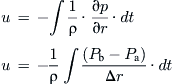 (6.3)
(6.3)Since sound intensity, I, is the product of the pressure and particle velocity, combining equations (6.2) and (6.3) gives the intensity as
(6.4)
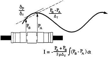
Figure 6–30 shows a two-microphone probe, with a face-to-face arrangement, aligned parallel to a sound field. In this orientation the pressure difference is maximized, and so is the intensity. If the probe is aligned so that the axis of the two microphones is normal to the direction of propagation of the sound wave, then the outputs of the two microphones would be identical in magnitude and phase. Since the particle velocity is related to the difference between the two pressures, Pa and Pb, then the intensity would be zero.
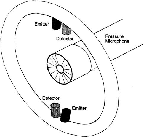
The second type of probe combines a microphone, to measure the pressure, and an ultrasonic particle velocity transducer. Two parallel ultrasonic beams are sent in opposite directions as shown in Figure 6–31. The oscillatory motion of the air caused by audio-frequency sound waves produces a phase difference between the two ultrasonic waves at their respective detectors. This phase difference is related to the particle velocity component in the direction of the beams. This measure of particle velocity is multiplied directly by the pressure to give the sound intensity.
Guidelines and Standards in Sound Intensity Measurements and Measurement Technique
Guidelines and Standards
Work began in 1983 on the development of an international standard on the use of sound intensity and the final document is about to be issued. Further standards are expected dealing specifically with instrumentation.
In the absence of a full standard the only guidance available was the draft ISO standard (ISO/DP 9614) and a proposed Scandinavian standard (DS F88/146).
The ISO document ISO/DP 9614 gives specific methods for determining the sound power levels of noise sources within specific ranges of uncertainty.
The proposed test conditions are less restrictive than those required by the International Standards series ISO 3740–3747, which are based on sound pressure measurements. The proposed standard is based on the sampling of the intensity normal to a measurement surface at discrete points on this surface. The method can be applied to most noise sources that emit noise that is stationary in time and it does not require special purpose test environments.
The draft document defines three grades of accuracy with specified levels of uncertainty for each grade. Since the level of uncertainty in the measurements is related to the source noise field, the background noise field, and the sampling and measurement procedures, initial procedures are proposed that determine the accuracy of the measurements. These procedures evaluate the “field indicators” that indicate the quality of the sound power measurements. These field indicators consider, among other things:
• The pressure–intensity index (or reactivity index)
• The variation of the normal sound intensities over the range of the measurement points
• The temporal variation of the pressure level at certain monitoring points
The three grades of measurement accuracy specified in ISO/DP 9614, and the associated levels of uncertainty, are given in Table 6–7.
TABLE 6–7
Uncertainty of the Determination of Sound Power Level (ISO/DP 9614)
| Octave Band Center Frequencies, Hz | ⅓ Octave Band Center Frequencies, Hz | Standard Deviations, dB | ||
| Class 1 | Class 2 | Class 3 | ||
| 63–125 | 50–160 | 2 | 3 | 4 |
| 250–500 | 200–630 | 1.5 | 2 | 4 |
| 1000–4000 | 800–5000 | 1 | 1.5 | 4 |
| 6300 | 2 | 2.5 | 4 | |
| A Weighted 160–6300 Hz | 1 | 1.5 | 4 | |
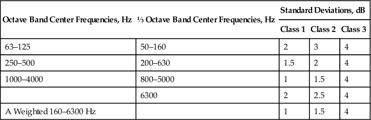
1Class 1 = Precision Grade, Class 2 = Engineering Grade, Class 3 = Survey Grade.
2The width of the 95% confidence intervals corresponds approximately to four times the dB values in this table.
(Source: AFI Ltd.)
The Scandinavian proposed standard DSF 88/146 was developed for the determination of the sound power of a sound source under its normal operating conditions and in situ. The method uses the scanning technique whereby the intensity probe is moved slowly over a defined surface while the signal analyzer time-averages the measured quantity during the scanning period.
The results of a series of field trials by several Scandinavian organizations suggested that the accuracy of this proposed standard is compatible with the “Engineering Grade,” as defined in the ISO 3740 series.
The equipment under test is divided into a convenient number of subareas that are selected to enable a well-controlled probe sweep over the subarea. Guidance is given on the sweep rate and the line density. Measurement accuracy is graded according to the global pressure-intensity index, LK. This is the numerical difference between the sound intensity level and the sound pressure level. If this field indicator is less than or equal to 10 dB then the results are considered to meet the engineering grade of measurement accuracy. As this field indicator increases in value, the level of uncertainty in the intensity measurement increases. When the LK value lies between 10 and 15 dB the measurement accuracy meets the “Survey” grade.
Measurement Techniques
The precise measurement technique adopted in a particular situation depends on the objectives of the investigation and the level of measurement uncertainty that is required.
Subareas
It was mentioned earlier that the total sound power is the product of the intensity and the surface area of the measurement envelope around the noise source. In practice, most noise sources do not radiate energy uniformly in all directions so it is good practice to divide the sound source envelope into several subareas. Each subarea is then assessed separately, taking into account its area and the corresponding intensity level. The subarea sound powers can then be combined to give the total sound power of the source.
The number, shape, and size of each subarea are normally dictated by two considerations: the physical shape of the source and the variations in intensity over the complete envelope. Subareas are normally selected to conform to components of the whole source such that the intensity over the subarea is reasonably constant. It is important that the subareas are contiguous and the measurement envelope totally encloses the source under investigation.
Sweep or Point Measurement
Should one measure the intensity levels at discrete positions, with the probe stationary, or should the probe be swept over the subarea? This controversy has occupied much discussion time among practicing acousticians. For precision grade measurements, discrete points are used, but for lower grade work, sweeping is acceptable.
If discrete points are used then the number and distribution of the measurement points must be considered in relation to the field indicators.
In surroundings that are not highly reverberant and where extraneous noise levels are lower than the levels from the source under investigation, relatively few discrete points may be used, distributed uniformly over the surface. The distance from the source may be as great as 1 m.
As the extraneous noise levels increase and/or the environment becomes more reverberant, measurements must be made progressively closer to the source in order to maintain an acceptable level of uncertainty in the measurements. This also requires more measurement points to be used because of the increase in the spatial variation of the intensity distribution.
If sweeping is used then other factors must also be considered. The speed with which the probe is swept across the subarea must be uniform, at about 300 mm/sec, and the area should be covered by a whole number of sweeps with an equal separation between sweep lines. Care must be taken that excessive dwell time does not occur at the edges of the subarea when the probe’s direction of sweep is reversed. The operator must also be careful that his or her body does not influence the measurements by obscuring sound entering the measurement area as he or she sweeps.
Distance between Source and Probe
Generally, the greater the extraneous noise and the more reverberant the environment then the closer should be the probe to the source. In extreme cases the probe may be only a few centimeters from the source surface in order to improve the signal-to-noise ratio. This is normally frowned upon when using conventional sound level meters because measurements of sound pressure, taken close to a surface, may bear little relation to the pressures occurring further away from the surface. This discrepancy is not due simply to the attenuation with distance that normally occurs in acoustics.
The region very close to a surface is called the “near field.” In this region the local variations in sound pressure may be very complex because some of the sound energy may circulate within this near field and not escape to the “far field.” This recirculating energy is known as the reactive sound field. The sound energy that does propagate away from the surface is called the active sound field because this is the component that is responsible for the acoustic energy in the far field.
Since sound intensity meters can differentiate between the active and reactive sound fields, measurements of intensity taken close to noise sources can faithfully indicate the radiated sound energy. However, using a conventional sound level meter near to a noise source may indicate higher sound power levels than occur in the far field because these instruments cannot differentiate between active and reactive fields.
Some Advantages and Limitations in Sound Intensity Measurements
Background Noise
One of the main advantages of the sound intensity method of measurement is that accurate assessments of sound power can be made even in relatively high levels of background noise. But this is only true if the background noise is steady (i.e., not time varying). Using conventional sound pressure level methods the background noise level should be 10 dB below the signal level of interest.
Using sound intensity techniques the sound power of a source can be measured to an accuracy of 1 dB even when the background noise is 10 dB higher than the source noise of interest. Figure 6–32(a) shows a noisy machine enclosed by a measurement surface. If the background noise is steady, and there is no sound absorption within the measurement surface, then the total sound power emitted by the machine will pass through the measurement surface, as shown.

If, however, the noisy machine is outside the measurement surface, as shown in Figure 6–32(b), then the sound energy flowing into the surface on the left hand side will be emitted from the right hand side of the measurement surface. When the sound intensity is assessed over the whole measurement surface the net sound power radiated from the total surface will be zero.
Effects of the Environment
When the sound power of a noise source is evaluated in the field using sound pressure level techniques, it is necessary to apply a correction to the measured levels to account for the effects of the environment. This environmental correction accounts for the influence of undesired sound reflections from room boundaries and nearby objects.
Since a sound intensity survey sums the energy over a closed measurement surface centered on the source of interest, the effects of the environment are cancelled out in the summation process in the same way that background noise is eliminated. This means that, within reasonable limits, sound power measurements can be made in the normal operating environment even when the machine under investigation is surrounded by similar machines that are also operating.
Sound Source Location
Since a sound intensity probe has strong directional characteristics there is a plane at 90° to the axis of the probe in which the probe is very insensitive. A sound source just forward of this plane will indicate positive intensity, whereas if it is just behind this plane the intensity will be negative (Figure 6–33).
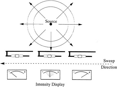
This property of the probe can be used to identify noise sources in many practical situations. The normal procedure is to perform an initial survey of the noise source to determine its total sound power. The probe is pointed toward the source system to identify areas of high sound intensity. Then the probe is reoriented to lie parallel to the measurement surface and the scan is repeated. As the probe moves across a dominant source the intensity vector will flip to the opposite direction.
Testing of Panels
The traditional procedure for measuring the transmission loss, or sound reduction index, of building components is described in the series of standards ISO 140. The test method requires the panel under investigation to be placed in an opening between two independent, structurally isolated reverberation rooms, as shown in Figure 6–34.
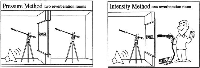
Sound is generated in the left hand room and the sound pressure levels in the two rooms are measured. Assuming that the sound energy in the right hand room comes through the panel then the sound reduction index (SRI) of the panel is given by
(6.5)
For this method to give accurate results, flanking transmission (sound bypassing the test panel) must be minimal and both rooms must be highly reverberant.
If the measurements in the right hand room are carried out using sound intensity, then it is necessary to reduce the amount of reverberation in this room. Since the probe can measure the sound intensity coming through the panel then flanking transmission is no longer a limitation.
For these reasons one can dispense with the second reverberation room altogether. The sound reduction index is then given by
(6.6)
If the panel contains a weak area, such as a window, the sound reduction index of the window can be assessed separately. But this will only work if the panel is a greater sound insulator than the window.
Measuring Tonal Noise Sources
Measuring the sound power of tonal noise sources presents difficulties using traditional techniques (ISO 3740, 1980). Unfortunately, using sound intensity techniques on such sources is also fraught with problems. This is because the spatial distribution of the intensity is very sensitive to small alterations in source position and the presence of nearby sound reflective objects.
Case Study 2: The Use of Sound Intensity Measurement
Gas Turbine Package Witness Testing
Gas turbine packages are normally assembled in large factory buildings or in the open air between factory buildings. In either case, the environment is totally unsuitable for reliable acoustic tests to be carried out using sound level meters alone. Sound intensity techniques are especially relevant in these situations because of the location in which the tests are to be carried out and because some components, such as the compressor test loop, may not be contract items. By surveying each component with a sound intensity meter the sound power for each component can be determined separately.
Figure 6–35 shows a typical gas turbine driving a compressor. The figures on the drawing indicate the sound pressure and sound intensity levels that were measured during a particular witness test on an RB211 gas turbine package. The sound pressure levels in close proximity to the package were between 89 and 103 dB(A), with the higher levels dominating. Even so, reliable values of the intensity levels were obtained from which the sound power levels were determined. These values are given in Table 6–8. Since the sound intensity level is numerically equal to the sound pressure level in free field, the average sound intensity over a given surface area of a gas turbine package provides a direct indication of the average sound pressure level from that surface in free field conditions.
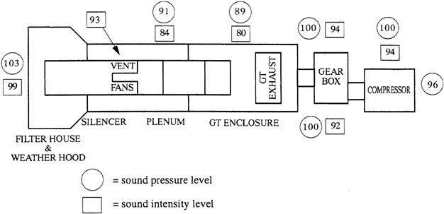
TABLE 6–8
Rank Ordering of Components in Terms of the A-Weighted Sound Power Levels
| Description of Measured Item | Measured Sound Power Levels, dB(A) |
| Combustion air intake | 110 |
| Composition air plenum and silencer | 104 |
| Turbine comp. vent, air breakout | 104 |
| Turbine enclosure | 103 |
| Compressor casing | 103 |
| Gearbox | 103 |
| Breakout from temporary exhaust | 96 |
(Source: AFI Ltd.)
Referring again to Figure 6–35, the sound intensity level measured by the casing of the ventilation fan was 94 dB(A). It would not normally be possible to measure the output from this fan accurately, using a sound level meter, in this situation because of the relatively high sound pressure level in this area due to other sources.
During the testing of another package, the sound power levels from the ventilation fan casing and the fan motor were measured separately. The fan motor was found to be noisier than the manufacturer’s stated levels. Discussions with the motor manufacturer revealed that the wrong cooling fans had been fitted to the motors, which accounted for this increase in noise level. The correct cooling fans were subsequently fitted.
This example clearly illustrates the benefits of sound intensity measurements to check compliance with noise specifications when the test items are very large and are cited in acoustically undesirable areas.
Case Study 3: Comparison of Noise on Two Nominally Identical Production Machines
This example is taken from an extensive survey of a production department that had many, relatively small, machines close together in a highly reverberant factory room. The two machines were nominally identical roller mills, as used in many production lines in the paint, flour, and confectionary industries. The drive motors were situated on the top of the machines. A routine sound intensity survey was carried out on each machine during normal production because it was not possible to run the machines in isolation. The two machines are identified as machine A and machine B.
Table 6–9 gives the overall, A-weighted sound pressure levels and sound power levels for each machine, and the sound power levels of the motors. The total sound power levels of the machines agreed very well with the values obtained by the manufacturer using sound pressure measurements to derive the sound power levels (ISO 3740, 1980). This technique can only give the total sound power of a machine; it cannot obtain the sound power levels of parts of a machine.
TABLE 6–9
Comparison of the Sound Levels from Two Roller Mills
| Description | Machine A, dB(A) | Machine B, dB(A) |
| Total sound power for machine | 96 | 94 |
| Sound pressure level by machine | 92 | 89 |
| Sound power level of the motor | 93 | 85 |
(Source: AFI Ltd.)
At the time of the survey two machines were each in areas of high noise levels and their total sound power levels were 96 and 94 dB(A). But comparing the motor sound power levels revealed a difference of 8 dB(A) in their respective levels even though both motors were classified as the “low noise” type and cost more than the standard motors. This is just one example where a significant degree of noise control might be achievable by selecting the correct one of two nominally identical electric motors. However, using the traditional method of sound pressure level measurement would not reveal any difference between the motors.
Acoustical Properties of Flexible Connectors
Heavy-duty flexible connectors are used to join separate components of a gas turbine package. When high-performance acoustic hardware is used it is imperative that these flexible connectors do not compromise the total acoustic performance of the package. This is particularly so in the gas turbine exhaust system where multilayered flexible connectors are exposed to high temperatures and severe buffeting from exhaust gases. In some exhaust systems overlapping metal plates are inserted inside the flexible connectors to reduce the buffeting of the flexible material. If additional sound attenuation is required, a heavy, fibrous mat, or “bolster,” is inserted between the plates and the flexible connector.
For the acoustics engineer, these flexible connectors are a problem because there are very few data on their acoustical performance, and the designs do not lend themselves to simple theoretical prediction. A brief laboratory investigation was carried out to compare the performances of seven types of flexible connectors with and without plates and bolsters. The tests were carried out in Altair’s acoustical laboratory, which was designed to test materials using sound intensity techniques. The samples were physically quite small so the low-frequency performances were probably distorted by the small size of the samples. Nevertheless, the exercise yielded much valuable information and led to a simple engineering method of predicting a flexible connector’s acoustic performance from knowledge of its basic parameters.
Figure 6–36 compares the sound reduction indices of a typical, multilayered flexible connector tested alone, with plates and with bolster and plates. All of the test results showed a sharp increase in performance at 250 Hz due to the plates. No satisfactory explanation can be offered at this stage for this effect, which may be related to the small size of the samples. But in the middle and high frequencies the results were generally as expected with the plate giving an additional attenuation of about 5 dB compared to the compensator alone. The combination of the plate and bolster gave an additional attenuation of between 10 and 15 dB compared to the flexible connector alone.
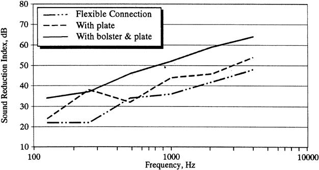
Sound Source Location
During two noise surveys the sound power levels from two different designs of lube oil console were measured using the sound intensity meter. The overall sound power levels were 93 dB(A) and 109 dB(A). The two consoles had electrically driven pumps and both emitted strong tonal noise. In the first case the tonal noise was centered on 8 kHz; using the sound intensity probe it was possible to “home in” on the pump section pipe as a major noise source. This was confirmed by vibration measurements.
In the second survey the pump outlet pipe gave the highest sound intensity reading. Since this was a relatively long pipe, which was rigidly attached to the frame of the console, it was a dominant source both in its own right and because it was “exciting” the framework. In these cases the sound intensity meter was a useful tool in identifying dominant sources among a number of small, closely packed noise radiators.
This section has discussed the concepts of sound intensity, sound power, and sound pressure. It has shown how sound intensity meters have given the acoustic engineer a very powerful diagnostic tool. Noise specifications for large, complex machinery can now be checked without the need for special acoustics rooms.
The advantages, and limitations, of sound intensity have been discussed in some detail and several applications have been illustrated by case histories taken from surveys carried out in the process and gas turbine industries.
The superiority of sound intensity meters over sound level meters is clearly apparent. Certain types of laboratory studies can also be carried out more cost effectively using intensity techniques.
Although there are some limitations in the use of sound intensity instrumentation, when used intelligently, it can yield valuable information on dominant noise sources, which, in turn, should provide more cost-effective solutions to noise control in the oil and power industries.
Acoustic Design of Lightweight Gas Turbine Enclosures
B, Bx, By, Bxy = bending and torsional stiffnesses
c = speed of sound in air, m/s
f1 = first panel resonance, Hz
fc, fcx, fcy = coincidence frequency, Hz
l = thickness of absorptive layer, m
R1 flow resistivity index or transmission loss, dB
α = attenuation constant for the material, dB/m
λm = wavelength of sound in the absorptive layer, m
Gas turbines are used extensively in onshore and offshore environments for power generation, but their use introduces a number of potential hazards. To reduce the risks caused by fire and high noise levels, enclosures, with intake and exhaust silencers, are fitted around the turbines. These enclosures and silencers must be capable of withstanding large static loads produced by equipment sited on top of them and large dynamic loads due to wind.
Traditionally these enclosures are heavy and expensive, especially when stainless steel or aluminum is required for offshore use. This has led to a consideration of more cost-effective designs that still comply with the stringent demands of the oil and gas industry.
One approach that is proving successful is the use of a corrugated enclosure design, which employs a thinner steel wall than its flat panel counterpart, without compromising the structural and fire protection requirements. However, corrugated designs are intrinsically less effective as sound insulators than flat panels. These weaknesses must be understood so that multilayered panels based on the corrugated design can compensate for the deficiencies of unlined, corrugated panels.
This section presents the results of theoretical predictions and measurements on flat and corrugated panels, which were tested in the unlined condition and then with a sound absorbent lining. The effects of varying the profile of the corrugations are also considered.
This section considers first the behavior of flat, unlined panels, then describes the physical reasons why corrugated, unlined panels have a different acoustic response to flat panels. The effects of sound-absorbent linings on flat and corrugated panels are then considered.
Sound Transmission through Unlined Flat Panels
When a sound wave is incident on a wall or partition, some of the sound energy is transmitted through the wall. The fraction of incident energy that is transmitted is called the transmission coefficient. The accepted index of sound transmission is the sound reduction index, which is sometimes called the transmission loss. This is related to the transmission coefficient by the equation
(6.7)
The behavior of flat panels has been described extensively in the literature, so only the outline of their theoretical performance is given here. The general behavior of a single skin, isotropic panel is shown in Figure 6–37. This characteristic behavior is valid for a wide range of materials, including steel and aluminum.
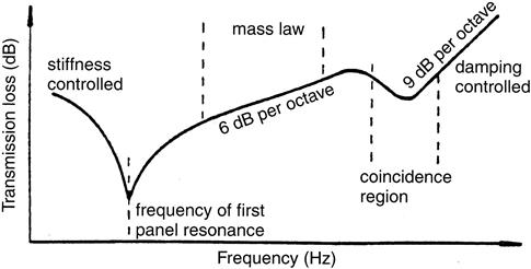
The propagation of audio-frequency waves through panels and walls is primarily due to the excitation of bending waves, which are a combination of shear and compressional waves. When a panel is of finite extent then a number of resonances are set up in the panel that are dependent on the bending stiffness of the panel. The frequency of the first panel resonance, f1, is given by
(6.8)
The second resonance occurs at the “coincidence” frequency, fc, when the projected wavelength of the incident sound coincides with the wavelength of the bending wave in the panel. The coincidence frequency is given by
(6.9)
The amount of sound transmitted by a panel is dependent on the surface weight, the damping of the panel, and the frequency of the sound. For a finite panel exposed to a random noise field, the acoustic behavior is specified mathematically as follows:
(6.10)
(6.10a)
(6.10b)
In most practical situations the lowest resonance frequency is below the audio range. Above this frequency a broad frequency range occurs in which the transmission loss is controlled by the surface weight and increases with frequency at the rate of 6 dB per octave. In the coincidence region the transmission loss is limited by the damping of the panel. Above the coincidence frequency the transmission loss increases by 9 dB per octave and is determined by the surface weight and the damping.
Clearly for a high value of sound reduction index over the majority of the audio-frequency range (the mass-controlled region) it is better to have a high surface weight, a low bending stiffness, and a high internal damping.
The acoustic performances of some materials have been predicted and are compared to measured values in Table 6–10. The data for 3-mm steel and 6-mm aluminum are shown in Figures 6–38 and 6–39. Each of the examples shown has the characteristic shape described above and the agreement between the measured and predicted values of transmission loss is good.
TABLE 6–10
Comparison of Predicted and Measured Sound Reduction Indices of Flat, Unlined Panels
| Sound Reduction Index, dB | |||||||||
| Material | Measured or Predicted | 63 | 125 | 250 | 500 | 1000 | 2000 | 4000 | 8000 |
| 3-mm steel | Predicted | 16 | 22 | 28 | 34 | 40 | 43 | 35 | 44 |
| Measured | 16 | 21 | 27 | 33 | 38 | 39 | 33 | – | |
| 6-mm steel | Predicted | 22 | 28 | 34 | 40 | 43 | 35 | 44 | 53 |
| Measured | 22 | 27 | 35 | 39 | 44 | 37 | 42 | – | |
| 6-mm aluminum | Predicted | 13 | 19 | 25 | 31 | 34 | 28 | 35 | 44 |
| Measured | 13 | 19 | 25 | 30 | 36 | 30 | 32 | – | |
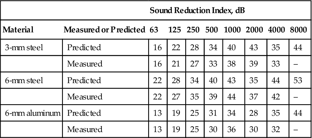
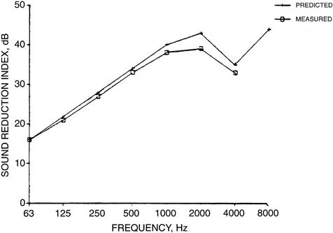
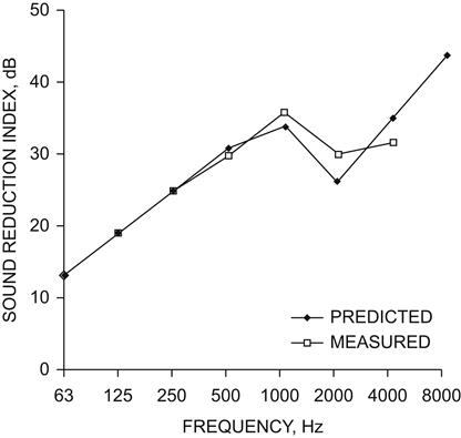
Sound Transmission through Unlined Corrugated Panels
In corrugated panels the characteristics of the panel are not the same in all directions. The moment of inertia across the corrugations differs from that parallel to the corrugations; thus the bending stiffness varies with direction. This affects both the first panel resonance and the coincidence frequency so that the sound transmission characteristics for these panels differ from flat panels with the same thickness. The first panel resonance is now given by
(6.11)
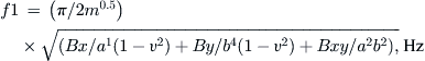 (6.11)
where Bx and By are the bending stiffnesses in the two principal planes of the panel and Bxy accounts for the torsional rigidity of the plate.
For real panels, measuring several meters in length and height, the frequency of this first resonance may still be in the subaudio range but can be several octaves higher than the first resonance of a flat panel of the same dimensions.
Since the coincidence frequency is determined by the bending stiffness, the presence of two bending stiffnesses gives rise to two critical frequencies, fcx and fcy, where
If the ratio of the bending stiffnesses, Bx and By, is less than 1.4, then the effects on the transmission loss of the panel will be small, but in typical panels the ratio of the bending stiffnesses is usually much greater than 1.4. This gives rise to a plateau in the transmission loss curve, which is illustrated in Figure 6–40. The plateau may extend over several decades for common corrugated or ribbed panels.
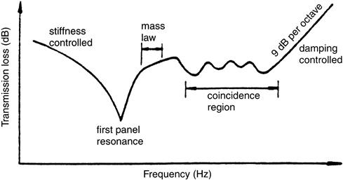
The sound transmission through orthotropic (corrugated) panels has been investigated by Heckl, who derived the following relationships for the diffuse field sound transmission:
(6.12)
(6.13)
where fcx and fcy are the two coincidence frequencies and where fcx is the lower of the two values.
The performances of two designs of corrugated panels have been predicted for panels made of 2.5-mm-thick steel with the designs shown in Figure 6–41. The predicted transmission losses are given in Table 6–11 and Figure 6–42.
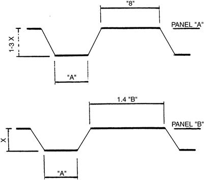
TABLE 6–11
Comparison of Predicted Sound Reduction Indices of Two Unlined Corrugated Panels
| Sound Reduction Index, dB | ||||||||
| 63 | 125 | 250 | 500 | 1000 | 2000 | 4000 | 8000 | |
| Panel A | 15 | 18 | 21 | 24 | 28 | 32 | 37 | 38 |
| Panel B | 15 | 21 | 24 | 25 | 29 | 33 | 37 | 38 |
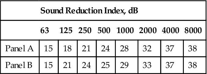
(Source: AFI Ltd.)
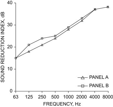
The predicted panel bending stiffnesses and resonant frequencies for the two panels are tabulated in Table 6–12 for a simply supported panel 4 m wide by 2.5 m high. The values for a flat panel of the same overall dimensions have also been included. The bending stiffness of panel B, in the direction parallel to the corrugations, is slightly less than that for panel A. This causes a shift in the lower critical frequency of about half an octave, which gives rise to a slightly higher transmission loss at lower frequencies.
TABLE 6–12
Predicted Parameters for Three Panels (Panels Made of Steel Measuring 4 m by 2.5 m by 2.5 mm Thick)
| Bending Stiffness, N⋅m | First Panel Resonance, Hz | Coincidence Frequency, Hz | |
| Panel A (corrugated) | trun -1240,000:241 | 30 | 163: 5115 |
| Panel B (corrugated) | 90,000:263 | 18 | 264: 4897 |
| Flat panel | 296 | 2.9 | 4825 |
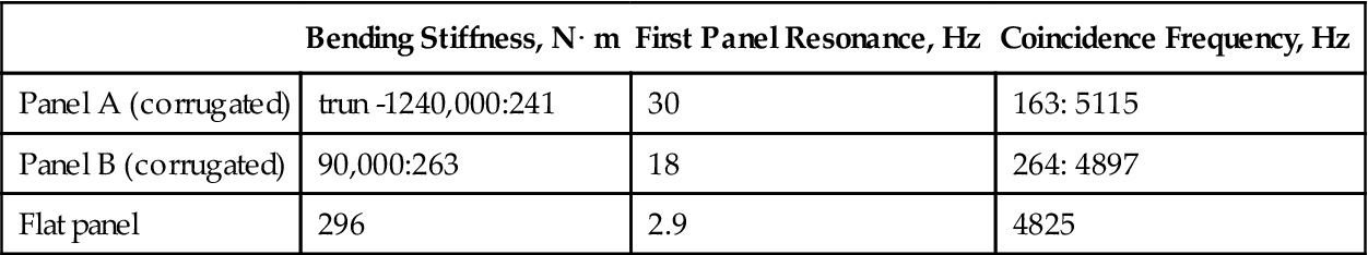
(Source: AFI Ltd.)
Transmission loss measurements have been carried out on a partition with the design of panel A. The test was carried out in accordance with the standard ISO 140 (1978). Table 6–13 and Figure 6–43 compare the predicted and measured performances. Both sets of curves show a plateau effect, which is more evident in the measured values. The predicted and measured values are within 4 dB of each other up to 4 kHz, above which the curves differ by about 7 dB. Although the agreement is not as close as for flat panels, it is encouraging. Of more interest is the comparison between the transmission losses of unlined, flat, and corrugated panels with the same thickness. Figure 6–44 and Table 6–14 show that the corrugated panel is substantially less effective in reducing sound transmission in the mid-frequencies compared to the flat panel equivalent.
TABLE 6–13
Predicted and Measured Sound Reduction Indices for Panel A
| Sound Reduction Index, dB | ||||||||
| 63 | 125 | 250 | 500 | 1000 | 2000 | 4000 | 8000 | |
| Predicted | 15 | 18 | 21 | 24 | 28 | 32 | 37 | 38 |
| Measured | 20 | 23 | 25 | 23 | 23 | 28 | 29 | 29 |
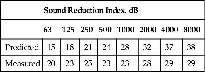
(Source: AFI Ltd.)
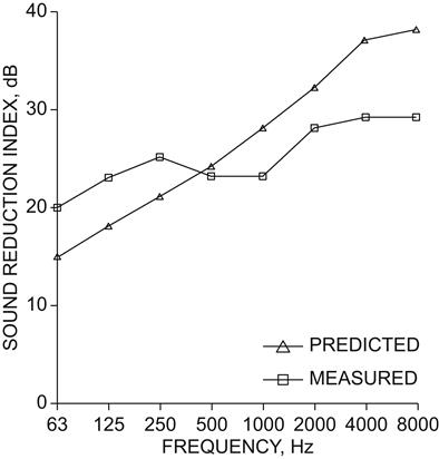
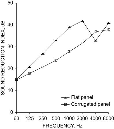
TABLE 6–14
Predicted Sound Reduction Indices for Flat Corrugated Panels (Panel Thickness of 2.5 mm)
| Sound Reduction Index, dB | ||||||||
| 63 | 125 | 250 | 500 | 1000 | 2000 | 4000 | 8000 | |
| Flat panel | 15 | 21 | 27 | 33 | 39 | 42 | 33 | 41 |
| Corrugated panel | 15 | 18 | 21 | 24 | 28 | 32 | 37 | 38 |
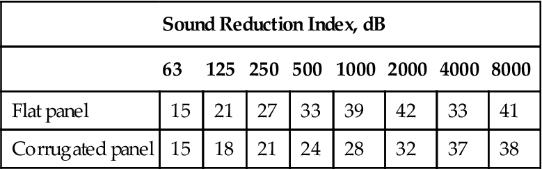
(Source: AFI Ltd.)
Clearly, if noise control is a primary consideration then unlined corrugated panels are not recommended, unless other engineering considerations dictate their use. Corrugated panels offer a considerable increase in bending stiffness, compared to flat panels, which reduces the amount of additional stiffening that would be required for a flat panel. But the volume of material required to produce a corrugated panel is significantly greater than that for a flat panel. For the two corrugated panel designs considered above, panel A contains 23% more material than the flat panel, and panel B contains 13% more material. Depending on the structural requirements, the additional stiffening required for a flat panel may result in a material savings when a corrugated design is chosen, especially if the flat panel is much thicker to compensate for its inherent low bending stiffness.
Attenuation of Sound by Absorptive Linings
Sound-absorbent linings are frequently fitted in acoustic enclosures to reduce the buildup of reverberant noise inside the enclosure. Typical reductions in the reverberant noise level may be between 3 and 10 dB depending on the application. An additional benefit is the increase in transmission loss of the enclosure panel, which further reduces the noise level outside the enclosure.
The increase in panel transmission loss arises because of several mechanisms. First, if the absorbent lining is sufficiently heavy and the panel is relatively thin, then the added layer may give sufficient additional weight to affect the “mass-law” performance and increase the damping of the panel. At high frequencies the absorbent may be relatively thick in comparison to the wavelength of the sound. The high-frequency sound may be attenuated not only because of the impedance mismatch between the air and the absorbent, but as the sound wave passes through the added layer a significant amount of acoustic energy is converted into heat by viscous losses in the interstices. In practice, the amount of heat generated is minute.
It is possible to distinguish between three frequency regions in which different attenuating mechanisms are predominant. For convenience these are described as regions A, C, and B, where A is the low-frequency region, C is the high-frequency region, and B is the transition region. The boundaries between these three regions are defined by the physical characteristics of the absorptive material in terms of the flow resistivity and the material thickness.
The flow resistivity of fibrous absorptive materials is dependent upon the bulk density and fiber diameter by the approximate relationship.
The frequency limits of the three regions, A, B, and C, are defined by
Region A: 101 < λm
Region B: 101 > λm, αl < 9 dB
Region C: αl > 9 dB
The values of λm, the wavelength of the sound inside the absorptive layer, and α, the attenuation constant for the material, can be measured or predicted for semirigid materials:
(6.14)
(6.15)
For an absorptive layer of known thickness and flow resistivity, the attenuation predicted from the equations given above is additive to that produced by the unlined panel.
The predicted and measured acoustic performances of two flat panels and one corrugated panel, each with an absorptive lining, are shown in Table 6–15 and Figures 6–45 to 6–47.
TABLE 6–15
Comparison of Predicted and Measured Sound Reduction Indices of Three Lined Panels
| Sound Reduction Index, dB | |||||||||
| Measured or Predicted | 63 | 125 | 250 | 500 | 1000 | 2000 | 4000 | 8000 | |
| Panel 1 (flat) | Predicted | 14 | 22 | 31 | 39 | 48 | 47 | 65 | 63 |
| Measured | 20 | 21 | 27 | 38 | 48 | 58 | 67 | 66 | |
| Panel 2 (flat) | Predicted | 20 | 30 | 40 | 46 | 52 | 60 | 63 | 79 |
| Measured | 31 | 34 | 35 | 44 | 54 | 63 | 62 | 68 | |
| Panel 3 (flat) | Predicted | 16 | 19 | 22 | 27 | 36 | 44 | 52 | 56 |
| (corrugated) | Measured | 22 | 24 | 28 | 32 | 38 | 48 | 52 | 52 |
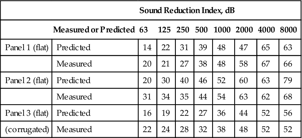
Panel 1: 1.6 mm flat steel lined with 100 mm thick glass fiber, 49 kg/m3 density.
Panel 2: 5 mm flat steel lined with 100 mm thick glass fiber, 48 kg/m3 density.
Panel 3: 2.5 mm corrugated steel lined with 50 mm thick mineral wool, 64 kg/m3 density.
(Source: AFI Ltd.)
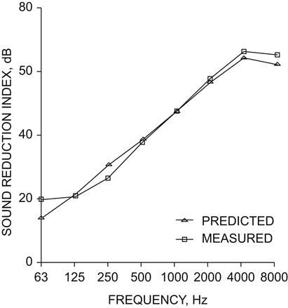
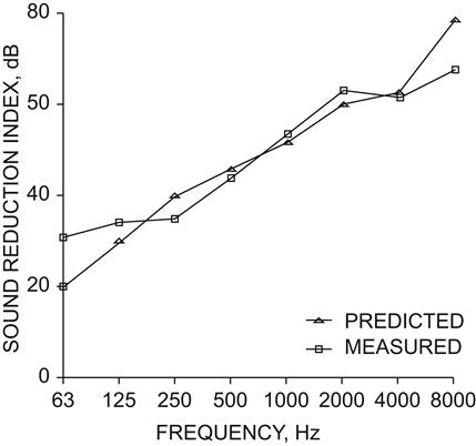
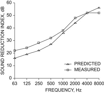
The predicted performances of the two flat panels are in good agreement with the measured performances over the majority of the frequency range. The largest discrepancies occur at 63 Hz and 8 kHz.
The agreement between the theoretical and measured performances of the corrugated panel is not as good as for the flat panel. The largest discrepancies occur at the lower frequencies with better agreement occurring at high frequencies. This follows the low-frequency trend shown in Figure 6–44 where the corrugated panel was unlined and the predicted performance was less than the measured performance by 5 dB. Nevertheless, the agreement is sufficiently close to support the theoretical model.
Experience Thus Far
It has been shown that the acoustic performance of lined and unlined panels can be predicted with reasonable accuracy for flat and corrugated panels. It has also been shown that, where noise control is important, unlined corrugated panels are not recommended unless other engineering considerations dictate their use, because corrugated panels are intrinsically less effective as sound insulators than flat panels of the same thickness.
A lining of sound absorptive material can substantially increase the sound reduction index of panels and the additional attenuation depends on the density, fiber diameter, and thickness of the lining. By careful selection of these parameters, the acoustic disadvantages of corrugated panels can be considerably reduced so that corrugated panels can be used confidently in situations where noise control is a primary requirement. The additional bending stiffness of corrugated panels permits a thinner outer skin to be employed and reduces the amount of additional bracing required to provide the structural integrity necessary in the demanding environment offshore. This reduction in overall weight compensates for the additional material used in forming the corrugations.
By careful design of the panel, a corrugation profile can be selected, which provides the most cost-effective solution when structural integrity, weight cost, ease of manufacture, and acoustic performance are considered. When expensive materials, such as stainless steel and aluminum, are employed, the reduction in cost by using a thinner-walled corrugated panel can be considerable.
A further consideration is the fire rating of lined corrugated panels. The normal requirement for bulkheads and decks offshore is the “A-60” class division. Corrugated panel designs of the type described here have been submitted to, and approved by, the appropriate authorities.
In some situations where a particularly high acoustic performance is called for, the corrugated design lends itself well to a multilayer construction employing an additional inner layer of heavy impervious material. Cheaper materials are used for the additional septum rather than for the outer skin. The acoustic attenuation of these multilayer designs is comparable to the performance of flat panels employing outer skins of twice the thickness of the corrugated outer skin. Figure 6–48 compares the measured performances of a traditional 5-mm-thick flat panel design with a 100-mm-thick absorptive lining and a multilayered panel based on a 2.5-mm-thick corrugated panel lined with a 50-mm absorptive layer.
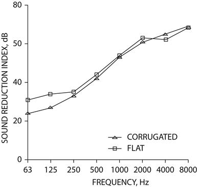
The nominal surface weights of the two designs are 50 kg/m2 and 40 kg/m2 for the flat and corrugated panels, respectively. Except at 63 and 125 Hz, the performance of the two panels is very similar.
In Summary
The acoustic performance of corrugated and flat steel panels can be predicted. The acoustic behavior of corrugated panels is very different from that of flat panels. This means that if corrugated panels are required, careful consideration must be given to the design, since unlined corrugated panels are unsuitable on their own for noise control applications.
However, the greater bending stiffness of corrugated panels offers many financial and structural advantages in the demanding environment that exists offshore, especially for gas turbines.
By lining the interior of a corrugated panel with a material whose physical parameters have been carefully chosen, the inherent acoustic weaknesses can be overcome. Thus a more cost-effective approach to gas turbine enclosure design can be adopted, which considers the structural integrity, weight, cost, ease of manufacture, and acoustic performance. The resultant designs employ less bracing and thinner outer skins to achieve the same acoustic performance as flat-walled constructions weighing typically 25% more than the equivalent corrugated design.