
Performance, Performance Testing, and Performance Optimization1
Abstract
Gas turbine performance, performance verification, and maintenance are irrevocably linked in an end user’s world. In summary, gas turbine performance verification (testing) is done at several levels. The testing of new GTs, done at the OEM’s facility, may be witnessed by end-user reps. Sometimes functional, no-load tests are conducted. Load testing is far more expensive than functional testing but critical in cases where the application or engine model is in some way different from previous applications. One small component change or instrument system change could change what was a successful gas turbine system without that change. OEMs may conduct tests to check a modified component. Frequently, they negotiate with an existing end user to check a new development in an existing plant application. Repair and overhaul is done by OEMs and independent shops. This chapter includes several case studies covering performance and performance verification.
Keywords
Performance theory; performance testing; performance optimization; performance verification; repair and overhaul
“Our doubts are traitors and make us lose the good we oft might win by fearing to attempt.”
—William Shakespeare
Gas turbine performance, performance verification, and maintenance are irrevocably linked in an end user’s world. In this book, however, maintenance is dealt with in Chapter 12.
In summary, gas turbine performance verification (testing) is done at several levels. The testing of new GTs, done at the OEM’s facility, may be witnessed by end-user reps. If the OEM is supplying a GT package (for instance, the GT and another OEM’s associated equipment), the OEM may elect to do a different battery of tests. Sometimes functional, no-load tests are conducted. Load testing is far more expensive than functional testing but critical in cases where the application or engine model is in some way different from previous applications. One small component change or instrument system change could change what was a successful gas turbine system without that change.
In the manufacture of GTs, OEMs sometimes have licensee manufacturers for the GT itself or portions of the system. GE is one such manufacturer.
All OEMs have vendors who supply accessory packages of some kind to the GT system, for instance a compressor washing skid. In testing new GTs or GT systems, these external vendor systems may be “slaved.” This means the OEM’s test facility has a duplicate model of the same system that is used for their tests. After the test, the slave is removed and kept for the next test and the gas turbine package gets a new unit or system design duplicate of the item that was slaved. In some cases, the actual units supplied with the package may be on the skid and tested along with the rest of the gas turbine system.
OEMs may conduct tests to check a modified component. Frequently, they negotiate with an existing end user to check a new development in an existing plant application.
Repair and overhaul is done by OEMs and independent shops. OEMs and independents may have licensees who are permitted to work on their machinery or specific components or processes (for instance, heat treatment, EDM, and powder metallurgy) within specific turbine models.
When an existing system needs to be optimized, the best designer for the project may or may not be the OEM: this is the end user’s choice. An independent (non-OEM) firm may work with the OEM’s knowledge and assistance or not. Some former-OEM-employee founded companies can be useful to end users for reverse engineering (for instance, making a component from studying an existing component), retrofit (adding to the existing GT package), or reengineering (redesigning a component or system that doesn’t work) projects.
In an operational context, a GT system needs to be monitored for performance degradation. Frequently, the cause of performance degradation is flow blockage, either in the compressor (potentially due to fouling) or turbine (potentially due to component deterioration or failure).
Generally, unless components are damaged permanently, compressor performance can be recovered with washing the compressor. The washing can be online or offline, at operating speed or reduced speed, and done with water plus additives, cleaning fluid, rice husks, or other mildly abrasive solid material (which still will not damage metal airfoils).
Certain values of CDP (compressor differential pressure) and compressor mass flow rate (this may be computed with other readings including compressor outlet temperature) have set points that trigger a wash when required. The wash may be done “online” at anywhere from slow roll to operational speed. It may be done “offline” with the rotor being slow rolled. It may also be done with a “crank soak,” where the wash fluid in inserted and left to sit while it dissolves and removes the contaminants.
The diagnostics required to pinpoint turbine module problems require similar readings for flow, pressure, and temperature. The preceding paragraphs in this section describe what is termed a performance analysis (PA) system.
The best PA systems work by comparing real live data (diagnostic) versus design (intended or “predicted”) data. The reference points for such a system must be worked out for each turbine model type, a process that requires cooperation with the OEM (to the extent that it requires the design curves and design data for a specific model). In certain customized projects (such as one where old GE2 Frame 5s with retrofitted steam injection took turbine model discs out of premature crack mode and provided augmented power), the original design data may be hard to find. In this case, reverse engineering may be required.
PA is extremely valuable, with a quick ROI (return on investment), especially in countries where fuel is expensive, fuel conservation is valued, or emissions taxed. Even if one is in a “fuel is cheap” location, PA can provide early warning signs of turbine component malfunction or failure. A couple of examples of a PA system “at work” follow.
Detecting turbine component deterioration and avoiding disastrous failure long before the turbine was scheduled for major overhaul. The turbine would have failed if regular TBOs had been observed.2
Gaining 0.1% efficiency on the turbine module of a GE Frame 7. For the reference US gas prices, that efficiency loss represented about $800,000 per GT annually.2
In terms of regular maintenance (covered in Chapter 12, Maintenance, Repair, and Overhaul), each GT has its own maintenance schedule, which is detailed in the O&M manuals. In general, there is:
Ongoing and regular maintenance (which may include oil sampling, borescope inspection, and items that do not require appreciable teardown).
Hot section inspections (HSIs) that check out the hot section (combustor including fuel nozzles and turbine).
Regular inspections (the extracts of a paper in this section give typical examples of those intervals).
Shutdown/turnaround/postfailure audits and other non-regular inspections occur when some major overhaul or parts replacement is made necessary by a machinery failure or major modification) or plant shutdown for other reasons, such as an expansion.
Note that maintenance is differentiated from GT engine condition monitoring systems (ECMS), which may include:
ECMS, as we saw in the previous chapter, is a vast topic. While VA and to some extent PA were covered in the previous chapter, some aspects of LCA and PA are covered in this one.
Performance
A good starting point for considering theoretical performance and performance optimization is theoretical cycle diagrams (see Chapter 3, Gas Turbine Configurations and Heat Cycles). From that chapter, it was noted that:
1. Intercooling during compression,
2. Adding (exhaust waste) heat to the compressed gases prior to combustion (recuperation),
all add to the efficiency of the gas turbine cycle.
Further cycle efficiency improvements can be made by:
1. Cooling inlet air (cooler air is denser and provides more power per unit volume of inlet air).
2. Other waste heat recovery and cogeneration, such as waste heat being used in a HRSG (heat recovery steam generator) to run a steam turbine with the gas turbine (a combined cycle).
3. A variation in principle of an aircraft engine afterburner in land-based applications injects a fuel source downstream of the gas turbine exhaust and ignites the exhaust air/supplementary fuel mix for additional power.
In addition to these basic cycle adaptations and variations on a theme thereof, gas turbine users now also use inlet air fogging (for cooling inlet air) and steam and/or water injection for power augmentation. The latter means, sometimes used for NOx reduction or cooling (for instance, to take turbine discs out of heat damage range, such as a premature hot section component crack zone), can result in 20–25% additional power developed.
There are a myriad of other performance retention and optimization technologies. They include the science of performance recovery with (online or otherwise) compressor washing or cleaning with liquid or solid cleaning media.
Performance optimization can also be described as improved TBOs and increased MTBFs (mean time between failures). For optimization of TBOs, LCA is a valuable tool. The algorithms used by OEMs to calculate a cycle of life used per engine type vary among OEMs and different models for the same OEM. However, all generally result in extended service lives for major hot section components (over what used to be stated lives in hours of operation that had a large safety factor applied).
The author’s course notes on a basic course on PA and LCA are included here. These notes do not give away any proprietary algorithms but do indicate how they may be derived, in principle, with specific parameters. Also covered are the applications of some of the hardware/software packages used to conduct LCA and potential for these packages to be retrofitted.
Note also that several performance-related basic accessory system descriptions were covered in Chapter 8, Accessory Systems. These include:
1. Thrust distribution and specific features that can direct thrust for different (vertical/short takeoff and landing systems, afterburners, and so forth) applications
Before the case studies for this chapter, the following theory will be useful. The source is Rolls Royce’s The Jet Engine; however, land-based users are advised again that all aircraft engine technology is directly applicable to all gas turbines at some point. This is true whether the aircraft engines are in helicopters (power stated in shaft horsepower) or jet service (power stated in pounds of thrust).
Performance Theory Summary3
The performance requirements of an engine are obviously dictated to a large extent by the type of operation for which the engine is designed. The power of the turbo-jet engine is measured in thrust, produced at the propelling nozzle or nozzles, and that of the turbo-propeller engine is measured in shaft horse-power (s.h.p.) produced at the propeller shaft. However, both types are in the main assessed on the amount of thrust or s.h.p. they develop for a given weight, fuel consumption and frontal area.
Since the thrust or s.h.p. developed is dependent on the mass of air entering the engine and the acceleration imparted to it during the engine cycle, it is obviously influenced, as subsequently described, by such variables as the forward speed of the aircraft, altitude, and climatic conditions. These variables influence the efficiency of the air intake, the compressor, the turbine, and the jet pipe; consequently, the gas energy available for the production of thrust or s.h.p. also varies.
In the interest of fuel economy and aircraft range, the ratio of fuel consumption to thrust or s.h.p. should be as low as possible. This ratio, known as the specific fuel consumption (s.f.c.), is expressed in pounds of fuel per hour per pound of net thrust or s.h.p. and is determined by the thermal and propulsive efficiency of the engine. In recent years considerable progress has been made in reducing s.f.c. and weight. These factors are further explained later.
Whereas the thermal efficiency is often referred to as the internal efficiency of the engine, the propulsive efficiency is referred to as the external efficiency. This latter efficiency, described later, explains why the pure jet engine is less efficient than the turbo-propeller engine at lower aircraft speeds leading to development of the bypass principle and, more recently, the propfan designs.
The thermal and the propulsive efficiency also influence, to a large extent, the size of the compressor and turbine, thus determining the weight and diameter of the engine for a given output.
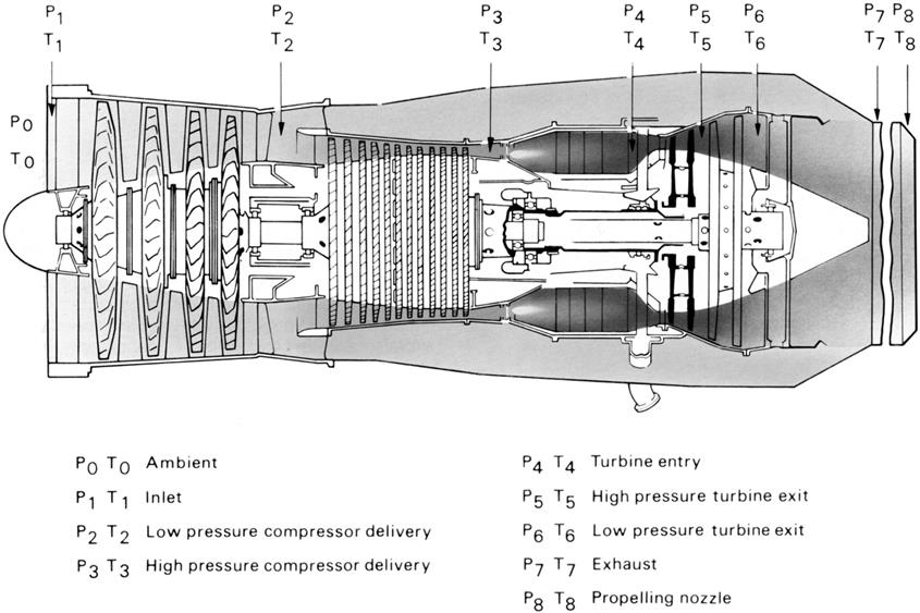
These and other factors are presented in curves and graphs, calculated from the basic gas laws, and are proved in practice by bench and flight testing, or by simulating flight conditions in a high altitude test cell. To make these calculations, specific symbols are used to denote the pressures and temperatures at various locations through the engine; for instance, using the symbols shown in Figure 10–1 the overall compressor pressure ratio is P3/P1. These symbols vary slightly for different types of engine; for instance, with high bypass ratio engines, and also when afterburning is incorporated, additional symbols are used.
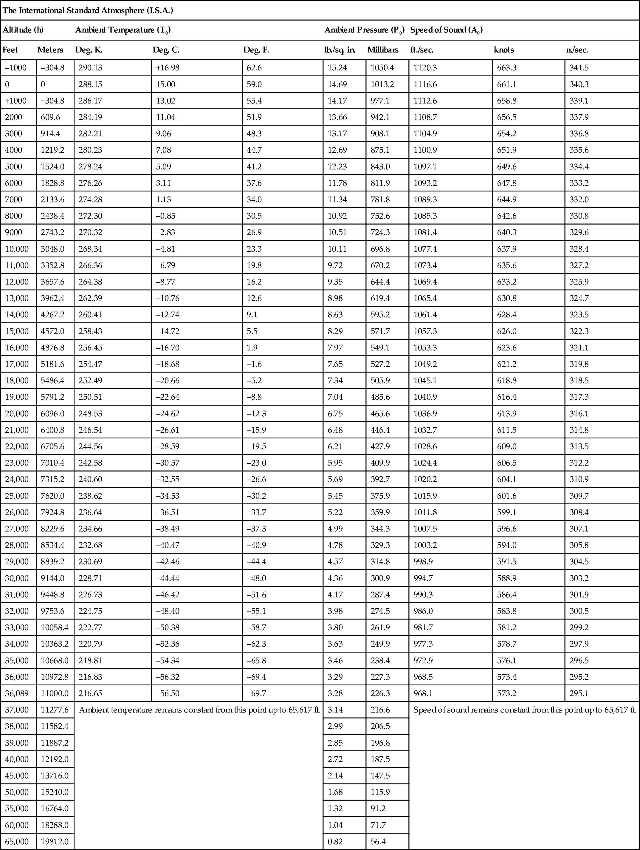
To enable the performance of similar engines to be compared, it is necessary to standardize in some conventional form the variations of air temperature and pressure that occur with altitude and climatic conditions. There are in use several different definitions of standard atmospheres, the one in most common use being the International Standard Atmosphere (I.S.A.). This is based on a temperature lapse rate of approximately 1.98K per 1000 ft., resulting in a fall from 288.15K. (15°C) at sea level to 216.65K (–56.5°C) at 36,089 ft. (the tropopause). Above this altitude the temperature is constant up to 65,617 ft. The I.S.A. temperature is constant up to 65,617 ft. The I.S.A. standard pressure at sea level is 14.69 pounds per square inch falling to 3.28 pounds per square inch at the tropopause (refer to I.S.A. Table 10–1, at the end of this section).
TABLE 10–1
The International Standard Atmosphere (I.S.A.)
| The International Standard Atmosphere (I.S.A.) | |||||||||
| Altitude (h) | Ambient Temperature (T0) | Ambient Pressure (P0) | Speed of Sound (A0) | ||||||
| Feet | Meters | Deg. K. | Deg. C. | Deg. F. | lb./sq. in. | Millibars | ft./sec. | knots | n./sec. |
| –1000 | –304.8 | 290.13 | +16.98 | 62.6 | 15.24 | 1050.4 | 1120.3 | 663.3 | 341.5 |
| 0 | 0 | 288.15 | 15.00 | 59.0 | 14.69 | 1013.2 | 1116.6 | 661.1 | 340.3 |
| +1000 | +304.8 | 286.17 | 13.02 | 55.4 | 14.17 | 977.1 | 1112.6 | 658.8 | 339.1 |
| 2000 | 609.6 | 284.19 | 11.04 | 51.9 | 13.66 | 942.1 | 1108.7 | 656.5 | 337.9 |
| 3000 | 914.4 | 282.21 | 9.06 | 48.3 | 13.17 | 908.1 | 1104.9 | 654.2 | 336.8 |
| 4000 | 1219.2 | 280.23 | 7.08 | 44.7 | 12.69 | 875.1 | 1100.9 | 651.9 | 335.6 |
| 5000 | 1524.0 | 278.24 | 5.09 | 41.2 | 12.23 | 843.0 | 1097.1 | 649.6 | 334.4 |
| 6000 | 1828.8 | 276.26 | 3.11 | 37.6 | 11.78 | 811.9 | 1093.2 | 647.8 | 333.2 |
| 7000 | 2133.6 | 274.28 | 1.13 | 34.0 | 11.34 | 781.8 | 1089.3 | 644.9 | 332.0 |
| 8000 | 2438.4 | 272.30 | –0.85 | 30.5 | 10.92 | 752.6 | 1085.3 | 642.6 | 330.8 |
| 9000 | 2743.2 | 270.32 | –2.83 | 26.9 | 10.51 | 724.3 | 1081.4 | 640.3 | 329.6 |
| 10,000 | 3048.0 | 268.34 | –4.81 | 23.3 | 10.11 | 696.8 | 1077.4 | 637.9 | 328.4 |
| 11,000 | 3352.8 | 266.36 | –6.79 | 19.8 | 9.72 | 670.2 | 1073.4 | 635.6 | 327.2 |
| 12,000 | 3657.6 | 264.38 | –8.77 | 16.2 | 9.35 | 644.4 | 1069.4 | 633.2 | 325.9 |
| 13,000 | 3962.4 | 262.39 | –10.76 | 12.6 | 8.98 | 619.4 | 1065.4 | 630.8 | 324.7 |
| 14,000 | 4267.2 | 260.41 | –12.74 | 9.1 | 8.63 | 595.2 | 1061.4 | 628.4 | 323.5 |
| 15,000 | 4572.0 | 258.43 | –14.72 | 5.5 | 8.29 | 571.7 | 1057.3 | 626.0 | 322.3 |
| 16,000 | 4876.8 | 256.45 | –16.70 | 1.9 | 7.97 | 549.1 | 1053.3 | 623.6 | 321.1 |
| 17,000 | 5181.6 | 254.47 | –18.68 | –1.6 | 7.65 | 527.2 | 1049.2 | 621.2 | 319.8 |
| 18,000 | 5486.4 | 252.49 | –20.66 | –5.2 | 7.34 | 505.9 | 1045.1 | 618.8 | 318.5 |
| 19,000 | 5791.2 | 250.51 | –22.64 | –8.8 | 7.04 | 485.6 | 1040.9 | 616.4 | 317.3 |
| 20,000 | 6096.0 | 248.53 | –24.62 | –12.3 | 6.75 | 465.6 | 1036.9 | 613.9 | 316.1 |
| 21,000 | 6400.8 | 246.54 | –26.61 | –15.9 | 6.48 | 446.4 | 1032.7 | 611.5 | 314.8 |
| 22,000 | 6705.6 | 244.56 | –28.59 | –19.5 | 6.21 | 427.9 | 1028.6 | 609.0 | 313.5 |
| 23,000 | 7010.4 | 242.58 | –30.57 | –23.0 | 5.95 | 409.9 | 1024.4 | 606.5 | 312.2 |
| 24,000 | 7315.2 | 240.60 | –32.55 | –26.6 | 5.69 | 392.7 | 1020.2 | 604.1 | 310.9 |
| 25,000 | 7620.0 | 238.62 | –34.53 | –30.2 | 5.45 | 375.9 | 1015.9 | 601.6 | 309.7 |
| 26,000 | 7924.8 | 236.64 | –36.51 | –33.7 | 5.22 | 359.9 | 1011.8 | 599.1 | 308.4 |
| 27,000 | 8229.6 | 234.66 | –38.49 | –37.3 | 4.99 | 344.3 | 1007.5 | 596.6 | 307.1 |
| 28,000 | 8534.4 | 232.68 | –40.47 | –40.9 | 4.78 | 329.3 | 1003.2 | 594.0 | 305.8 |
| 29,000 | 8839.2 | 230.69 | –42.46 | –44.4 | 4.57 | 314.8 | 998.9 | 591.5 | 304.5 |
| 30,000 | 9144.0 | 228.71 | –44.44 | –48.0 | 4.36 | 300.9 | 994.7 | 588.9 | 303.2 |
| 31,000 | 9448.8 | 226.73 | –46.42 | –51.6 | 4.17 | 287.4 | 990.3 | 586.4 | 301.9 |
| 32,000 | 9753.6 | 224.75 | –48.40 | –55.1 | 3.98 | 274.5 | 986.0 | 583.8 | 300.5 |
| 33,000 | 10058.4 | 222.77 | –50.38 | –58.7 | 3.80 | 261.9 | 981.7 | 581.2 | 299.2 |
| 34,000 | 10363.2 | 220.79 | –52.36 | –62.3 | 3.63 | 249.9 | 977.3 | 578.7 | 297.9 |
| 35,000 | 10668.0 | 218.81 | –54.34 | –65.8 | 3.46 | 238.4 | 972.9 | 576.1 | 296.5 |
| 36,000 | 10972.8 | 216.83 | –56.32 | –69.4 | 3.29 | 227.3 | 968.5 | 573.4 | 295.2 |
| 36,089 | 11000.0 | 216.65 | –56.50 | –69.7 | 3.28 | 226.3 | 968.1 | 573.2 | 295.1 |
| 37,000 | 11277.6 | Ambient temperature remains constant from this point up to 65,617 ft. | 3.14 | 216.6 | Speed of sound remains constant from this point up to 65,617 ft. | ||||
| 38,000 | 11582.4 | 2.99 | 206.5 | ||||||
| 39,000 | 11887.2 | 2.85 | 196.8 | ||||||
| 40,000 | 12192.0 | 2.72 | 187.5 | ||||||
| 45,000 | 13716.0 | 2.14 | 147.5 | ||||||
| 50,000 | 15240.0 | 1.68 | 115.9 | ||||||
| 55,000 | 16764.0 | 1.32 | 91.2 | ||||||
| 60,000 | 18288.0 | 1.04 | 71.7 | ||||||
| 65,000 | 19812.0 | 0.82 | 56.4 | ||||||
(Source: Rolls Royce)
Engine Thrust in Test
The thrust of the turbo-jet engine on the test bench differs somewhat from that during flight. Modern test facilities are available to simulate atmospheric conditions at high altitudes thus providing a means of assessing some of the performance capability of a turbo-jet engine in flight without the engine ever leaving the ground. This is important as the changes in ambient temperature and pressure encountered at high altitudes considerably influence the thrust of the engine.
Considering the formula derived later for engines operating under “choked” nozzle conditions,
it can be seen that the thrust can be further affected by a change in the mass flow rate of air through the engine and by a change in jet velocity. An increase in mass airflow may be obtained by using water injection and increases in jet velocity by using afterburning.
As previously mentioned, changes in ambient pressure and temperature considerably influence the thrust of the engine. This is because of the way they affect the air density and hence the mass of air entering the engine for a given engine rotational speed. To enable the performance of similar engines to be compared when operating under different climatic conditions, or at different altitudes, correction factors must be applied to the calculations to return the observed values to those that would be found under I.S.A. conditions. For example, the thrust correction for a turbo-jet engine is:
The observed performance of the turbo-propeller engine is also corrected to I.S.A. conditions, but due to the rating being in s.h.p. and not in pounds of thrust the factors are different. For example, the correction for s.h.p. is:
P0 = atmospheric pressure (in. Hg.) (observed)
T0 = atmospheric temperature in °C (observed)
30 = I.S.A. standard sea level pressure (in. Hg.)
In practice there is always a certain amount of jet thrust in the total output of the turbo-propeller engine and this must be added to the s.h.p. The correction for jet thrust is the same as that stated earlier.
To distinguish between these two aspects of the power output, it is usual to refer to them as s.h.p. and thrust horsepower (t.h.p.). The total equivalent horsepower is denoted by t.e.h.p. (sometimes e.h.p.) and is the s.h.p. plus the s.h.p. equivalent to the net jet thrust. For estimation purposes it is taken that, under sea-level static conditions, one s.h.p. is equivalent to approximately 2.6 lb. of jet thrust. Therefore:
The ratio of jet thrust to shaft power is influenced by many factors. For instance, the higher the aircraft operating speed the larger may be the required proportion of total output in the form of jet thrust. Alternatively, an extra turbine stage may be required if more than a certain proportion of the total power is to be provided at the shaft. In general, turbo-propeller aircraft provide one pound of thrust for every 3.5 h.p. to 5 h.p.
Comparison between Thrust and Horse-Power
Because the turbo-jet engine is rated in thrust and the turbo-propeller engine in s.h.p., no direct comparison between the two can be made without a power conversion factor. However, since the turbo-propeller engine receives its thrust mainly from the propeller, a comparison can be made by converting the horse-power developed by the engine to thrust or the thrust developed by the turbo-jet engine to t.h.p.; that is, by converting work to force or force to work. For this purpose, it is necessary to take into account the speed of the aircraft.
The t.h.p. is expressed as FV/(550 ft. per sec.) where
Since 1 horsepower is equal to 550 ft.lb. per sec. and 550 ft. per sec. is equivalent to 375 miles per hour, it can be seen from the above formula that 1 lb. of thrust equals 1 t.h.p. at 375 m.p.h. It is also common to quote the speed in knots (nautical miles per hour); one knot is equal to 1.1515 m.p.h. or 1 pound of thrust is equal to one t.h.p. at 325 knots.
Thus if a turbo-jet engine produces 5000 lb. of net thrust at an aircraft speed of 600 m.p.h. the t.h.p would be
However, if the same thrust was being produced by a turbo-propeller engine with a propeller efficiency of 55% at the same flight speed of 600 m.p.h., then the t.h.p. would be
Thus at 600 m.p.h. 1 lb. of thrust is the equivalent of about 3 t.h.p.
Engine Thrust in Flight
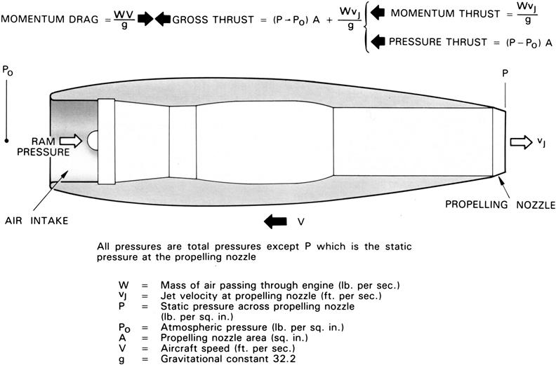
Since reference will be made to gross thrust, momentum drag, and net thrust, it will be helpful to define these terms:
• Gross or total thrust is the product of the mass of air passing through the engine and the jet velocity at the propelling nozzle, expressed as:
• The momentum drag is the drag due to the momentum of the air passing into the engine relative to the aircraft velocity is expressed as WV/g where
V = Velocity of aircraft in feet per sec.
g = Gravitational constant 32.2 ft. per sec.
• The net thrust or resultant force acting on the aircraft in flight is the difference between the gross thrust and the momentum drag.
From the definitions and formulae just stated; under flight conditions, the net thrust of the engine, simplifying can be expressed as:
Figure 10–2 provides a diagrammatic explanation.
Effect of Forward Speed
Since reference will be made to “ram ratio” and Mach number, these terms are defined as follows:
• Ram ratio is the ratio of the total air pressure at the engine compressor entry to the static air pressure at the air intake entry.
• Mach number is an additional means of measuring speed and is defined as the ratio of the speed of a body to the local speed of sound. Mach 1.0 therefore represents a speed equal to the local speed of sound.
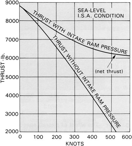
From the thrust equation, it is apparent that if the jet velocity remains constant, independent of aircraft speed, then as the aircraft speed increases the thrust would decrease in direct proportion. However, due to the “ram ratio” effect from the aircraft forward speed, extra air is taken into the engine so that the mass airflow and also the jet velocity increase with aircraft speed. The effect of this tends to offset the extra intake momentum drag due to the forward speed so that the resultant loss of net thrust is partially recovered as the aircraft speed increases. A typical curve illustrating this point is shown in Figure 10–3. Obviously, the “ram ratio” effect, or the return obtained in terms of pressure rise at entry to the compressor in exchange for the unavoidable intake drag, is of considerable importance to the turbo-jet engine, especially at high speeds. Above speeds of Mach 1.0, as a result of the formation of shock waves at the air intake, this rate of pressure rise will rapidly decrease unless a suitably designed air intake is provided; an efficient air intake is necessary to obtain maximum benefit from the ram ratio effect.
As aircraft speeds increase into the supersonic region, the ram air temperature rises rapidly consistent with the basic gas laws. This temperature rise affects the compressor delivery air temperature proportionately and, in consequence, to maintain the required thrust, the engine must be subjected to higher turbine entry temperatures. Since the maximum permissible turbine entry temperature is determined by the temperature limitations of the turbine assembly, the choice of turbine materials and the design of blades and stators to permit cooling are very important.
With an increase in forward speed, the increased mass airflow due to the “ram ratio” effect must be matched by the fuel flow and the result is an increase in fuel consumption. Because the net thrust tends to decrease with forward speed the end result is an increase in specific fuel consumption (s.f.c.), as shown by the curves for a typical turbo-jet engine in Figure 10–4.
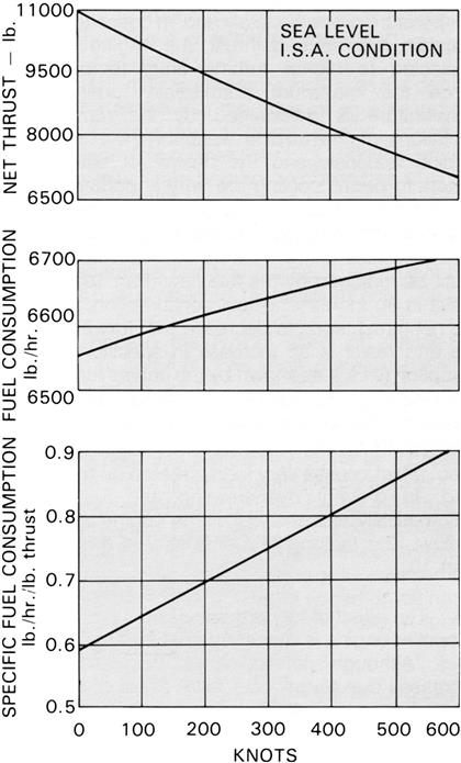
At high forward speeds at low altitudes the “ram ratio” effect causes very high stresses on the engine and, to prevent overstressing, the fuel flow is automatically reduced to limit the engine speed and airflow.
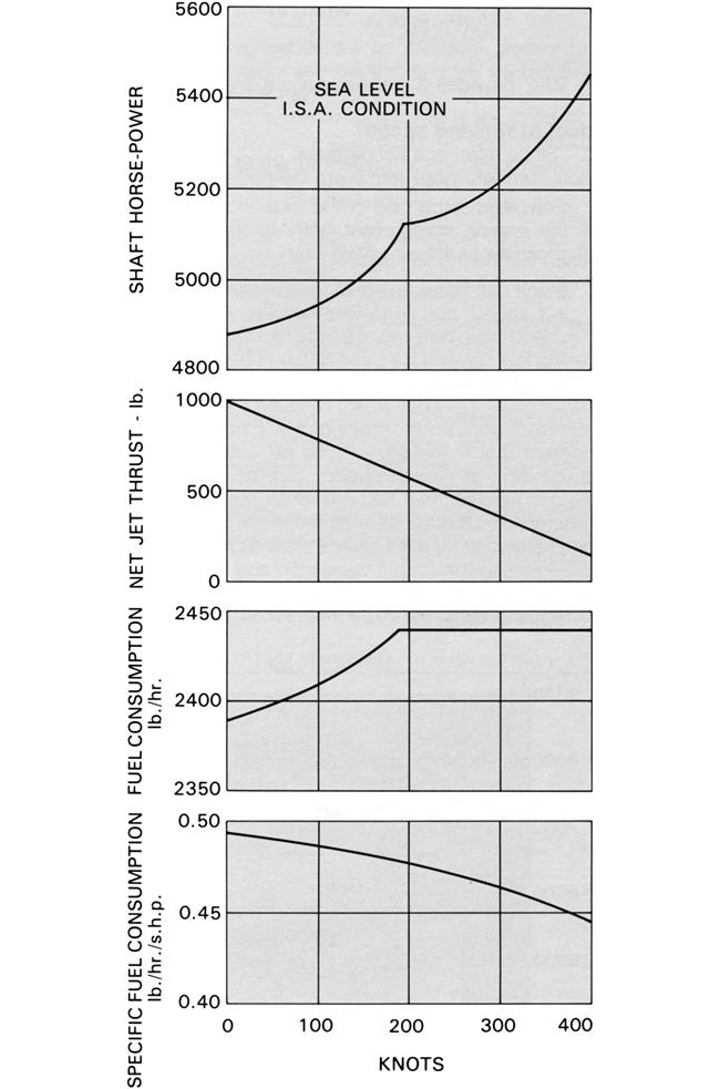
The effect of forward speed on a typical turbo-propeller engine is shown by the trend curves in Figure 10–5. Although net jet thrust decreases, s.h.p. increases due to the “ram ratio” effect of increased mass flow and matching fuel flow. Because it is standard practice to express the s.f.c. of a turbo-propeller engine relative to s.h.p., an improved s.f.c. is exhibited. However, this does not provide a true comparison with the curves shown in Figure 10–4, for a typical turbo-jet engine, as s.h.p. is absorbed by the propeller and converted into thrust and, irrespective of an increase in s.h.p., propeller efficiency and therefore net thrust deteriorates at high subsonic forward speeds. In consequence, the turbo-propeller engine s.f.c. relative to net thrust would, in general comparison with the turbo-jet engine, show an improvement at low forward speeds but a rapid deterioration at high speeds.
Effect of Afterburning on Engine Thrust
At takeoff conditions, the momentum drag of the airflow through the engine is negligible, so that the gross thrust can be considered to be equal to the net thrust. If afterburning is selected, an increase in takeoff thrust in the order of 30% is possible with the pure jet engine and considerably more with the bypass engine. This augmentation of basic thrust is of greater advantage for certain specific operating requirements.
Under flight conditions, however, this advantage is even greater, since the momentum drag is the same with or without afterburning and, due to the ram effect, better utilization is made of every pound of air flowing through the engine. The following example, illustrates why afterburning thrust improves under flight conditions.
Assuming an aircraft speed of 600 m.p.h. (880 ft. per sec.), then momentum drag is: 880/32.2 = 27.5 (approximately). This means that every pound of air per second flowing through the engine and accelerated up to the speed of the aircraft causes a drag of about 27.5 lb.
Suppose each pound of air passed through the engine gives a gross thrust of 77.5 lb. Then the net thrust given by the engine per lb. of air per second is 77.5 – 27.5 = 50 lb.
When afterburning is selected, assuming the 30% increase in static thrust given previously, the gross thrust will be 1.3 × 77.5 100.75 lb. Thus, under flight condition of 600 m.p.h., the net thrust per pound of air per second will be 100.75 – 27.5 = 73.25 lb. Therefore, the ratio of net thrust due to afterburning is 73.25/50 = 1.465. In other words a 30% increase in thrust under static conditions becomes a 46.5% increase in thrust at 600 m.p.h.
This larger increase in thrust is invaluable for obtaining higher speeds and higher altitude performances. The total and specific fuel consumptions are high, but not unduly so for such an increase in performance.
The limit to the obtainable thrust is determined by the afterburning temperature and the remaining usable oxygen in the exhaust gas stream. Because no previous combustion heating takes place in the duct of a bypass engine, these engines with their large residual oxygen surplus are particularly suited to afterburning and static thrust increases of up to 70% are obtainable. At high forward speeds several times this amount are achieved.
Effect of Altitude
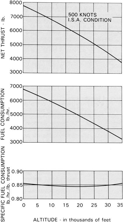
With increasing altitude the ambient air pressure and temperature are reduced. This affects the engine in two interrelated ways:
• The fall of pressure reduces the air density and hence the mass airflow into the engine for a given engine speed. This causes the thrust or s.h.p. to fall. The fuel control system adjusts the fuel pump output to match the reduced mass airflow, so maintaining a constant engine speed.
• The fall in air temperature increases the density of the air, so that the mass of air entering the compressor for a given engine speed is greater. This causes the mass airflow to reduce at a lower rate and so compensates to some extent for the loss of thrust due to the fall in atmospheric pressure. At altitudes above 36,089 feet and up to 65,617 feet, however, the temperature remains constant, and the thrust or s.h.p. is affected by pressure only.
Graphs showing the typical effect of altitude on thrust, s.h.p., and fuel consumption are illustrated in Figures 10–6 and 10–7.

Effect of Temperature
On a cold day the density of the air increases so that the mass of air entering the compressor for a given engine speed is greater, hence the thrust or s.h.p. is higher. The denser air does, however, increase the power required to drive the compressor or compressors: thus the engine will require more fuel to maintain the same engine speed or will run at a reduced engine speed if no increase in fuel is available.
On a hot day the density of the air decreases, thus reducing the mass of air entering the compressor and, consequently, the thrust of the engine for a given rpm. Because less power will be required to drive the compressor, the fuel control system reduces the fuel flow to maintain a constant engine rotational speed or turbine entry temperature, as appropriate; however, because of the decrease in air density, the thrust will be lower. At a temperature of 45°C, depending on the type of engine, a thrust loss of up to 20% may be experienced. This means that some sort of thrust augmentation, such as water injection, may be required.
The fuel control system controls the fuel flow so that the maximum fuel supply is held practically constant at low air temperature conditions, whereupon the engine speed falls but, because of the increased mass airflow as a result of the increase in air density, the thrust remains the same. For example, the combined acceleration and speed control fuel system schedules fuel flow to maintain a constant engine rpm, hence thrust increases as air temperature decreases until, at a predetermined compressor delivery pressure, the fuel flow is automatically controlled to maintain a constant compressor delivery pressure and, therefore, thrust. Figure 10–8 illustrates this for a twin-spool engine where the controlled engine rpm is high-pressure compressor speed and the compressor delivery pressure is expressed as P3. It will also be apparent from this graph that the low-pressure compressor speed is always less than its limiting maximum and that the difference in the two speeds is reduced by a decrease in ambient air temperature. To prevent the L.P. compressor overspeeding, fuel flow is also controlled by an L.P. governor which, in this case, takes a passive role.
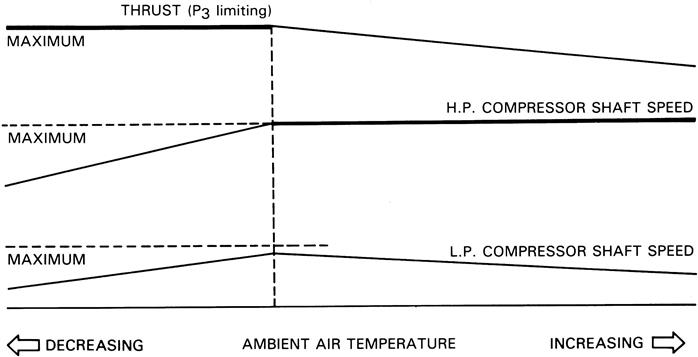
The pressure ratio control fuel system schedules fuel flow to maintain a constant engine pressure ratio and, therefore, thrust below a predetermined ambient air temperature. Above this temperature the fuel flow is automatically controlled to prevent turbine entry temperature limitations from being exceeded, thus resulting in reduced thrust and, overall, similar curve characteristics to those shown in Figure 10–8. In the instance of a triple-spool engine the pressure ratio is expressed as P4/P1, i.e., H.P. compressor delivery pressure/engine inlet pressure.
Propulsive Efficiency
Performance of the jet engine is not only concerned with the thrust produced, but also with the efficient conversion of the heat energy of the fuel into kinetic energy, as represented by the jet velocity, and the best use of this velocity to propel the aircraft forward, i.e., the efficiency of the propulsive system.
The efficiency of conversion of fuel energy to kinetic energy is termed thermal or internal efficiency and, like all heat engines, is controlled by the cycle pressure ratio and combustion temperature. Unfortunately, this temperature is limited by the thermal and mechanical stresses that can be tolerated by the turbine. The development of new materials and techniques to minimize these limitations is continually being pursued.
The efficiency of conversion of kinetic energy to propulsive work is termed the propulsive or external efficiency and this is affected by the amount of kinetic energy wasted by the propelling mechanism. Waste energy dissipated in the jet wake, which represents a loss, can be expressed as [W(vJ – V)2]/2g where (vJ – V) is the waste velocity. It is therefore apparent that at the aircraft lower speed range the pure jet stream wastes considerably more energy than a propeller system and consequently is less efficient over this range. However, this factor changes as aircraft speed increases, because although the jet stream continues to issue at a high velocity from the engine its velocity relative to the surrounding atmosphere is reduced and, in consequence, the waste energy loss is reduced.
Briefly, propulsive efficiency may be expressed as:
or simply
Work done is the net thrust multiplied by the aircraft speed. Therefore, progressing from the net thrust equation given earlier, the following equation is arrived at:
In the instance of an engine operating with a non-choked nozzle, the equation becomes:
Simplified to: 2V/(V + vj)
This latter equation can also be used for the choked nozzle condition by using VJ to represent the jet velocity when fully expanded to atmospheric pressure, thereby dispensing with the nozzle pressure term (P – P0)A.
Assuming an aircraft speed (V) of 375 m.p.h. and a jet velocity (vJ) of 1230 m.p.h., the efficiency of a turbo-jet is:
On the other hand, at an aircraft speed of 600 m.p.h. the efficiency is:
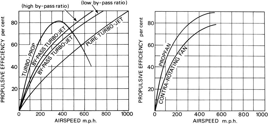
Propeller efficiency at these values of V is approximately 82 and 55%, respectively, and from reference to Figure 10–9 it can be seen that for aircraft designed to operate at sea level speeds below approximately 400 m.p.h. it is more effective to absorb the power developed in the jet engine by gearing it to a propeller instead of using it directly in the form of a pure jet stream. The disadvantage of the propeller at the higher aircraft speeds is its rapid fall off in efficiency, due to shock waves created around the propeller as the blade tip speed approaches Mach 1.0. Advanced propeller technology, however, has produced a multi-bladed, swept back design capable of turning with tip speeds in excess of Mach 1.0 without loss of propeller efficiency. By using this design of propeller in a contra-rotating configuration, thereby reducing swirl losses, a “prop-fan” engine, with very good propulsive efficiency capable of operating efficiently at aircraft speeds in excess of 500 m.p.h. at sea level, can be produced.
To obtain good propulsive efficiencies without the use of a complex propeller system, the bypass principle is used in various forms. With this principle, some part of the total output is provided by a jet stream other than that which passes through the engine cycle and this is energized by a fan or a varying number of L.P. compressor stages. This bypass air is used to lower the mean jet temperature and velocity either by exhausting through a separate propelling nozzle, or by mixing with the turbine stream to exhaust through a common nozzle.
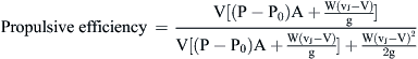
The propulsive efficiency equation for a high bypass ratio engine exhausting through separate nozzles is given below, where W1 and ![]() relate to the bypass function and W2 and
relate to the bypass function and W2 and ![]() to the engine main function.
to the engine main function.
Propulsive efficiency =
By calculation, substituting the following values, which will be typical of a high bypass ratio engine of triple-spool configuration, it will be observed that a propulsive efficiency of approximately 85% results.
Propulsive efficiency can be further improved by using the rear mounted contra-rotating fan configuration of the bypass principle. This gives very high bypass ratios in the order of 15:1, and reduced “drag” results due to the engine core being “washed” by the low velocity aircraft slipstream and not the relatively high velocity fan efflux.
The improved propulsive efficiency of the bypass system bridges the efficiency gap between the turbo-propeller engine and the pure turbo-jet engine. A graph illustrating the various propulsive efficiencies with aircraft speed is shown in Figures 10–9.
Fuel Consumption and Power-to-Weight Relationship
Primary engine design considerations, particularly for commercial transport duty, are those of low specific fuel consumption and weight. Considerable improvement has been achieved by use of the bypass principle, and by advanced mechanical and aerodynamic features, and the use of improved materials. With the trend towards higher bypass ratios, in the range of 15:1, the triple-spool and contra-rotating rear fan engines allow the pressure and bypass ratios to be achieved with short rotors, using fewer compressor stages, resulting in a lighter and more compact engine.
S.f.c. is directly related to the thermal and propulsive efficiencies; that is, the overall efficiency of the engine. Theoretically, high thermal efficiency requires high pressures, which in practice also means high turbine entry temperatures. In a pure turbo-jet engine this high temperature would result in a high jet velocity and consequently lower the propulsive efficiency. However, by using the bypass principle, high thermal and propulsive efficiencies can be effectively combined by bypassing a proportion of the L.P. compressor or fan delivery air to lower the mean jet temperature and velocity as referred to previously. With advanced technology engines of high bypass and overall pressure ratios, a further pronounced improvement in s.f.c. is obtained.
The turbines of pure jet engines are heavy because they deal with the total airflow, whereas the turbines of bypass engines deal only with part of the flow; thus the H.P. compressor, combustion chambers, and turbines, can be scaled down. The increased power per lb. of air at the turbines, to take advantage of their full capacity, is obtained by the increase in pressure ratio and turbine entry temperature. It is clear that the bypass engine is lighter, because not only has the diameter of the high-pressure rotating assemblies been reduced but the engine is shorter for a given power output. With a low bypass ratio engine, the weight reduction compared with a pure jet engine is in the order of 20% for the same air mass flow.
With a high bypass ratio engine of the triple-spool configuration, a further significant improvement in specific weight is obtained. This is derived mainly from advanced mechanical and aerodynamic design, which in addition to permitting a significant reduction in the total number of parts, enables rotating assemblies to be more effectively matched and to work closer to optimum conditions, thus minimizing the number of compressor and turbine stages for a given duty. The use of higher strength light-weight materials is also a contributory factor.
For a given mass flow less thrust is produced by the bypass engine due to the lower exit velocity. Thus, to obtain the same thrust, the bypass engine must be scaled to pass a larger total mass airflow than the pure turbo-jet engine. The weight of the engine, however, is still less because of the reduced size of the H.P. section of the engine. Therefore, in addition to the reduced specific fuel consumption, an improvement in the power-to-weight ratio is obtained.
Performance Testing New Gas Turbine Engines: Parameters and Calculations4
Parameters
Typically the detailed design and development program for an engine takes 3–7 years from inception to service entry. Designing “right first time” is not practical for such a high technology product. Development comprises individual component tests followed by hundreds of hours of engine testing, based on which many design modifications are introduced. The resulting production engine standard will then comply as closely as possible with the original specification.
After service entry, production acceptance or production pass-off testing of each individual production engine is common practice, ensuring that it meets key acceptance criteria. This test is the final check on component manufacture and engine build quality prior to delivery to the customer.
This section outlines various types of engine test, and provides details of test beds, instrumentation, and analysis methods. Engineers from all disciplines involved in engine development or production acceptance must understand the fundamentals of performance testing technology, as it is central to both processes.
Types of Engine Test Bed
This section describes the configuration of engine test beds, and provides design to guidelines to ensure that:
• Engine inlet flow is uniform. Any distortion will affect compressor performance and will give an erroneous mass flow measurement. At worst, vortices may be shed from the floor or walls causing high cycle fatigue failure of compressor blades.
• There is no reingestion of hot exhaust gas. Should this occur the resulting distorted inlet temperature profile will again affect compressor performance. It will also prevent accurate measurement of inlet temperature, which is essential for referral of measured engine performance.
• For thrust engines, that the static pressure field around the engine is as close as practical to that of free stream conditions. As described below the thrust reading must be corrected for this effect: the smaller the effect the less scope for error in the correction.
• The static pressure distribution at the propelling nozzle exit plane allows accurate determination of a mean value. Otherwise the thrust measurement will be in error, and the engine performance may be affected.
Many other parameters are measured besides those mentioned above. For these, accuracy depends on good measurement practice rather than overall test bed design.
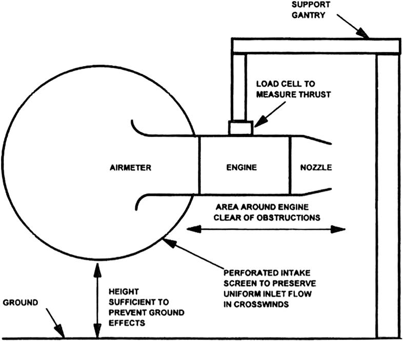
Outdoor Sea Level Thrust Test Bed
This is illustrated in Figure 10–10, and consists basically of an open air stand supporting an engine and providing thrust measurements. The effects of cross wind on entry conditions are negated by a large mesh screen fitted around the engine inlet. The immediate test bed area is free of obstructions to the airflow, to ensure the validity of the thrust and airflow readings. This is the most definitive thrust test bed, as for indoor test beds the thrust and airflow measurements are corrupted by the flow field generated by the side walls. Outdoor test beds are sited in remote areas, to minimize the environmental disturbance of the noise produced. Because of the resultant logistic difficulties and the impact of adverse weather conditions, indoor testing is preferred in most countries, with measurements calibrated versus outdoor facilities.
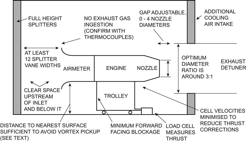
Indoor Sea Level Thrust Test Bed
Here a similar engine arrangement to that of Figure 10–10 is mounted indoors, as shown in Figure 10–11. The air flowpath to the engine is crucial, as flow disturbance must be minimized. The engine nozzle efflux enters a detuner, which exhausts hot gases and provides sound attenuation.
Note: Sea level gas generator test bed is similar but without thrust measurement.
For a given engine the measured thrust may be up to 10% less than the value that would be recorded on an outdoor test bed. This is due to unrepresentative static pressure forces acting on the engine and cradle, caused by the velocity of air within the cell passing around the engine. This air is entrained into the detuner by the ejector effect of the engine jet; it prevents hot gas reingestion and also cools the detuner. Furthermore, if the engine final nozzle is unchoked the test bed configuration can cause a rematch due to the local static pressure distribution at the nozzle exit. An indoor test bed gives useful all-weather availability, but unless the test bed is purely functional it should be calibrated against an outdoor test bed, as discussed later, to determine the effects of the static pressure field and rematch.
Key guidelines for designing an indoor test bed are presented below. These minimize the measured thrust deficiency described above, and also prevent extreme flow fields such as vortices from entering the airmeter. Owing to the complex flows within a test bed, some adjustability and subsequent experimentation may be required.
• Air should enter the test bed via a full height intake at the front, with splitters for flow straightening and noise attenuation. Additional side intakes should only be used if size constraints make them absolutely necessary.
• The distance from the inlet splitters to engine airmeter inlet should exceed a dozen splitter widths.
• Rear intakes, passing up to 10% of the main intake flow, may be employed to provide additional detuner cooling air while minimizing flow velocities past the engine.
• To avoid vortex pickup the height from the airmeter centerline to the floor or walls should exceed five airmeter throat diameters for an approach velocity of 0.01 times the throat velocity, and two throat diameters for 0.1 times the throat velocity. This may influence the choice of cell height and width.
• The space upstream of and around the airmeter should be unobstructed, to avoid flow disturbances that would impair the flow measurement.
• The air velocity within the cell flowing past the engine casing should not exceed around 10 m/s. This may also influence the cell dimensions, though it is heavily dependent on the entrained flow, which is discussed later.
• The engine cradle and slave equipment should present minimum forward facing area, to reduce thrust corrections.
• Recirculation of hot exhaust gas to the engine intake must be avoided; during test bed commissioning this should be confirmed using suitably located thermocouples.
• If the detuner turns flow vertically upwards it should incorporate a cascaded bend to minimize pressure loss.
• The detuner inlet diameter should be around three engine nozzle diameters. Increasing this increases the entrained flow.
• The axial gap between the detuner and the engine nozzle should be adjustable; values of at least two and ideally three or more engine nozzle diameters are recommended. Increasing this does not affect the entrained flow, but reduces thrust loss and rematching by avoiding pressure disturbances around the nozzle exit plane.
• The entrainment ratio, which is the ratio of entrained airflow to engine propelling nozzle flow, may be calculated from measured temperatures and a simple enthalpy balance. A good design target is 3:1 for turbojets, and lower for turbofans as engine flow is higher and discharge temperature lower.
• During test bed commissioning flow visualization using smoke should be employed as a further check on the quality of the test bed aerodynamics. This should confirm the absence of hot gas recirculation or vortex pickup, and determine suitable positions for cell static pressure measurement.
Indoor Sea Level Jet Bed or Turboshaft Gas Generator Tests
This test bed is employed when a turboshaft engine gas generator is tested with a final nozzle and exhaust detuner instead of its power turbine. The theoretical exhaust gas power is calculated based on gas generator exit flow, pressure, and temperature, and is the power that would be available from a power turbine of 100% efficiency with no duct pressure losses. Such testing is necessary when the power turbine either remains with the installation, or is supplied by another company. As this applies mainly to land-based engines, an altitude chamber would not normally be required. Key points are as follows:
• The accurate measurement of air mass flow is crucial to the power calculation. As for indoor thrust beds, flow disturbances near the airmeter must be avoided as well as vortex pickup.
• Hot gas recirculation to the intake must be avoided, as for thrust engines.
• The effect of the exhaust detuner is less critical, as the slave nozzle exit area may be “trimmed” to ensure capacity adequately matches that of the power turbine.
Indoor Sea Level Shaft Power Bed
This is used for turboprop or turboshaft engines, with output power measured directly. Figure 10–12 shows the key features of such test beds. The main differences from an indoor thrust bed are as follows.
• Air may be ducted directly to the engine from ambient rather than it flowing though the test cell, with flow measured outside the test bed at entry to the ducting. The test bed configuration does not affect measured airflow and hence measured performance; the building is only there to provide protection from adverse weather conditions.
• Alternatively air may enter the test bed through splitters and then into the engine as per a thrust bed; here test bed configuration does affect the measured airflow.
• The exhaust flow has a low velocity and is ducted directly to atmosphere with no detuner required. Entrainment effects therefore need not be considered.
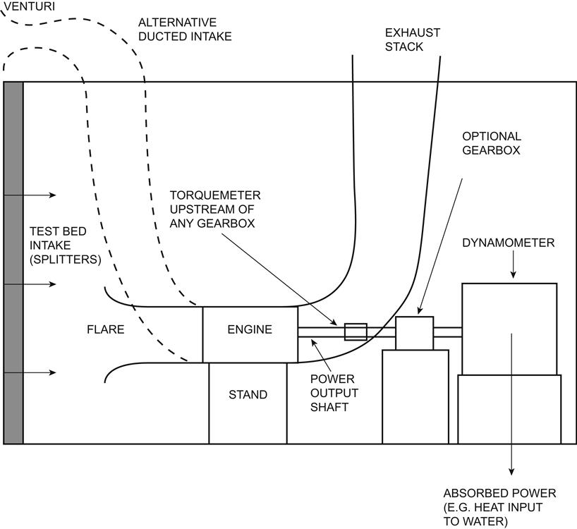
Notes: If flare is used for mass flow measurement, positioning guidelines are per Figure 10–11. Shaft power test bed has almost no entrained airflow. If a gearbox is used to match power turbine speed to dynamometer then torque/power measurement must exclude gearbox losses.
On shaft power test beds some device must absorb the engine output power, providing suitable characteristics of load versus speed. There are several possibilities:
• For a turboprop, an aircraft propeller may be fitted on the test stand.
• An alternator may be used to generate electrical power, to be either dissipated in electrical resistance banks or passed to a grid system. The latter is appealing environmentally, but usually impractical during an engine development program. Setup costs are high, rotational speed is tied to grid frequency, and intermittent operation may be unacceptable to a grid operator.
• A dynamometer absorbs power over a range of power and speed combinations, and often also measures torque. In the hydraulic type a vaned rotor and stator arrangement pumps water through the vanes. The power absorbed heats the water, which must either be cooled or a fresh supply provided. Valves control the water level within the dynamometer, which changes the power absorbed at any given speed and allows for various power/speed laws. Torque measurement utilizes a load arm and weighing system on the external casing, which is freely mounted on hearings. The input torque is transmitted via the water and any bearing friction.
Altitude Test Facility (ATF)
Thrust or shaft power test beds may be housed within an altitude test facility (ATF), which reproduces the inlet conditions resulting from altitude and flight Mach number. Figure 10–13 shows the key features of an ATF. Unlike a sea level test bed the plant must provide a continuous airflow even without the engine operating, to maintain reduced pressure and temperature.
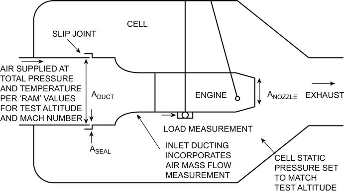
Notes: Gross thrust = Load + Aseal × (PSseal − PScell ) + Aduct × (PSduct − PScell ) + Wduct × Vduct
Nett thrust = Gross thrust − Wduct × Vduct
Wduct, load, PTduct, Tduct, PScell and PSseal are measured indirectly.
Vduct and PSduct are calculated from the measurements using Q curves.
Figure 10–14 illustrates two possible layouts of ATF plant. To simulate both ambient conditions and flight Mach number engine inlet total pressure and temperature must be controlled to the ram (free stream total) values for the altitude and Mach number. Also, the static pressure at the nozzle exit plane must be set to that of the test altitude. These parameters are mostly sub-ambient at altitude, hence common features of the various types of ATF are substantial pressure reduction, chilling and drying capabilities, and recompression of discharge air back to ambient. Accurate measurement of thrust is complex.
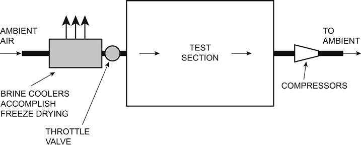

Note: Different valve settings are used depending on the pressure and temperature levels required. (Source: Rolls Royce)
The other possibility for testing at flight conditions is a flying test bed as described below, where the engine is mounted on an aircraft. The main advantages of the ATF are:
Flying Test Bed
A flying test bed is also often used for major aeroengine programs. Typically a four engined aircraft is modified to mount a single, new development engine at one berth. Compared with an ATF the advantages are:
However, as mentioned there are no direct measurements of thrust and mass flow. These must be calculated as follows.
• Propelling nozzle thrust coefficient and capacity are obtained from rig and engine tests, ideally in an ATF.
• Nozzle entry total pressure and temperature are measured directly, with sufficient coverage to obtain valid average data.
• Nozzle mass flow may now be calculated, along with exit velocity.
• Any air offtake and nacelle ejector flows are estimated from design data.
• Fuel flow is measured directly.
• Inlet airflow may now be calculated.
• Nett thrust is the difference between the total exit and inlet momentum, and if the nozzle is choked any pressure thrust must be added.
Measurements and Instrumentation
Engine tests use differing amounts and sophistication of instrumentation, depending on their purpose. Many development tests require detailed performance investigation, hence pressures and temperatures are measured at virtually every station, as well as power or thrust, shaft speeds, fuel, and airflow, etc. At the other extreme, for production pass-off or endurance testing only a minimum of measurements are taken beyond those of the production control system, such as ambient conditions, power or thrust level, and fuel flow.
This section provides background to the instrumentation used for each possible measured parameter. Indicative accuracies and coverage requirements are provided, along with a summary of how the instruments work.
Engine testing is very expensive; hence to ensure good quality data are obtained the importance of the following cannot be overemphasized.
• The test bed and all instrumentation must be properly calibrated.
• Test planning should include careful specification of instrumentation requirements.
• Key measurements must be repeatedly checked during the testing, to ensure data are valid.
• Engine removal from the test bed must be delayed, and testing repeated, if necessary.
For all of the above an understanding of likely accuracy levels is required.
Pressures
Pressures are measured for a number of reasons:
• Determination of overall engine performance requires ambient or cell pressure so that parameters can be referred back to standard conditions.
• Engine station pressures help define component performance, e.g., pressure ratios, surge margins, and flow capacities.
• Mass flow measurement is based on the local difference between total and static pressure levels.
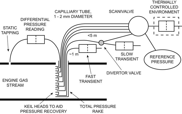
Figure 10–15 illustrates the main elements of a typical pressure measuring system. Local small holes called tappings allow the engine gas stream pressure to reach a measuring device outside the engine, via fine capillary tubes of 1–2 mm diameter. Generally at least three circumferential locations are used at a station, to increase coverage and to allow error detection by comparison of readings. A leaking line usually reads low, though thought should be given as to whether lines pass through higher pressure regions. An alternative is to gang the lines from several tappings together into a manifold and then read the manifold pressure as a pneumatic average. Though this method is relatively inexpensive a leak in any one pressure line is difficult to detect. The measuring devices used are described here.
Manometers
For pressures below around 2 bar, older test beds have used water or mercury manometers, where the height of a column of liquid in a glass tube is read visually. Small corrections are applied for the temperature of the liquid column. For a well-designed system accuracy is around 0.25%. As automatic data recording has become more prevalent manometers have virtually disappeared.
Transducers
Modern test beds use a transducer, where a pressure difference causes movement of a diaphragm, which is converted to an electrical signal. The other side of the diaphragm may be at ambient pressure or a vacuum, giving gauge and absolute readings respectively. The diaphragm movement is converted to a voltage, which is read by the data logging system. For many transducers the conversion uses an energizing voltage and a resistive straingauge on the diaphragm. Alternatives are piezo-electric, which generate their own voltage, or inductive. Calibration curves relate the electrical signal to pressure levels, and are obtained by either a dead weight tester that applies a known force and hence air pressure, or comparison with other calibrated transducers. Transducer designs are optimized for various pressure ranges; they should ensure operation is in the most linear part of the range, typically 10–90% of full scale. Transducer temperature should be controlled as this affects the straingauge resistance; even compensating circuitry does not fully eliminate the effect. Accuracies quoted herein are for a controlled transducer temperature.
Steady state, typical accuracies are around 0.1% of full scale for the basic transducer; however, a good overall accuracy is 0.5% for engine pressures. This figure allows for calibration drift, hysteresis, engine stability and pressure profiles, transducer nonlinearity, and drift in the voltage supply. Cell static pressure is less prone to engine effects, hence an accuracy of 0.25% is obtainable.
For steady state testing, many pressure tappings are read in turn via scanivalves, where rotating valvery connects a transducer to each tapping in turn. For best accuracy the transducer is kept in a temperature controlled environment, and known reference pressures are also read one or more times per scan giving continual, automatic update of the transducer calibration. With best practice overall accuracy can be around 0.25% as most transducer error effects are eliminated, leaving those due to engine pressure profiles and stability during the time taken to complete a scan. Such a system is unsuitable for transient use due to intermittent reading and volume packing of the pressure lines. The latter effect means around 4 minutes' stabilization is required before an accurate pressure reading can be obtained.
Comments on pressure measurements at the various engine stations are presented below.
Ambient Pressure—Barometers
Barometers are used to measure ambient pressure, with an accuracy of around 0.1%. They fall into two main categories:
1. An aneroid barometer consists of a dial and pointer controlled by an evacuated metal cylinder with corrugated sides and a spring action. Changes in ambient pressure cause movement which is read on the dial.
2. A mercury in glass or Fortin barometer uses a mercury column in a closed glass tube, evacuated at the closed, upper end. The height of the column is read visually.
Test Cell Static Pressure
This is required for all engines where the intake is inside a test bed, and is measured in at least two places of low cell velocity. Usual locations are on the side walls in the plane of the nozzle exit, at the same height as engine centerline. The instrumentation comprises the open end of a 1–2 mm diameter capillary tube surrounded by a perforated “pepper pot,” which removes the effects of incident velocity. The tube is then connected to either a transducer or water manometer.
Engine Static Pressures
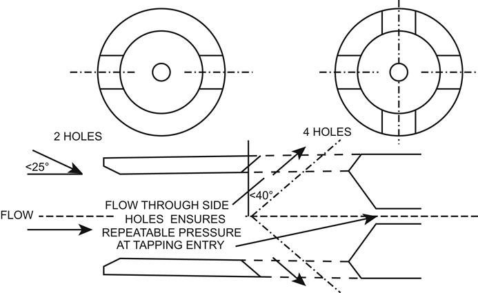
If the axis of a tapping is perpendicular to the flow direction then it will read static pressure, as no dynamic head will be recovered. Wall tappings give a more accurate reading than side or rearward facing tappings on immersed probes, as the presence of the probe disturbs the flow. Static pressure tappings may be used in place of total pressure readings if a calibration has already been obtained versus the total pressure reading. Such calibrations become tenuous, however, if there is swirl angle variation, as this changes the local Mach number.
Engine Total Pressures
To achieve full recovery of the stream dynamic head, and hence measure total pressure, the pressure tapping is mounted in a probe that points its axis towards the direction of gas flow. If the flow angle varies by more than ±5°, a Kiel head should be employed, as illustrated in Figure 10–15. This uses a chamfered entry to recover effectively the stream dynamic head for incidences of up to ±25°. Above gas temperatures of around 1300 K total pressure probes are not normally viable as they will require cooling and hence become so large that associated pressure drops are prohibitive.
Coverage requirements depend on how well understood the pressure uniformity is at a station, and should be agreed with the relevant component designer. Many radial and circumferential locations may be addressed via either multiple heads on vane leading edges, or several multihead rakes inserted into the gas stream. The heads are often placed on centers of equal flow area to assist in data averaging. Calibration of rig versus engine instrumentation standards may also be undertaken. Coverage in the cold end (compressors) should be at least three off rakes with one to five heads, depending on engine size. If large radial or circumferential non-uniformities are likely then more coverage may be employed, such as downstream of an aeroengine fan where up to 10 heads are used. For the hot end there is often significant swirl hence greater coverage may be needed. Around six rakes, or preferably instrumented vane leading edges, are suggested with two to five heads depending on engine size.
Total pressure rakes and wall static tappings may be used in combination, set in the same plane. Static tappings complete definition of the total pressure profile, as static and total pressures are equal at the walls. In addition, if the static pressure is reasonably uniform, which requires low swirl angle, the difference between total and static pressure indicates flow velocity.
Placement of total pressure rakes should consider obvious sources of error such as wakes downstream of struts. Good practice is to derive calibration factors between fitted instrumentation and that giving fuller coverage as listed above.
Differential Pressures
Normally pressure is measured as the difference between the gas stream and ambient, and an absolute pressure level obtained by addition of ambient pressure to the gauge reading. To read a pressure difference between two points, both sides of a transducer may be connected to tappings at the engine stations in question. This allows use of a more precise, lower range transducer, and avoids large inaccuracies due to the subtraction of similar numbers. One disadvantage is that recalibrating such a transducer is not possible without disconnecting the instrumentation, unlike for scanivalve systems.
Transient Pressures
For transient testing, dedicated pressure transducers, designed to optimize transient response, are required for each tapping. This provides a continuous reading, unlike a scanivalve system. The transducers are mounted local to the engine to minimize line volumes, and hence allow fast response to pressure changes; they may be water jacketed to enhance thermal stability. Line length limits are around 5 m for ordinary handling and 1 m for faster transients such as fuel spiking. In the former case a divertor valve may be employed to allow the same tapping to be read by the steady state scanivalve; for the shorter line length space does not permit this. Typical scan rates range from 10 to 500 scans per second. Absolute accuracies are lower for dedicated transient transducers than for a scanivalve system, around 1.5% of full range, and the transducers are more subject to drift.
A calibration curve should be run at the start of each working day to provide a comparison with the steady state instrumentation. In addition a transient maneuver should be performed to check for lag due to divertor valve faults.
Dynamic Measurements of Pressures
Dynamic measurements of pressure address high frequency pressure perturbations, rather than “dynamic pressure” as in the “velocity head.” These measurements are employed to detect flow instabilities such as rotating stall or rumble that can occur in the compression and combustion systems. The accuracy in determining amplitude is low, around 10% of range, as the design is optimized for response and the thermal environment is normally uncontrolled. Probes such as the kistler (resistive) and kulite (piezo) varieties are utilized, which incorporate pressure transducers—the low volume allows response to the very high frequencies involved. The kistler probe is more vulnerable to vibration but can tolerate temperatures up to 350°C, which is 80°C higher than the kulite. The signal may be available in the control room on an oscilloscope and is normally recorded in analog form on tape. Later examination of amplitudes and frequencies helps pinpoint the cause or at least onset of instability. High frequency phenomena may also be shown qualitatively by noise on ordinary transient pressure signals.
Temperatures
Measurement of temperatures provides the following information on engine and component performance.
• Determination of overall engine performance requires inlet temperature so that parameters can be referred back to standard conditions.
• The temperatures local to a component are required to define its performance, i.e., efficiency and flow capacity.
• Temperatures are required to ensure the engine is not operated beyond limits stipulated for mechanical integrity.
Temperature measurement is complex. It is vital to follow the good design and working practices outlined herein, otherwise significant inaccuracies may result.
Temperature readings more closely reflect total rather than static conditions, as a rake in the gas stream brings the gas to rest on its surface. In fact it is impossible to measure purely static temperature. The fraction of the dynamic temperature recovered is termed the recovery factor. As for pressure measurement, temperature rakes employ Kiel heads where swirl angle variation is greater than 5°, to ensure the dynamic temperature is recovered over a wide range of incident flow angles. Little error is normally incurred if rake recovery factors are taken as a constant value of 0.94, assuming well-designed probes.
Figure 10–16 illustrates the main elements of a typical temperature measuring system. The following sections describe the instruments used.
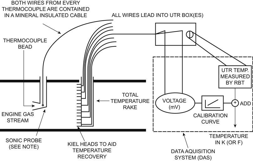
Notes: Test bed inlet temperature is measured by multiple RBTs, or on older beds a “snake.” It is not possible to measure static temperature, as most of the dynamic temperature is always recovered.
UTR = universal temperature reference
RBT = resistance bulb thermometer
Sonic probes increase heat transfer to the thermocouple by accelerating flow past the dead and to overboard. Aspirated probes use an auxiliary air ejector to accelerate flow past probe. Thermocouples may also be mounted on vane leading edges.
Resistance Bulb Thermometers (RBT)
Here temperature is measured via changes in the resistance of a heated material. Platinum is frequently used, hence the common alternative expression PRT (platinum resistance thermometer). In theory resistance thermometers are suitable for temperatures up to around 1000 K, and may give a high accuracy of potentially around 0.1 K if carefully calibrated. They are, however, comparatively delicate, and rarely used actually within an engine; the most common uses are for air inlet temperature and to measure reference temperature in thermocouple systems described later in this section.
Snakes
Snakes are resistance thermometers many meters long, sometimes used to measure average inlet temperature, and may for example be strung out over the inlet debris guard or splitter. One disadvantage is that the large physical size makes accurate calibration impossible, hence a preferred alternative is multiple resistance bulbs. Indicative overall accuracy for a snake is 1–2 K.
Thermocouples
If two dissimilar metal wires are connected at a junction, and the loose ends maintained at some reference temperature, a voltage is generated dependent on the temperature difference between the junction and the reference. Typically the junction is a welded head of up to 1.1 times the wire diameter. Thermocouples are less accurate than RBTs, but more robust. The loose ends’ temperature is maintained by either a UTR (uniform temperature reference) box, whose own temperature is measured by RBTs, or an Icell (ice cell). Single pieces of wire should be used between the hot and cold ends, otherwise measurement uncertainties increase by around 2 K per extra junction. With single pieces batch wire calibration is applicable, where a calibration is obtained of a number of thermocouples made from a particular batch of cable. Providing the results agree, this calibration is applicable to other thermocouples made from that same batch.
Thermocouples that employ different wire materials produce different voltage curves. Standard curves are defined for different thermocouple types, and different classes of thermocouple lie within different tolerances of these curves. Class 1 thermocouples will lie within the greater of 1.5 K or 0.4% of the standard curve, and class 2 within 2.5 K or 0.75%. At higher temperatures drift and hysteresis together contribute a further 3 K inaccuracy, despite heat treatment to improve thermoelectric stability. In addition typically 1 K error will be contributed by both circuitry and conduction effects around the hot junction. Combining all these effects by root sum squaring gives overall system errors at 1000 K of 5.6 K and 8.2 K for class 1 and 2 respectively. Type K thermocouples use chromel-alumel (Ni–Cr/Ni–A1) wire. Type N thermocouples (Nicrosil/Nisil, Ni–Cr–Si/Ni–Si) were introduced around 1990 to provide longer life and improved stability over type K. Overall system errors at 1000 K are reduced to 4.2 K and 7.6 K.
In sitting thermocouples radiation from adjacent surfaces must be avoided, otherwise the temperature measured is not that of the gas stream. For locations where radiation may be severe, shielded thermocouples are employed, which use up to four concentric thin tubes surrounding the thermocouple bead.
The application of the above devices to measuring temperatures at key engine stations is described below.
Air Inlet Temperature
Recommended coverage is at least three RBTs mounted on the intake debris guard, and more if non-uniform inlet temperature profiles are suspected. The test bed layout should be adjusted to ensure that the difference between the readings is less than l K, otherwise it is difficult to be sure that the true average temperature is being measured, and the temperature profile may fundamentally affect engine performance. Snakes or even thermocouples may also be used; however, this results in lower accuracy as described earlier.
Cold End (Compressor) Temperatures
Usually thermocouples are employed, and accuracy is as described earlier. Coverage should be at least three points circumferentially, with rakes having one to five heads radially depending on engine size and the expected radial temperature profile. The heads are usually placed on centers of equal area to provide uniform coverage and assist in data averaging. An aeroengine fan is a special case; due to the temperature profiles and relatively low temperature levels rakes with up to 10 heads are employed.
Hot End (Turbine) Temperatures
Temperature measurement is significantly more difficult for turbines, for two main reasons:
1. Above temperatures of around 1300 K, the mechanical integrity of a probe becomes an issue, requiring bulky, cooled designs that are highly intrusive. Such measurements are rarely attempted.
2. At combustor exit, and to a decreasing extent rearwards through a turbine system, there is severe temperature “patternation” causing both circumferential and radial profiles. This is due to having discrete fuel injection points within the combustion system and cooling air influx downstream. To obtain a thermodynamically valid average temperature from a finite number of readings may be impractical.
For both reasons the temperature at combustor exit cannot be measured, and measurements are rarely possible at exit from any first HP turbine stage. For measurement stations further downstream, the minimum coverage required is at least eight locations circumferentially, and three to five thermocouple heads radially, depending on engine size. Patternation introduces a further error beyond the thermocouple inaccuracies described above. Rather than using centers of equal area, head placement is often biased towards the walls, where the temperature gradient is steepest.
Transient Temperatures
One further important thermocouple property is response time. Physically large thermocouples take time to respond to temperature changes, due to thermal inertia, and are unsuitable for transient development testing. Response is governed mainly by the time constant of the junction itself. For development testing physically small junctions are employed, mounted to minimize conduction and radiation.
For control system instruments, large robust “production” devices are required. Here the time constant of the thermocouple can be allowed for in the control algorithms, or heat transfer increased by increasing the flow past the thermocouple junction. Where the pressure ratio to ambient exceeds around 1.2, a sonic probe is used as shown in Figure 10–16. A small flow is extracted from the gas path through a venturi surrounding the thermocouple bead and then diffuses before being dumped overboard. Otherwise aspiration is employed, where higher pressure air is injected to draw flow past the bead by an ejector effect.
Liquid Fuel Energy Flow
Measuring fuel flow fulfills two essential purposes:
1. It is vital for calculating thermal efficiency and SFC.
2. Calculating temperature levels, hence lives, of the combustor and HP turbine requires fuel flow, as these temperatures cannot be measured.
In all cases the method involves the measurement of volumetric fuel flow, conversion to fuel mass flow based on the actual fuel density, and finally deriving energy flow using the fuel heating value (FHV). To obtain the density and FHV periodic laboratory analysis of fuel samples is required. This must be done at least once per fuel batch delivery, and even each day during key performance testing. Fuel energy flow is calculated from the volumetric flow, FHV and specific gravity.
Volumetric Flow
For liquid fuels three main instruments may be used:
1. A bulkmeter measures volumetric flow over a time period, using pistons connected to a rotating crankshaft. Volumetric flow rate is directly proportional to rotational speed as this determines the rate at which the piston volumes are filled and emptied. Bulkmeters also require calibration for fuel viscosity that has a second-order effect of up to 1%. Hence fuel temperature and fuel type such as diesel or kerosene must be allowed for. Bulkmeters are almost mandatory for steady state testing and are very accurate if engine operation is stable, around 0.25% or less. They are unaffected by inlet flow profile or swirl and hence no upstream flow conditioning is required.
2. A turbine flow meter indicates instantaneous volumetric fuel flow rate, via a calibration versus rotational speed. Again fuel viscosity must be allowed for. Initial accuracy is good, around 0.5%, but drifts by up to 1%, which is more than other instrument types, due to wear on vane tips and in the bearings. Turbine flow meters are affected by inlet flow distortion, hence a minimum settling length of 10 pipe diameters must be allowed upstream, with a flow straightener such as a colander plate at the inlet to this settling length.
3. A glass bottle and stopwatch may be used for steady state testing of small engines. This involves timing the visible consumption of a known fuel volume, and gives an accuracy of around 1%. The method is not suitable for automatic data recording.
Because fuel flow is so vitally important at least two of these devices should be used in series. Figure 10–17 shows the main elements of a fuel flow measuring system, including typical installation requirements.
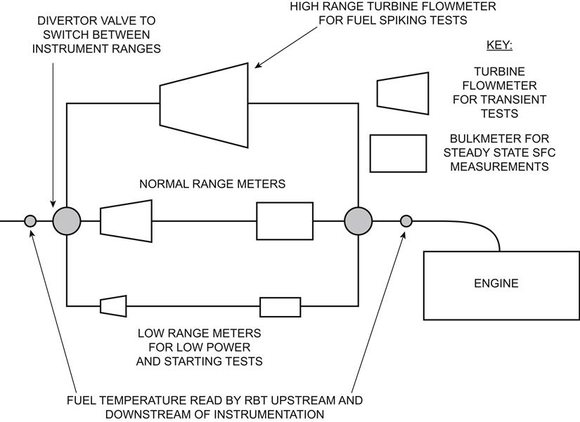
Notes: Distances between meters and pipe bends should be at least 10 pipe diameters to prevent flow disturbances from corrupting the measurements. Steady state at least two meters of some kind should be used in series to confirm the measurement accuracy. Fuel samples should be taken for analysis at least once per fuel batch and daily during key steady state testing.
RBT = resistance bulb thermometer
Turbine flow meters require upstream flow straightening, as described in the text.
Density
To measure density of a fuel sample a hydrometer is used, where a graduated scale on a float is read visually. The “units” are usually relative density or specific gravity, which is simply the ratio of the actual density (mass per unit volume) to a standard value of 1000 kg/m3. The accuracy of measurement is around 0.1%.
Actual density varies with temperature, hence temperature readings are required for both the laboratory sample test and the fuel supply to the engine. For the latter, RTBs are placed in the fuel pipes, ideally ten pipe diameters away from the flow meter to prevent possible flow disturbances corrupting the flow measurement.
Fuel Heating Value
FHV is also obtained via laboratory analysis of samples. The main methods are:
• Bomb calorimeter, in which a fuel sample is burned and the heat release measured directly from the temperature rise.
• Analysis of composition, via spectroscopy. Here the percentages of carbon and hydrogen are used to calculate the energy that would be released in combustion.
Accuracy of the above methods is around 0.1%. If no laboratory analysis is available, an FHV for kerosene only may be calculated from the density.
Transient Fuel Flow Measurement
For measuring volumetric fuel flow transiently only a turbine flow meter is suitable as its speed gives an instantaneous flow rate. The usable range is around 10–100% of full scale, so different instruments are required for starting and fuel spiking, with ranges of around 20% and 300% of that for normal running. Fuel density and lower heating value are simply the same numbers as for steady state. Both a bulkmeter and flow bottle are unsuitable as they rely on fuel flow being steady.
One backup measurement that may be particularly useful transiently is via the combustion fuel injector flow number. Given the upstream fuel pressure measurement, flow is simply the flow number times the square root of the pressure drop. This is useful during fuel spiking where fuel flow changes so quickly that even a turbine flow meter reading may lag due to inertia. The method may be checked against the main instruments based on the previous steady state position.
Gas Fuel Energy Flow
The measurement process is similar to that for liquid fuels, with fuel energy flow evaluated from volumetric flow, density, and lower heating value.
Volumetric Flow
A bulkmeter cannot be used to measure gas fuel flow as it is compressible, i.e., its density changes with pressure, and the positive displacement principle upon which a bulkmeter relies is only applicable to incompressible liquid fuels. One of two techniques is employed as outlined below.
As for liquid fuel, a turbine flow meter may be utilized, with similar installation rules and measurement accuracies. It is not necessary to calibrate for viscosity.
An orifice plate may also be utilized, and an accuracy of ±1% can be achieved. The installation criteria include a flow straightener at the measuring section inlet, and typically upstream and downstream straight lengths of pipe of 10 and 5 diameters respectively. However, orifice plates have a number of significant disadvantages relative to a turbine flow meter:
• The accuracy is only maintained for a fuel flow turn-down ratio of around 4:1, whereas for a turbine flow meter over 10:1 is common.
• The pressure drop of an orifice plate is higher, which must be allowed for in the fuel supply system.
• It is not possible to achieve the required manufacturing tolerances for engines of less than around 5 MW.
Calibration may utilize a series of sonic nozzles in parallel. This is an extremely sophisticated system and would normally be used in a laboratory rather than an engine test bed.
Density
The fact that gas fuel is compressible makes evaluation of its density complicated. The most accurate method of determining gas fuel density is from its pressure, temperature, gas constant, and compressibility. Static pressure should be the average of values measured around five diameters upstream and downstream of the volumetric flow measurement device; this upstream location is purposely after the flow straightener pressure losses. Temperature should be the average of measurements taken upstream of the flow straightener and approximately five diameters downstream of the volumetric measuring device using RTBs. For the gas constant and compressibility term (z) it is essential to analyze a sample using a gas chromatograph and then utilize formulae. The last measure is necessary as in fact very few gas supplies do not have some variability in the gas composition, and relatively small changes can significantly affect the gas constant and compressibility. Failure to do this can lead to inaccuracies of up to ±5%.
Taking all of the above measures will lead to accuracies for gas fuel mass flow of around ±1%. This is the best accuracy achievable, and is not vastly changed whether combining these effects is via root sum square (for 95% confidence) or arithmetic addition (for 100% confidence). The main inaccuracy is in volumetric flow, at best around ±0.75%, while pressure is only accurate to around ±0.25–±0.5%. Temperature has little effect, being only ±0.1 K if an RBT is used, while the compressibility and gas constant should be accurate if the formulae are used correctly.
Fuel Heating Value
The FHV can be evaluated to within 0.1% from the gas chromatograph output.
Air Mass Flow
Measurement of engine inlet mass flow is vital for various reasons:
• For thrust engines inlet mass flow determines momentum drag, and hence net thrust and SFC.
• For any engine temperature, levels in the combustor and HP turbine can only be determined by calculation from air mass flow, combustor inlet temperature, and fuel energy flow.
• Determining compressor surge margins and component flow capacities requires mass flow to be known.
• For shaft power engines tested without a free power turbine, air mass flow is required in the calculation of exhaust gas power.
Total and static pressures are read in a duct of known area, usually where contraction occurs and increases the dynamic head, along with total temperature. Measurements may also be taken at other stations, and where direct measurement is not possible calculations are performed based on flow continuity using design air system assumptions.
Airmeters
As shown in Figure 10–18, two similar instruments exist for measuring engine inlet flow:
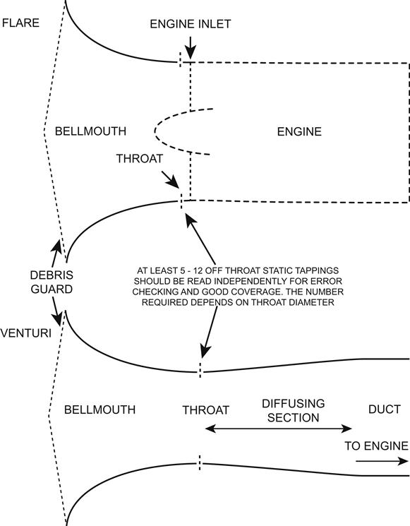
Notes: Upstream temperature measurement normally uses multiple RBTs mounted on test cell inlet splitters or debris guard. Upstream pressure measurement is either that for cell static pressure, ambient (barometric), or total probes mounted on the debris guard.
RBT = resistance bulb thermometer
Airmeter throat should be sized such that Mach number does not exceed 0.7.
1. A flare is a short duct with an entry bellmouth, fitted immediately in front of the engine. This imposes only a low-pressure drop on the engine.
2. A venturi is a contraction in a longer upstream duct, followed by a diffusing section. It is placed well upstream of any bow wave effects caused by the engine. Geometry dictates that the venturi throat generally gives a larger depression—the difference between total and static pressure—than a flare. This depression may then be more accurately measured down to low flow rates.
The term airmeter is applied to either device. Both require the use of a discharge coefficient (CD), which is the ratio of effective flow area to geometric area. This is less than unity because first, velocity is less than the ideal value, due to skin friction, i.e., total pressure is lost between the upstream measured value and the throat; and second, the flow does not fill the whole of the throat due to boundary layer growth. If the engine face is very close, such as with a flare, bow wave effects may add to this. The discharge coefficient may he determined by several possible methods:
• Cross calibration with an existing airmeter that has been calibrated on the same engine type and test bed
• Evaluation of throat conditions via a high coverage rake, with many total pressure heads
• Use of a standard airmeter geometry and CD calculation
• Theoretical predictions of flow behavior using CFD (computational fluid dynamics) methods
At least 6–12 throat static tappings should be used and read individually to allow error detection; the number depends on size. For a flare, total pressure should be that in the cell. For a venturi there may be some pressure loss upstream of the throat, hence total pressure must also be measured or the loss allowed for by calibration. Total temperature measurement ideally uses RBTs. Overall, a typical value for accuracy is around 0.5% of airflow, providing the tappings remain clean.
Turbofan Core Flow
For a turbofan the mass flow actually entering the core is of greatest interest, and may be determined in various ways.
Air System
Once a value has been established for first compressor inlet mass flow, the air system design data for cooling and leakage flows are initially assumed to obtain values for mass flows at other stations. The methods discussed under “Test Bed Analysis,” or direct measurements of individual air system flows, are used to check this assumption.
Other Measurements
For all engine stations, including entry, measurement of total and static pressures, and total temperature may provide an indicative mass flow measurement. This may be calibrated against some true measurement, either directly or using air system data depending on the location.
Transient Air Mass Flow
For transient testing a flow probe is often fitted, especially at HP compressor entry. This reads a difference between total and static pressures via a dedicated differential transducer, with short length balanced pipework to remove aerodynamic noise. The mass flow is calculated using an effective area and calibration versus steady state data based on inlet flow readings from the airmeter. If the airmeter is a close coupled flare then it may be read transiently, using dedicated transducers with 1 m or 5 m line lengths.
Injected Steam Flow
Steam may be injected into an engine to reduce emissions and increase power. The supplied steam flow must be measured directly, as least for engine development. This is normally accomplished using a vortex shedding flow meter. Here a bluff body within the flow vibrates due to shedding of wakes (just as does a telephone wire in the wind). The frequency of vibration is roughly proportional to the volumetric flow. Such a device is calibrated to determine the exact dependency, versus a choked (critical) nozzle.
Thrust
For aeroengines, measuring thrust is essential for three main reasons:
1. This is a vitally important, fundamental design goal and will determine whether or not the engine/airframe combination can meet the desired mission.
2. It is required to calculate SFC.
3. Any inferred component filing information requires a thrust level to be meaningful.
Figures 10–10, 10–11 and 10–13 showed the basic layout of sea level and altitude thrust test beds. An engine is mounted in a cradle and restrained axially via load cells, which measure the axial force required. These contain springs and are often preloaded and mounted in opposition to maintain stiffness. Standard practice is to calibrate before and after a test run, often by hanging weights, and use the mean as valid during the test. An indicative accuracy level for the load cell is within 0.25% reading; to convert this to thrust requires test bed calibration, which is discussed later. Basically, for indoor test beds the impact of the static pressure field on the engine relative to that in an infinite atmosphere must also be evaluated. This leads to an overall thrust accuracy of around 1%.
In an altitude chamber additional effects contribute to measured thrust as shown in Figure 10–13. The inlet ducting incorporates a slip joint to prevent axial force transmission to the engine; this joint has a seal area larger than the upstream duct. The actual gross thrust produced by the engine is the measured load cell force plus inlet momentum drag and pressure loads acting on the duct and seal areas. Typical accuracy is around 1.5%. For both test beds, measurement of mass flow is also important, to corroborate predictions of momentum drag at flight conditions.
Shaft Speeds
Shaft speed measurements provide valuable component information:
• Anticipated turbomachinery performance is strongly influenced by speed, especially for compressors.
• Turbine lives and shaft critical speeds are crucially dependent on speed, and for aeroengines shaft speed levels are a certification issue.
• For shaft power engines output speed is of vital importance, and is also used in the calculation of output power.
A phonic wheel and pick up are normally used. This method is highly accurate and reliable, and hence available even as a production measurement. The passing of teeth cut in a wheel, integral with the shaft, is sensed by an electromagnetic coil. The pulses generated are converted to a shaft speed, knowing the number of pulses per revolution. Two main methods may be used for this:
1. A clock and pulse counter suits steady state operation, and as implied counts the number of pulses over a timed period. Accuracy is around 0.1%, assuming engine operation is stable.
2. A frequency to DC converter suits transient operation, and gives a readout of instantaneous shaft speed. Again accuracy is around 0.1%.
Engine Output Shaft Torque and Power
These are highly interrelated as power is simply the product of torque and rotational speed.
A torquemeter forms part of a load carrying shaft, and measures torque by sensing the relative rotation of two ends of a length of shaft. Shaft torque must be measured at an appropriate point along the output shafting, as shown in Figure 10–12, to exclude any losses that are not part of the engine supply. Figure 10–19 illustrates one method where phonic wheels, which also measure speed, are attached to both the shaft and an outer unloaded tube. By this means the teeth are in the same plane, and changes in the waveform picked up indicate angular displacement, and hence torque. Overall torquemeter accuracy is around 0.5 to 1%, depending on engine stability. An alternative method utilizes strain gauges to measure shaft twist; however, such devices are delicate and have not been widely successful.
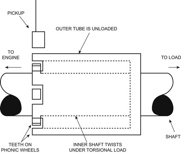
Notes: Twist of inner shaft changes angular relationship of phonic wheels. Changes in pickup waveform allow computation of shaft torque. The type illustrated is known as a “phase displacement meter.”
A hydraulic dynamometer may also measure torque. Input torque is transmitted to the casing by the water and any bearing friction; the casing is freely mounted externally on bearings to allow torque measurement via a load arm and a weighing system.
Humidity
Humidity must be measured so that test data can be referred to either dry or ISO conditions, for evaluation on a defined basis. There are three main methods of humidity measurement:
1. Capacitance sensors utilize changes in the dielectric constant of a water absorbing material.
2. Chilled mirrors utilize changes in reflected light levels as different relative humidity results in different amounts of condensation.
3. Wet and dry bulb thermometers use an air draught to evaporate water from a wet lint on one of the bulbs, and reduce that bulb’s temperature reading. Humidity is found from the temperature difference between the wet and dry bulbs, normally via tables. The traditional method was simple glass thermometers mounted on a “football rattle” frame, though ducted fans and other instruments are now used.
For all these methods an indicative accuracy level is the greater of 5% relative humidity or 0.2% specific humidity.
Geometric Parameters
Variable stator vanes are common on axial compressors, and recuperated engines often have variable turbine nozzles. To measure vane rotation directly, around three off RVDTs should be used. An RVDT is a “rotary variable displacement transformer,” in which the relative movement of electric coils changes the mutual inductance. Accuracy is good, around 0.5°, assuming all vanes are held at the same angle. If alternatively the linear displacement of the actuator moving the ring is measured, via an LVDT, then other effects are relevant, such as ring tolerances and any slack in the total mechanism. The accuracy of measured vane position is then entirely dependent on the system design.
Turbine throat areas are subject to manufacturing variation and are normally measured geometrically on build, with a repeatability of around 0.1%; method (and hence definition) adjustments may give apparent “step” changes, however. The conversion factor between area and capacity is derived from the turbine aerodynamic design data.
For thrust engines, propelling nozzle areas are required. Defining and measuring certain areas may not be trivial, for example, on a turbofan the bypass nozzle plane may contain struts, or if a mixer is employed its area is required.
Test Bed Calibration
Engine performance measured on indoor test beds will differ from that in an “infinite atmosphere.” Test bed calibration enables data from an indoor test bed to be adjusted to reflect infinite atmosphere conditions. In addition, engines of a given mark may be tested on more than one test bed, each with a different configuration and hence different calibration factors.
For shaft power engines where air is ducted from ambient as per typical installations, and the measurement made at duct entry, the test bed configuration does not normally need to be calibrated for. All that remains is the usual requirement for all instrumentation to be functioning satisfactorily.
Test Bed Definitions
Test bed approval is a formal process, involving regulation by the appropriate airworthiness authority for aircraft engines, and high customer involvement for other engine types. The following basic definitions apply, though other similar terms are also used:
• “Gold” standard test bed. This is the datum for cross calibration of all other beds for that engine type. Such calibration may be performed directly or via calibration of an intermediate “silver” standard test bed.
• “Silver” test bed. This has been directly cross calibrated against the gold standard test bed. It may be used for cross calibration of other beds for that engine type.
• “Bronze” test bed. This has been calibrated against a silver test bed. It may be used for performance testing, but not for calibrating other test beds.
• Functional test bed. This test bed has not been calibrated for performance purposes, and provides results that are indicative only. Such a test bed may be useful for endurance testing or demonstrating the functionality of a production engine, but not its performance.
A cross calibration exercise normally involves comparing results obtained running the same engine on two test beds, without any transportation of test bed slave equipment. The benefits of cross calibration are dubious for engine configurations where transportation between test beds would require significant rebuild.
Calibration of Gold Standard Test Bed
For thrust engines, the gold standard bed for the first engine of a type is declared by calibration versus an outdoor test bed, i.e., infinite atmosphere. For shaft power engines direct calibration of the mass flow measurement is required.
Steps in Test Bed Cross Calibration
The object of cross calibrating a test bed is to reproduce the performance measurements obtained on the gold standard test bed, after referral to standard conditions, such as ISA sea level static.
• All test bed instrumentation is calibrated.
• An uncertainty analysis is performed to determine the likely errors in all measurements and derived parameters accumulating from all sources. Clearly much is specific to a particular test bed.
• Calibration curves (i.e., sequences of throttle settings) are run on both test beds, consisting of around a dozen stabilized points from idle to maximum rating.
• Ideally a “1–2–1” sequence is used with the gold or silver bed as “2;” here any faults may be detected based on history. For example, the curve of inlet depression versus mass flow should be well known, and any deviation during the calibration run should be detectable. For the bed to be calibrated there may be no such history, hence having two runs proves repeatability. Other test sequences may be employed where high confidence levels make the cross calibration more of a confirmatory exercise.
• The physical configuration of the bed being calibrated is adjusted during the last test if necessary, with respect to how it affects airflow and hence thrust measurement. This includes inlet and exhaust details, engine position, and auxiliary equipment in the cell.
• Finally calibration factors are derived and are tabulated, versus speed say, for use in all future testing. These are the differences in thrust, airflow, and station temperatures and pressures.
Test Bed Audit
Test bed calibration exercises are expensive due to the engine running involved. Once a test bed has been calibrated the process is rarely repeated unless bed configuration is changed, or there is an inexplicable change in production engine performance. However, to maintain test bed approved status it should be audited, typically biannually. Important features to review in an audit are as follows:
• Trend plots of engine and overall parameters
• Instrumentation calibration status
• Original test bed calibration against a gold or silver test bed and back to infinite atmosphere
• Test bed configuration status against that formally recorded during the original calibration. Such items as physical layout, and instrumentation types and serial numbers should he examined
• Quality controls for data reduction software
• Actual working practices versus those in the engine test schedules
• Any significant events or changes noted since the previous audit
• Completion status of any “actions” from previous audits, or recorded since then
Steady State Development Testing
Specific Performance Tests
By the end of development the achieved performance standard must be demonstrated. Contractual implications mean both the customer and the engine manufacturer will be keenly interested. During development the standard is achieved via specific performance tests, which have the following aims:
• To validate the steady state performance model, or else establish which components do not achieve the predicted or rig-based bid level and hence require development effort.
• To determine the effect of component modifications implemented during a development program. Ideally these are tested singly, in a “back to back” sequence; however' this will not be the case if time is short or modifications are known to be of benefit.
• To derive control schedules for ratings and to optimize part load performance. For example, having both blow-off valves and variable vanes may allow many possible operating settings at part power for a given surge margin level.
A typical test is a performance curve consisting of around 5 to 10 stabilized points. These cover the range from the minimum power or thrust level important for the application (usually idle) to maximum rating. Stabilization times before taking readings range from around 4–20 minutes, the latter if large heat exchangers are utilized. Shorter times do not allow scanivalve pressure readings to stabilize.
For aircraft engines similar performance tests are conducted in an altitude test facility or flying test bed, to simulate the conditions encountered at cruise accurately. Owing to the time spent, altitude cruise is the most important condition for SFC.
Windmilling
For aircraft engines drag, auxiliary power capability and combustor inlet conditions are measured over a range of Mach numbers and altitudes in either an altitude test facility or flying test bed. Windmill testing is not normally conducted for other engine types.
Support of Engine Component Development
During engine development various tests are necessary where evaluating performance is not the goal but defining its level is vital to meet the primary test objective. For interest, examples of such tests are described next.
Ingestion Tests for Aircraft Engines
Ingestion events cannot be avoided for aircraft thrust engines since adequate filtration is impractical. Testing is a regulatory requirement to ensure satisfactory engine behavior, as outlined below.
• For bird ingestion tests, a number of dead birds are fired simultaneously into the engine when operating at maximum rating. The airworthiness requirements are either to maintain 75% thrust for a certain time after the impact, or shut down safely, depending on the size of bird.
• For water ingestion, the test requires static ingestion of up to 4% water, to simulate rain. However, to address the reduced fan centrifuge effect at flight speeds additional tests are normally carried out, which spray the water either at high pressure or even downstream of the fan.
• For hail ingestion, tests involve firing 25 mm and 50 mm hailstones at the engine in a specified pattern.
• At low airflows ice may build up in front of and even on the fan, and be shed and ingested; for ice ingestion the test is to ingest the ice that would build up if the anti-icing system were not switched on for 2 minutes after entering icing conditions. Ice has similar thermodynamic effects to water ingestion, but raises additional concerns about mechanical integrity.
Thermal Paint
This records the metal temperatures of key “hot end” components such as combustors and turbine blades. Special paint is applied, which changes to various colors depending on the temperature reached; several paint grades are available to suit different temperature ranges. The engine is first run at low power to heat the carcass to ensure representative seal clearances, hence cooling flows, and then held for between 3 and 10 minutes at the desired high power condition. The paint normally takes 3 minutes to cure; longer times are utilized when engine stabilization times are long, for example with a recuperated engine, though this must balance the risk of paint degradation. The paint is examined on engine strip after the test, or occasionally via borescope inspection. The indicated component surface temperatures are then related to the temperatures of the gas path and cooling air, assessed from the performance measurements and analysis.
Component Temperatures
In addition to thermal paint tests, key component areas such as disc faces may be fitted with thermocouples to measure metal temperatures. This allows the assessment of many operating conditions during a build, and provides safety monitoring during high power running or, in case of cooling flow inadequacy, in early development.
Air System
Pressure and temperature readings may be taken in key air system chambers, to validate design data for cooling flows, cooling temperatures, and pressure margins.
Straingauging
To assess the susceptibility of gas path components to resonant vibration, straingauges are cemented in key locations. These consist of fine wires embedded in a mounting plate; vibration causes the wires to stretch, which changes their electrical resistance. The test normally consists of slow acceleration and deceleration (around 4 minutes each) with various strain gauge selections being recorded. The frequency and amplitude of the measured signal characterizes blade response, identifying potentially harmful resonances. Testing explores the full range of mechanical and referred rotational speeds that the engine type will encounter. Mechanical speed determines the frequency of excitation forces, referred speed produces flow regimes that may cause excitation, and pressure level determines amplitude.
Achieving the highest speeds is often a challenge with limited test hardware, though in-service ambient variability may be addressed via an altitude chamber. Very high cycle temperatures may be reached, often requiring builds with special sizes of turbine and propelling nozzles to provide alleviation.
Bearing Loads
For this test special strain gauged equipment is built in to measure the axial loads on shaft bearings. The engine is run over a representative operating range to allow assessment of bearing lives; stabilization periods may be long (20 minutes and more) as air system pressure levels depend on seal clearances and hence disc growths.
Emissions
Exhaust gases are sampled, usually via a cruciform rake in the exhaust, and analyzed using a spectrometer for levels of pollutants such as unburned hydrocarbons, carbon monoxide, and oxides of nitrogen. Such tests are increasingly important for contractual purposes, as legislation becomes more stringent.
Endurance and Type Testing
All engines complete some form of arduous endurance test before service entry. This may take the following forms:
• Aviation authorities such as the FAA stipulate a type test comprising 150 hours’ cyclic operation, including SOT levels that are the highest that then may be permitted for any engine in service. The engine manufacturer decides this temperature level, based on hottest day/highest altitude takeoff, with allowances for engine variation, deterioration, etc. The last item in particular is flexible, but if the type test temperature gives low margins relative to new or overhauled engines, the costs of frequent maintenance will be incurred.
• For marine engines one such test has been the US Navy’s qualification test. This typically consists of 3000 hours' cyclic operation, 40% of which has the HP turbine temperature at the level required at 37.8°C (100°F) ambient temperature to achieve the power to be cleared. This level must be continually adjusted to address any deterioration, and is normally achieved during the test via “customer” bleed extraction.
• For industrial engines, testing is normally specified by the engine manufacturer, and typically comprises 100–300 hours of cyclic testing with maximum SOT 10–20 K above that at base load.
Transient Development Testing
Transient performance testing aims to confirm that the engine can perform accels and decels (known as handling) within specified times. Potential operability problems include surge and weak extinction. Before a new engine variant is tested, transient performance work will normally be based on a transient model of the engine. This is validated using transient test data and can then be used to support testing and prove transient capability at extreme conditions that are impractical to test.
Handling
The maneuvers tested exceed the most severe to be met in normal service, in order to give high confidence that engines will behave satisfactorily. Examples include:
• Fast accel, which due to overfueling gives a high HP working line.
• Slow accels and decels, defined to just avoid tripping the transient bias on handling bleeds. This gives high working lines.
• Bodie or reslam, where the engine is decelerated and then almost immediately reaccelerated. Heat soakage raises the working line beyond that of a normal accel, and also within the HP compressor drops the surge line.
• Accel following startup from cold soak conditions. This gives the highest compressor tip clearances and hence low surge lines.
During these maneuvers key parameters are measured that allow definition of speed versus time, transient working line excursions, weak extinction margins, etc. A suitable scan rate is 10–50 scans per second. For aircraft engines most work is done on sea level test beds; however, some altitude chamber or flying test bed testing is essential to verify effects at the precise conditions to be encountered.
Surge Line Measurement
Surge lines are effected by phenomena such as engine structural loads creating asymmetric tip clearances, inlet distortion, or heat soakage within the HP compressor which lowers the surge line after a decel. It may be necessary to measure actual surge lines in an engine, or at least define a surge-free region, rather than relying on rig or predicted data. Key parameters are measured so that the actual trajectory to surge can be defined. Methods of initiating surge are as follows.
For an HP compressor the most usual method is fuel spiking. Here the working line is raised by momentarily injecting excess fuel, between 100% and 400% extra over around 200 ms. A suitable scan rate is 100–500 scans per second. Either a slave rig is used, or the standard control system reprogrammed.
For LP compressors or fans the most usual method is to build a development engine with a reduced capacity LP turbine or bypass nozzle respectively, to raise the working line. Bleed extraction is used to enable stable operation at high power; the engine is then slowly decelerated until it surges. This process is repeated with various levels of bleed to map out the surge line.
Other less common techniques include in bleeding air downstream of the subject compressor, for example on small engines, or if applicable utilizing heat exchanger bypass capabilities. The first surge on a build may increase compressor tip clearance, which raises operating temperatures and lowers the surge line. These effects should be quantified by further testing, and compressors examined by borescope to check for damage. The deterioration from subsequent surges is much less.
Controller and Engine Operability Tests
Transient performance and control are inseparable. The initial control strategy and algorithms are further developed during extensive sea level and altitude testing. One particular test of interest is surge recovery, where the controller must ensure that should an engine surge for any reason in service it will recover safely. This is demonstrated during development testing via a surge induced by one of the methods described.
Starting Tests
Specific tests addressing the light up region are:
• For an air starter, per aeroengine practice, measuring crank speed versus starter supply pressure, including that available in service such as from an aircraft APU.
• Starter performance verification. With zero fuel flow, the starter is cut from steady state cranking conditions; knowing the HP shaft inertia the initial deceleration rate indicates the cranking torque.
• Exploration of a matrix of crank speeds and light up flows, identifying the light off “window” and rotating stall boundaries.
• Sensitivity to variable stator vane positions and bleed flows.
Between light up and idle, tests are required to determine the upper and lower limits of acceptable fueling. Too much fuel results in compressor stall, which is affected by the bleed and whirl levels. Too little fuel results in hang, where at low speed some limitation is reached, such as over temperature, surge or rundown. This may be explored by reducing fuel flow at various starter power levels.
For industrial, marine and automotive engines start testing is usually conducted at the prevailing ambient conditions for the sea level test bed. Problems that may arise in service on cold or hot days are then dealt with as they arise. For aircraft engines cold and hot day start tests must be included in the development program. Methods include taking the engine to a cold or hot climatic region, chilling the engine in a cold room, or using large electrical heaters at engine inlet. Furthermore altitude restart capability compliant with the windmill and starter assist envelopes must be proven by testing in an altitude test facility or flying test bed.
A further test for all engine types is a hot restart, performed shortly after shutdown with the carcass still at high temperature. As well as the effect on seal clearances, heat in the gas path lowers surge lines and raises working lines.
Engine Failure Investigation
Engine mechanical failures during development invariably have a transient dimension. In addition to any transient performance data logging, key mechanical parameters such as vibration, speeds, and pressures must be recorded either analog or at least at 1000 scans per second to cater for such an event. To avoid storing immense amounts of data it may be overwritten, say every 30 minutes.
In the event of a failure this log may be interrogated to distinguish cause and effects. One example is to determine whether a surge occurred before (and hence caused) or after (and hence resulted from) mechanical damage to a compressor. If the surge came first, the amplitude of noise or vibration with a frequency corresponding to the spool speed will increase after the step decrease in compressor delivery pressure and step increase in broad band vibration caused by the surge.
Application Testing
Further development testing is often conducted with a new engine installed in its application, prior to production release. This enables the following key issues to be addressed.
• Overall performance levels are measured in the application, as opposed to a test bed where calibration factors are required. This is particularly important for aircraft thrust engines, where test bed effects are most significant. Such testing usually has high commercial importance, as it is the final determination of whether or not the engine/airframe combination meets its performance guarantees.
• Use of “real” hardware for accessories and installation ducting, rather than any slave test bed items.
• Engine mechanical integrity faced with representative structural loads, vibration levels, ambient conditions, and operating profiles.
Production Pass Off
Production Pass Off Test
It is common practice that each engine about to be delivered to a customer, whether new production, overhauled or repair, undergoes a pass off test. The inevitable variation in manufacturing and build dimensions, even within permitted tolerances, results in variation of component and overall engine performance. A typical test sequence is as follows:
• Starting: While an unavoidable test this is nonetheless vital.
• Running in: Here rotor seals are made to cut gradually into the static linings, by say a series of increasingly rapid accelerations, extended dry cranking, or dwells at increasing power or thrust levels.
• Performance curve: Here assessments are made of SFC, thrust or power versus temperature, working lines, shaft speeds, etc.
• Handling tests: Accels and decels are carried out to prove the engine meets its specification requirements.
• Control system setup: Any required control systems stops, trims and limiters are set. Trims are adjustments to measurement signals to address engine-to-engine variations.
For practicality an exception is made for heavyweight gas turbines, however.
Acceptance Criteria
There are various limiting levels that engine performance parameters must meet for pass off. These usually include demonstration of guaranteed power or thrust without exceeding set temperature and speed limits, and achieving guaranteed SFC at this power or thrust. The acceptance criteria are usually stated at some standard conditions, to which measured data is referred. Engines may initially fail their pass off test due to faults with instrumentation or less usually with the build.
In addition to performance parameters certain mechanical integrity issues are also addressed, such as fuel leaks, vibration, oil consumption, measured temperature spread, etc.
Engine Performance Trends
Changes in component manufacture or build practice may cause increasing numbers of engines to fail the pass off test. Identifying these changes early among the general scatter is challenging. Though some special instrumentation may be fitted for the pass off test, more modern practice is to rely on that of the production control system. Instrumentation is therefore often too sparse or inaccurate to suit the conventional analysis methods. Though these may be employed additional methods are necessary, which emphasize comparison with other engines. Figure 10–20 shows an example where pass off data from a production run are plotted for LP turbine inlet temperature:
• Mass plots: These show pass off performance parameters of interest plotted versus engine number over a time period. They truly define mean engine performance and scatter, and are useful for detecting measurement errors and “rogue” engines.
• CUSUM plots: These plot the cumulative sum of the difference between each engine’s temperature (say) and an arbitrary value within its scatter band, versus engine number. Changes of slope of the mean line indicate changes of trend that may be almost impossible to detect from the mass plot.
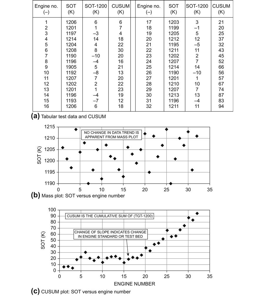
Test Data Analysis
Steps in Test Data Analysis
Test data requires considerable processing before engineering conclusions may be drawn:
1. The instrument signals must be converted from say millivolts (mV) to engineering units of K, kPa, etc.
2. Erroneous readings must be detected.
3. Where there are a number of readings at a station they must be averaged.
4. The implied performance of both the engine and individual components must be computed. An error band analysis is essential for key parameters.
5. The evaluated component and engine performance levels must be compared with expectation.
These steps do not always occur in this ideal order. Measurement errors are not necessarily easily detectable, for example they may be systematic and apply to all readings at one station. The analysis process may take a long time to “finish” as new facts alter the understanding. Furthermore, certain methods involving cycle matching combine steps 4 and 5.
Initial Error Detection and Data Averaging
It is essential before using measured data to carry out error detection, for which some techniques are listed below.
• Compare rake head readings at the same radial immersion. Low-pressure values usually indicate leaks, and any outlying temperature readings are probably in error.
• Plot readings on each rake versus immersion. This gives a finer check on validity as the “rake profiles” should show a repeatable pattern, relative both to each other and to historical data, especially for compressor rakes.
• Check that any total to static pressure ratios are sensible.
• Compare cell and barometric pressures, especially for altitude chamber tests.
• Plot airmeter static tappings versus circumferential position and compare with historical data.
• Compare fuel flow calculated from the different volumetric devices arranged in series.
• Instrumentation readings should be consistent with other readings near that station, such as from the controller or air system instrumentation.
Rake data require averaging to form a single thermodynamic mean value at each instrumented station, as represented by the performance model. Such an average is usually either area weighted or mass weighted. Mass weighting is the ideal, but as it requires an accurate knowledge of the static pressure profile, which is difficult when swirl is present, area weighting is more usual. Either way, for the average to be meaningful any faulty heads must be detected and eliminated.
Test Bed Analysis (TBA) Calculations
These compute engine and component performance levels, e.g., thrust, SFC, isentropic efficiencies, directly from the measurements. Calculations proceed sequentially through the engine, evaluating almost all parameters at each station. This requires assumptions for bleeds, pressure losses, and power offtakes. Turbine exit conditions are assessed based on work, measured in the compressors and any power offtakes.
TBA calculations may be performed either at the tested engine condition or at standard conditions such as ISA sea level or ISO. In the latter case the measurements are referred using theta (θ), delta (δ), and the appropriate non-dimensional groups. To account for variation in gas properties due to changing temperature and fuel air ratio, theta is raised to exponents other than the standard 1.0 or 0.5, known as theta exponents. The actual values are obtained by running the engine synthesis model. For illustration, Table 10–2 presents a typical range.
TABLE 10–2
Theta Exponents for Performance Data Referral
| Parameter | Theoretical Exponent | Typical Exponent |
| Temperatures | 1 | 0.97–1.03 |
| Pressures | 0 | 0.0–0.06 |
| Fuel flow | 0.5 | 0.64–0.76 |
| Shaft speeds | 0.5 | 0.48–0.50 |
| Air mass flow | 0.5 | 0.47–0.52 |
Notes:
Theta is defined as T1/288.15 K (where T1 is engine inlet temperature).
To refer measured data to standard conditions raise theta to the powers shown.
Differences between theoretical and typical values reflect changes in gas properties due to fuel air ratio and temperature changes.
Theta exponents for a particular engine type are obtained by running a thermodynamic model.
Uses of theta exponents: To convert engine performance parameters to what would be obtained at other inlet temperatures. For example, test data may be referred to standard conditions for comparison with expectation.
(Source: Rolls Royce.)
At this stage, instrumentation error detection is again essential, using the derived parameters. Errors may be detected based on considerations such as the following:
• For a fixed geometry engine with fixed bleed configuration the plot of any parameter against another should be smooth. If not, plotting both against any third parameter should indicate which reading is in error.
• Calculated component efficiencies should not exhibit high scatter, and should of course lie below 100%. Genuine hardware defects may give values below rig levels.
• Calculated component flow capacities should match any available measured values, such as based on measured throat areas.
• For a thrust engine, propelling nozzle coefficients should be uniform versus thrust level and again should resemble expectation levels.
• If an airmeter is fitted the non-dimensional flow should fall on a unique plot versus depression, be it that of the cell, engine inlet, or throat.
• Apparent “reciprocal” component changes are usually due to a single measurement error, for example the pressure or temperature between two compressors.
One special case regarding TBA calculations is a turbofan, where the core mass flow is not measured directly but must be calculated. Several methods exist, and for convenience the two most commonly used are termed methods “A” and “B” herein. Method “A” uses a core heat balance (see Figure 10–21) and method “B” employs a knowledge of HP turbine capacity. An alternative approach is a transient mass flow probe, which gives indicative rather than absolutely accurate flow measurements.
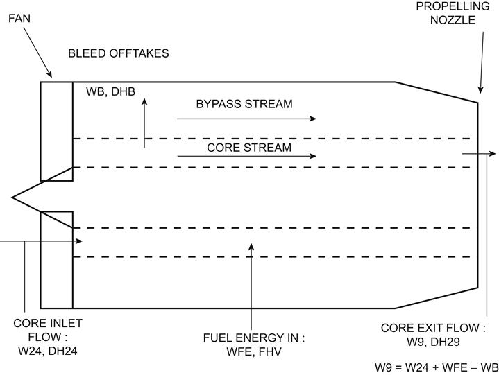
Notes: Calculate specific enthalpy from temperature and fuel air ratio. Units are kJ/kg and are typically converted to be relative to a datum of 0°C if a mean specific heat is utilized. The following parameters are measured directly: Bleed offtake flow, WB (kg/s). Fuel flow, WFE (kg/s). Core inlet and exit temperatures, T24 and T9 (K). Heat (enthalpy) balance:

Uncertainty Analysis
For key parameters produced by the TBA calculations it is essential to evaluate the likely error band resulting from the measurement uncertainty. The first step is to evaluate the potential errors in a calculated parameter resulting from that in each contributory measurement individually; the second step is to combine the effects of these errors. The most common practice is a root-sum-square addition, for 95% confidence. For 99% confidence, simple arithmetic addition is used. The process is also called error band analysis.
Comparison of Test Results with Expectation
It is usual to produce a pre-test matching model of an engine going to test. For development tests the effects of measured throat areas and any other specific hardware are normally included, whereas for a production engine the expectation—and indeed the requirement—will remain constant. It may be simply expressed via charts relating the measured parameters to thrust or power at standard conditions.
Valid comparison of the test results with expectation requires that both are based on identical conditions of inlet pressure and temperature, installation losses, etc. In addition, for contractual purposes engine performance is normally required at some standard conditions, as stated. To achieve these aims there are two main approaches:
1. Referral of measurements to standard conditions. This provides engine performance data directly usable for contractual purposes.
2. Running a synthesis model at the tested power or thrust and ambient conditions. This is more rigorous, and is mandatory for engines that do not behave non-dimensionally. In this case the model is adjusted to match the test results (see below) and run again to predict performance levels at standard operating conditions.
For both approaches the model and test parameters are plotted versus some power setting parameter. For referred data it must be in a non-dimensional form.
Evaluation of Engine Component Performance
Various methods exist for attempting to explain anomalies, which will be due to either unidentified measurement error or engine component performance differences from prediction. Test data analysis is notoriously difficult, as once dealing with “real” data the possibilities for error are vast. The various methods are described below, and should preferably be used in combination.
Traditional Methods
Engineering judgment and logical thought have long been used for test data analysis. Knowledge of what could be suspect is invaluable, and may be based on known potential causes of component deficiency, the state of engine hardware on strip, other knowledge of the test such as what checks were performed for leakage, etc. Comparison of predicted and TBA component efficiencies and capacities gives one view of component performance levels, though being vulnerable to measurement error and rematch effects it is not definitive. This traditional approach together with some trial and error may be used to determine changes to the component performance in the pre-test prediction model which allow it to reproduce all test measurements deemed valid across the power range.
Achieving alignment between a revised model and the measurements is assisted by tables of exchange rates.
Synthesis exchange rates show the change in engine performance parameters if a given component efficiency is in error by l%. Analysis exchange rates show the error in a parameter from the TBA calculations due to a 1% error in each contributory measurement. The advantages of traditional methods are that the result of such an analysis carries high credibility, as the process is easily understood, and no additional setting up is required. The disadvantage is that unlike the more automated methods described below no immediate answer is available.
Cycle Matching
Here an extended performance matching model is run at the tested conditions. It is used both to compare test data with expectation and to explain the results by changes in component performance. For test analysis the matching is extended with measurement values as additional matching constraints, and component scale factors as additional matching guesses. The model thereby changes component performance to replicate the input measurement values.
The main advantage is that analysis is performed automatically, and at the tested condition; this is more accurate than referring test data. In addition engine station data may be produced with however few measurements being taken, parameters at other engine stations being calculated based on the predicted component performance. There are some disadvantages, however. The method can only ascribe differences to component factors that are active in the matching, and the number of these is limited to the number of measurements; if some other component is at fault the answers are wrong. The matching iteration may not always work, or be ill-conditioned such that measurement errors even down to the repeatability level produce large, mutually cancelling changes in several components. Backup calculations are therefore required in online applications.
Matching methods have been successfully used by manufacturers of large turbofans and by some, though not all, airliner manufacturers. Use for industrial engines is not yet widespread.
Methods Based on Probability
Here a computer program “adjusts” both the measurement values and component performance levels so that calculated and measured station parameters match, using tables of exchange rates. By definition there is an infinite number of solutions. That given is the most likely solution, based on input values of the probability of error in components and measurements. Faced with no formal solution this gives a likely answer, and may produce useful suggestions. The solution is not unique, however, and carries little or no weight without engineering substantiation.
Transient Data
Here considerable processing is required to align instrument readings with the equivalent steady state parameters, given the reduced instrument coverage and transducer drift. Once this has been achieved, transient traces are compared with transient performance model predictions, and the model is then adjusted to achieve alignment. The model must already have a good alignment with engine steady state parameters, and adjustments are now made mainly in the modeling of heat soakage for transient operation, where real thermal masses and heat transfer coefficients are not normally known to great accuracy anyway.
Analysis/Calculations on the Effects of Water as a Vapor, Liquid, or Solid5
This section describes the effects of water in all forms—liquid, vapor, and ice—on gas turbine engine performance. When only water vapor is present, as opposed to air as well, the gas is referred to as steam. There are several reasons why water may be present in the air used by a gas turbine engine:
The above are additional to the water vapor produced by combustion. There the amount of water and carbon dioxide produced are based on fuel properties and fuel air ratio, accounted in performance calculations (see Chapter 15). The presence of any additional water beyond that produced by combustion impacts engine performance via several different effects:
• Changes in gas properties due to the presence of water vapor.
• For liquid water or ice ingestion, solid or liquid water absorbs power and affects the compressor aerodynamics, which may also lower the surge line.
• Changes in temperature due to latent heat absorption or release in ice melting or local evaporation or condensation of water.
• Increases in mass flow—for example water or steam injection into the combustor provides additional mass flow through the turbines relative to the compressors.
Performance modeling of phenomena associated with all forms of water ingestion or injection, including engine test data correction for humidity, are covered herein and relevant tables and charts are provided. For most gas turbine cycles the water vapor concentration is sufficiently low that the water/air mixture remains essentially a perfect gas. For the rare occasions where the water concentration is higher than 10% this is not so, and steam tables must be used.
Gas Properties
Three fundamental gas properties need to be considered:
Changes in Gas Properties
The presence of water vapor changes the values of these gas properties, which can have a significant effect on the thermodynamic processes throughout the engine. Both CP and R increase significantly, whilst gamma diminishes more slowly; Figure 10–22 shows the variation of these parameters versus water vapor concentration. The molecular weight of water is lower than that of dry air. Formulae 10.1–10.3 at the end of this section give the variation of CP, R, and gamma with water content.
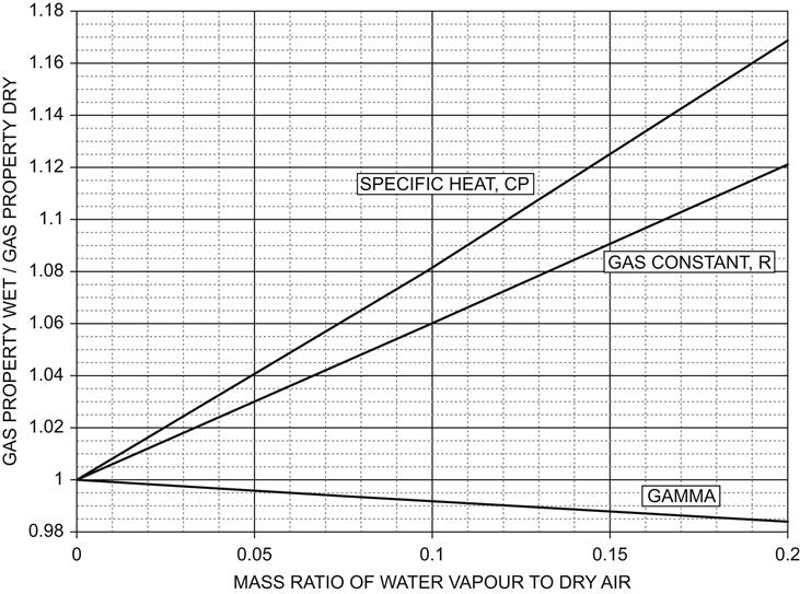
Effects on Component Performance
Engine components behave non-dimensionally and performance is mapped via various forms of parameter groups. Where the full dimensionless groups are used these maps are unique even with varying amounts of water vapor present. Quasi-dimensionless groups are also often used, where the gas properties are omitted and components mapped based on the gas properties of dry air. This form of the groups is useful as it relates the most easily observable engine parameters of flow, speed, pressure and temperature. Changes occur in these quasi-dimensionless maps due to the changes in gas properties described above. The use of such maps when water vapor is present is described in this section.
For a compressor, the presence of water vapor lowers W√T/P at constant N/√T and PR.
This is because the dimensionless group for speed, N/√(γRT), is reduced relative to dry air due to the increased R which outweighs the small reduction in γ. At this lower dimensionless speed the compressor passes a lower dimensionless flow, W√(RT)/P√γ. In addition, at this lower dimensionless flow the quasi-dimensionless flow W√T/P is further reduced, again by the increased R.
For a turbine the presence of water vapor produces little or no change in W√T/P at constant N/√T and ΔH/T. This is because, unlike a compressor, reduced speed normally either raises capacity or has no effect. One further effect of humidity is to increase the specific heat in the turbines, reducing the temperature drop for a given expansion ratio. The impact of these effects on engine performance depends on where through the engine the water is introduced.
Humidity
Description
Humidity is water vapor naturally present in the atmosphere:
• Specific humidity is the ratio of water vapor to dry air by mass
• Relative humidity is specific humidity divided by the saturated value
Effects on Engine Performance
Table 10–3 shows qualitatively the effect of humidity on leading engine parameters. Figure 10–23 presents generic exchange rates that may be utilized for first-order accuracy to predict the impact of humidity on key performance parameters. These have been derived by considering all the full non-dimensional parameter groups to be constant at a given operating condition. The impact of humidity is greater than is immediately apparent, as all parameters must be factored. For example, at a specific humidity of 0.04 (100% relative humidity on a 36°C day) shaft power increases by about 1% and LP turbine inlet temperature falls by about 1%. Hence if governing to fixed LP turbine inlet temperature the increase in power would be around three to four times this. The precise impact depends on the engine cycle.
TABLE 10–3
Humidity: Effect on Leading Performance Parameters
| Parameter | Changes At | ||
| Fixed LP Speed | Fixed Last Turbine Inlet Temperature | Fixed Power or Thrust | |
| LP speed | None | Increase | Increase |
| HP speed | Negligible | Increase | Increase |
| Mass flow | Decrease | Decrease | Decrease |
| Fuel flow | Decrease | Increase | Increase |
| Output power | Decrease | Increase | None |
| Nett thrust | Decrease | Increase | None |
| SFC | Decrease | Increase | Increase |
| Temperatures | Decrease | See note 1 | Decrease |
| Pressures | Decrease | Increase | Decrease |
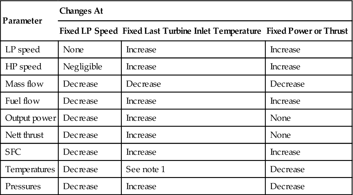
Notes: (1) Temperatures upstream of the last turbine inlet have negligible change, those downstream decrease. (2) Changes shown are for physical, not referred parameters.
(Source: Rolls Royce.)
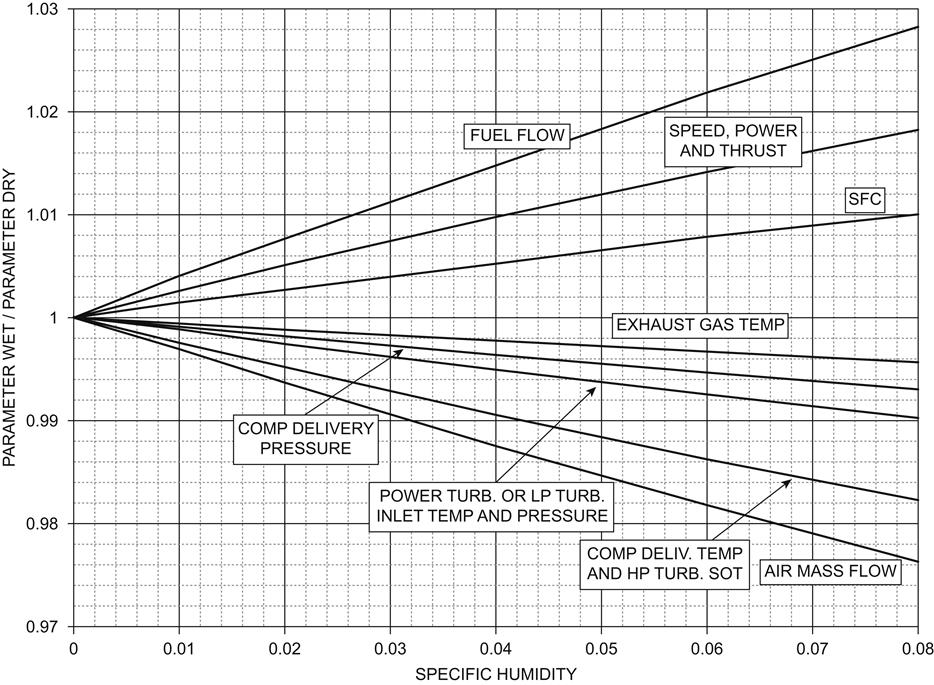
Figure 10–23 may also be used for a first-order correction of engine test data from any humidity level to that for ISO conditions:
• Divide all parameters by the relevant factor from Figure 10–23 to obtain “dry” performance
• Multiply all parameters by the factor for a specific humidity of 0.0064 (60% relative humidity at 288.15 K and 101.325 kPa)
Water Injection
Description
Water injection has been employed for both aero- and industrial engines to improve performance, utilizing one of two injection points along the gas path:
• At first compressor entry—to boost power or thrust with minimal impact on SFC. Here a relatively small amount of water is used to lower the inlet temperature by evaporation.
• Into the combustor—primarily to reduce emissions for industrial engines. This also boosts power, but makes SFC worse.
Both practices are now largely superseded by other technologies. These are increased temperature capabilities and higher bypass ratios for aeroengines, and dry low emissions combustion technology for industrial engines, where low pollutant levels are achieved without the need for water injection.
Compressor Entry Injection—Aeroengines
The takeoff condition, especially for hot days or high airfields, was particularly important for older engines with zero or low bypass ratio. Water was injected using spray nozzles, and prevented from freezing by adding methanol. The power or thrust gain primarily came from the lower inlet temperature and intercooling within the compressor rather than the additional mass flow of water. If the amount of water injected exceeded the amount that could evaporate within the compressor, further power boost was achieved by similar effects as produced by water injection into the combustor. The weight of tanks, pumps, etc., was a disadvantage, as was the need to supply purified water.
Compressor Entry Injection—Industrial Engines
Industrial engines operating in hot, arid conditions often employ an evaporative cooler upstream of the intake. This consists of a screen with water flowing over and the air flowing through it. The engine experiences a colder, more humid day, and hence can run to higher power and/or lower operating temperatures. Compared with aeroengines water consumption is lower, as only that which immediately evaporates is used. Such equipment would clearly have been impractical for aeroengines.
Combustor Injection—Industrial Engines
Water injection into the combustor has been employed to reduce NOx emissions, by lowering the temperature peaks in the combustor primary zone and hence the tendency for atmospheric nitrogen to dissociate. Side effects include increased power, but often increased emissions of carbon monoxide (CO) due to lower temperatures, especially for low-pressure ratios and short residence times. In addition combustion becomes more uneven, which may induce mechanical problems due to temperature patternation and noise. Water to fuel ratios (WFR) between 1 and 2 have been employed; as combustor temperatures are very high saturation is not a problem. The large amount of water and associated plant is a substantial disadvantage, the water being purified and pumped to the injection points via pipe work and manifolding. In addition, burners must incorporate water nozzles, and appropriate control capability is essential. As the water supply pipes etc. can be protected from low temperature no methanol is employed. SFC is worse due to the significant amount of heat required to evaporate the water.
Steam injection, described below, supplanted water injection for installations where steam plant could be used as it overcame the disadvantages associated with the chilling effect of liquid water. As stated, more modern industrial, and even marine, engines are moving instead to DLE combustion.
Effects on Engine Performance
For water injection, pumping power is not an engine performance concern, as the liquid water is incompressible and hence the power requirement is small. Logistic and weight issues of the associated plant are significant, however.
Compressor Entry
Table 10–4 shows the main effects on engine performance of water injection at compressor entry. As outlined, compressor inlet temperature is reduced by water evaporation, producing effectively a colder day and 100% relative humidity. The maximum overall performance boost at fixed SOT on a hot day is:
TABLE 10–4
Compressor Entry Water Injection: Effects on Leading Performance Parameters
| Parameter | Changes At | ||
| Fixed LP Speed | Fixed Last Turbine Inlet Temperature | Fixed Power or Thrust | |
| LP speed | None | Increase | Decrease |
| HP speed | Decrease | Negligible | Decrease |
| Mass flow | Increase | Increase | Increase |
| Fuel flow | Increase | Increase | Negligible |
| Output power | Increase | Increase | None |
| Nett thrust | Increase | Increase | None |
| SFC | Decrease | Decrease | Negligible |
| Temperatures | Decrease | See note 1 | Decrease |
| Pressures | Increase | Increase | Increase |
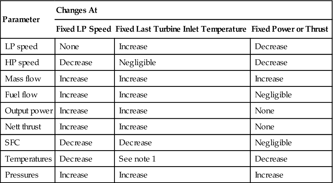
Notes: (1) Temperatures upstream of the last turbine inlet have negligible change, those downstream decrease. (2) Changes shown are for physical, not referred parameters. (3) The use of methanol as an antifreeze reduces SFC. If no liquid water persists to the combustor then this effect is slight.
(Source: Rolls Royce.)
The SFC improvement is because in non-dimensional terms the engine is suffering less from part load SFC deterioration. By coincidence the methanol prevents any increase in fuel requirement to maintain SOT (though unless liquid water persisted through to the combustor this effect would anyway be small). Saturation of the inlet air determines the feasible lowering of the inlet temperature, hence the initial humidity level has a strong limiting effect.
Figure 10–24 shows the effect on the compressor working lines, which are similar for both LP and HP compressors. At fixed mechanical speed reduced inlet temperature increases referred speed, causing operation to move further up the same compressor working line. At fixed SOT compressor referred speed increases further, again along the same working line.
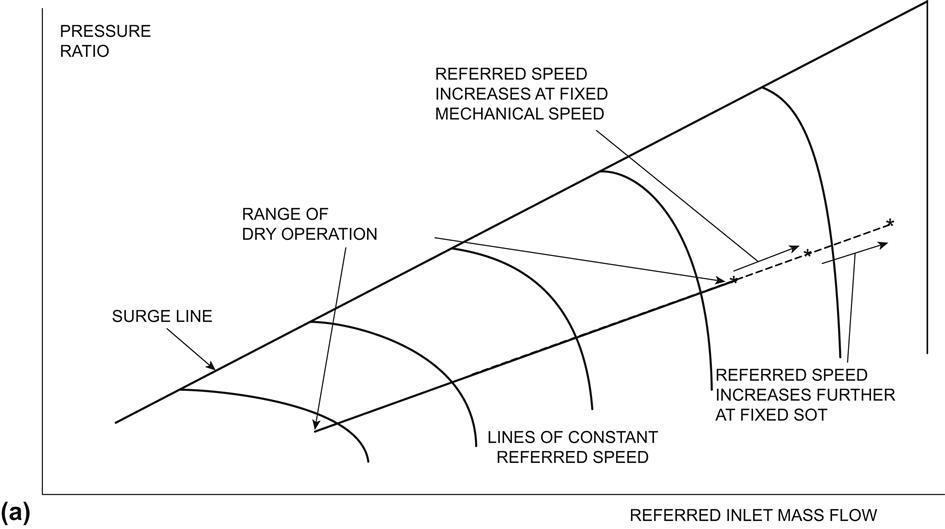
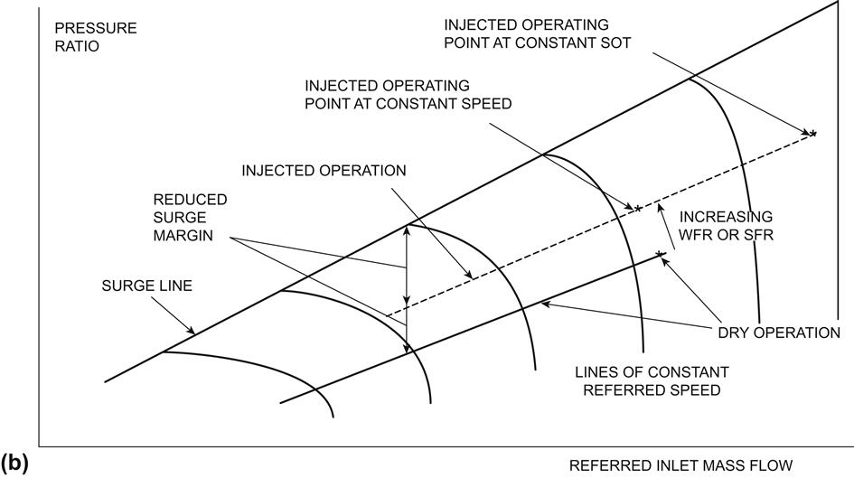
Combustor
Table 10–5 lists the effects on key engine parameters of water injection into the combustor. Typically at fixed SOT an engine with a combustor design not optimized for emissions would achieve 85% NOx reduction but with up to a three-fold CO increase. For a 1:1 WFR performance effects are:
TABLE 10–5
Combustor Water Injection: Effects on Leading Performance Parameters
| Parameter | Changes At | ||
| Fixed LP Speed | Fixed Last Turbine Inlet Temperature | Fixed Power or Thrust | |
| LP speed | None | Increase | Negligible |
| HP speed | Negligible | Increase | Negligible |
| Mass flow | Decrease | Increase | Decrease |
| Fuel flow | Increase | Increase | Increase |
| Output power | Increase | Increase | None |
| Nett thrust | Increase | Increase | None |
| SFC | Increase | Increase | Increase |
| Temperatures | Decrease | See note 1 | Decrease |
| Pressures | Increase | Increase | Increase |
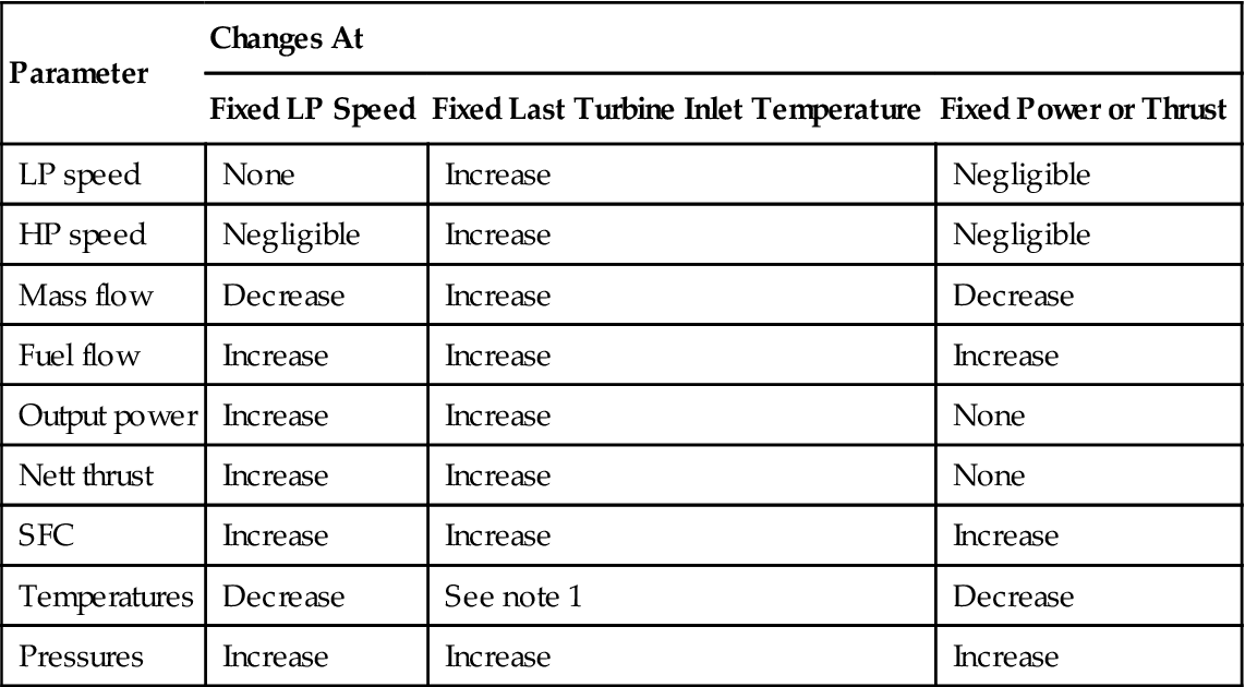
Notes: (1) Turbine temperatures decrease apart from the last turbine.
(2) Changes shown are for physical, not referred parameters. (3) The effects shown assume no use of methanol for antifreeze.
(Source: Rolls Royce.)
The increase in power output is due both to the flow in the turbines exceeding that in the compressors, and the CP of the flow in the turbines being increased by the water. The latent heat of evaporation of water requires additional fuel flow, hence the worse SFC. At fixed SOT the compressor speeds are increased along with engine inlet mass flow.
Figure 10–24 shows that in both cases the HP compressor working line is higher as the HP turbine must pass the injected water vapor flow, raising compressor pressure ratio at a referred speed to maintain the required HP turbine capacity. Because the temperature drop in the turbines is reduced, different levels of power boost are achieved depending on which turbine inlet temperature is considered constant.
Unlike steam injection, described below, water injection into turbines downstream of the H turbine is not beneficial. The large heat absorption in evaporation drastically reduces that turbine’s inlet temperature, and hence also its achievable specific power. The difference for water injection into the combustor is that extra fuel is added simultaneously, which offsets the temperature reduction due to the water. To add extra fuel to offset the temperature reduction for injection into other turbines would require impractically high temperatures in the HP turbine, or the complexity of additional combustors between the turbines.
Operability and Control Philosophy
Compressor Entry
Water injection at entry to the compressor raises few issues as it has no impact on compressor running lines, only resulting in a higher referred speed for a given SOT. The aim is to increase power while keeping within the same operating limits; compressor referred speed is increased only on occasions where it would otherwise be well below its limit. The normal control strategies of temperature and speed limits remain applicable.
Combustor
Steady state the baseline control strategy is invariably constant water fuel ratio at all power levels, and the rated power governed to the same SOT as the dry engine. However on hot and cold days the compressor mechanical or referred speed limits are reached first and the power boost is limited. In practice very cold days often already have referred speed as the limiting parameter even for the dry engine, and no power boost is possible.
Transiently, however, there are two major consequences of water injection that must be addressed by control strategies:
1. Flame out avoidance: During engine deceleration water flow is normally reduced or shut off completely. This is because the additional heat required to evaporate the water would otherwise increase the tendency for weak extinction.
2. Surge avoidance: During engine acceleration water flow is again reduced or shut off completely. Otherwise the loss in HP compressor surge margin due to the overfueling for acceleration would be too great, given the surge margin reduction due to water injection. Indeed, only by this means can the lower steady state surge margin be accepted.
Specific Engine Design for High Injection Rates into the Combustor
Water injection into the combustor beyond around 2:1 WFR would usually require reselection of turbine capacities, to prevent unacceptable surge margin or overspeed as described above. Such modification is rarely if ever undertaken, since most engines must also operate “dry.” However, both “wet” and “dry” cases may be considered in the design phase. Another item to address is increased power turbine entry temperature (PTET) at fixed SOT, due to the reduction in temperature drop in the turbine(s) driving the compressor(s).
The need for turbine capacity changes with high water injection rates arises because for the same compressor operating points compressor work is fixed, but turbine mass flow and specific heat are higher. For example, the requirements for a two shaft gas generator plus power turbine are illustrated below:
• HP turbine capacity must be increased. This accommodates the extra injected flow, preventing the rise in the HP compressor working line. It also reduces the HP turbine expansion ratio, and hence power output, to prevent an increase in HP compressor speed.
• LP turbine capacity must be decreased despite the higher mass flow, by a relatively modest amount. This forces a higher LP turbine inlet pressure, hence reducing the HP turbine expansion ratio further.
• Power turbine capacity must also be decreased, to reduce LP turbine expansion ratio, and prevent LP compressor overspeed. The lower HP and LP turbine expansion ratios are manifested as a higher power turbine inlet pressure and temperature, which give the increased engine power output.
By restagger of turbine aerofoils within casting allowances power boosts of up to 30% may be achieved for 4 WFR. As an example, at 6 WFR to retain acceptable compressor working lines and speeds the engine changes would be approximately:
Steam Injection
Description
Steam injection is employed on industrial engines to reduce NOx emissions and boost power. SFC also improves, as steam is usually raised using the engine exhaust heat, in a heat recovery steam generator (HRSG). The chilling effect of steam in the combustor is vastly less and more uniform than that of liquid water, hence there is little or no increase in CO emissions or combustion noise.
Steam injection into other turbines gives around half the SFC improvement and 1/5 of the power boost relative to the combustor, though it costs less in terms of compressor operability. Current systems have various proprietary names, such as STIG (steam injected gas turbine) or the Cheng cycle. Supplementary firing could also be employed, to increase steam production using a boiler with its own dedicated combustion.
Besides the need for steam plant and injection hardware, one significant issue for steam injection, like water injection, is the substantial need for purified water. Higher flow rates are considered than for water injection, as steam injection improves SFC. Owing to the cost and complexity of cooling towers etc. almost all systems are total loss, with the used steam simply passing up the exhaust stack. For all these reasons steam injection is employed almost solely on industrial engines rather than in mobile applications.
Effects on Engine Performance
Table 10–6 summarizes the effects of steam injection on an engine cycle. Typically an aeroderivative industrial engine at constant SOT with 2:1 steam fuel ratio (SFR) would achieve:
TABLE 10–6
Steam Injection: Effects on Leading Performance Parameters
| Parameter | Changes At | ||
| Fixed LP Speed | Fixed Last Turbine Inlet Temperature | Fixed Power or Thrust | |
| LP speed | None | Increase | Negligible |
| HP speed | Negligible | Increase | Negligible |
| Mass flow | Decrease | Increase | Decrease |
| Fuel flow | Decrease | Increase | Decrease |
| Output power | Increase | Increase | None |
| Nett thrust | Increase | Increase | None |
| SFC | Decrease | Decrease | Decrease |
| Temperatures | Decrease | See note 1 | Decrease |
| Pressures | Increase | Increase | Increase |

Notes: (1) Turbine temperatures decrease apart from the last turbine. (2) Changes shown are for physical, not referred parameters.
(Source: Rolls Royce.)
Raising steam at the highest possible temperature, dictated by the engine exhaust temperature and HRSG design, gives the best SFC; this reflects a maximum efficiency of energy recovery from the gas turbine exhaust.
In terms of component rematching the effects of steam and water injection are similar, additional power being available from the turbines due to their increased gas mass flow and specific heat. The HP turbine must pass extra flow, as for water injection, resulting in a higher HP compressor working line as per Figure 10–24. At fixed geometry the highest power boost occurs with the highest SFR that can be accepted within surge margin limits, which is normally not higher than 2.
Operability and Control Philosophy
Comments here almost exactly match those for water injection though the tendency to flame out during a decel is less for steam injection as without the need for evaporation it produces less chilling in the combustor.
Specific Engine Design for High Injection Rates into the Combustor
Almost all the same comments apply as for water injection, except that SFC improves rather than deteriorates. For a full turbine redesign, for 6:1 SFR the engine changes would be:
• Turbine capacity changes as per the 6:1 WFR water injection example above
The one difference relative to water injection is that due to the improved SFC going to high SFR is more attractive; however, as with water injection actually doing this is almost unknown in practice due to the compromise to “dry” performance.
In terms of engine cycle selection there are two other notable effects that impact the ability to produce steam:
Condensation
Description
Condensation is confined to the “cold,” compressor end of the engine and is due only to ambient humidity. The resultant water simply re-evaporates further along the gas path. Condensation may occur once flow conditions cause the local static temperature to be below the saturation value for the local water vapor partial pressure. This is determined by local static pressure and water vapor concentration; saturation corresponds to 100% relative humidity. The actual rate of condensation is determined by residence time, and by minute particles in the air that act as nuclei for water droplets. (See the discussion on the fundamental properties of the phases of water.)
In the cold end there are two regions where water vapor may condense:
1. Intake: Flow acceleration upstream of the first compressor reduces the static temperature, increasing the tendency for condensation. Figure 10–25 shows the range of humidity and local Mach number at which condensation may occur, at ambient pressure. At 40% ambient relative humidity (RH) the threshold Mach number is 0.5, and at 80% ambient RH it is 0.24.
2. Intercooler: The pressure increase in the first compressor raises the water vapor’s partial pressure. This may exceed the saturated value once the intercooler reduces the temperature. The flow velocities are low within the intercooler heat exchanger matrix to achieve the required heat transfer; this gives adequate residence time for condensation, which occurs on the cold passage surfaces. If this produces water droplets, erosion of the downstream compressor blades may be a serious problem. The important difference from water injection or rain ingestion is that intercooler condensation may continue almost indefinitely in some geographical locations, unless the degree of intercooling is reduced.
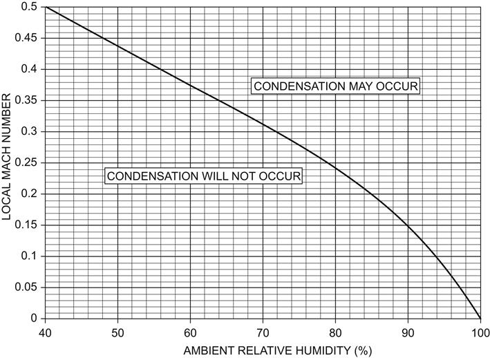
Effects on Engine Performance
Intake
Intake condensation can cause a significant change in engine performance on a test bed. The apparent loss in power or thrust and increase in SFC at fixed fuel flow may be up to 2% for hot ambient conditions, and nearer 0.5% for temperate climates. The reason for this loss in performance may not be immediately apparent, being due to pressure and temperature changes occurring downstream of test bed inlet pressure and temperature measurements. Were it possible to measure accurately the pressure and temperature actually entering the compressor then there would be negligible impact on engine referred performance relative to that without condensation. In the absence of perfect measurements or correction methods, performance testing should not be undertaken during conditions of high humidity or precipitation.
The effects of condensation are an increase in air inlet temperature and a reduction in total pressure, as well as reduced specific humidity in the initial compressor stages. The increased temperature results from the latent heat release while the pressure loss reflects the momentum change in flow acceleration due to reduced density. Once within the engine the condensed water evaporates shortly downstream.
Any engine on the test bed (or even in service) will experience a real difference in performance as referred to the engine intake lip.
Intercooler
For an intercooler system some condensation control algorithm is often employed to prevent condensation causing blade erosion downstream. The coolest air temperature must be maintained above the calculated saturation value by control of the degree of cooling. For example, for a system with an intermediate transport loop between the cold sink and the engine this may involve a partial bypass of the cold sink. The intercooler exit temperature is thereby increased, with two main consequences for engine operation:
1. Reduced LP compressor surge margin due to decreased mass flow: The reduced intercooling means the HP compressor referred speed and hence referred flow are reduced by the higher inlet temperature. In addition for a given referred HP compressor flow the actual mass flow is reduced even further.
2. Increased turbine temperatures and actual HP shaft speed: The power required to drive the HP compressor is directly proportional to its absolute inlet temperature. If this power increases, the engine must run hotter and faster to produce the same output power.
Rain and Ice Ingestion
An aircraft will encounter large amounts of rain and hail when flying through storms. Furthermore in cold conditions ice may form on the intake surfaces, occasionally breaking off to pass into the engines. Significant ingestion is normally confined to turbofans and turbojets, which must pass ingestion tests for certification as described earlier. For aero turboprop and turboshaft engines all these phenomena may be reduced by inertial separators in the intake ducts. Here airflow is drawn in around a tight bend; heavier particles fail to take this bend, passing straight on and then overboard. Industrial, automotive, and marine engines are normally protected by intake filters.
Description—Rain Ingestion
The highest rain ingestion occurs when flying through monsoon conditions. For a turbofan the fan centrifuges a significant proportion of the liquid water into the bypass duct, i.e., the rotation of the blades forces particles radially outwards. This effect is dependent on residence-time and hence is increased by wide chord fan blades and reduced by high forward speed. However, some water always passes into the core compressors.
In extreme circumstances, should liquid water persist into the combustor the heat it absorbs in evaporation has a major chilling effect. This can be a serious problem, and on the CFM56 turbofan, rain ingestion did result in several run-downs and at least one forced landing.
Description—Ice and Hail Ingestion
Icing occurs when an aircraft encounters cold cloud conditions corresponding to “freezing fog,” where air initially containing water vapor has dropped below 0°C. This causes ice to build up on the wings and engine intakes or nacelles. The ice may break off naturally when either it reaches some critical thickness, warmer air is encountered, or an anti-icing system is switched on. For engines, such a system consists of electrical or bleed air heating of the intake surfaces. The fan spinner is normally made of rubber to ensure flexibility which results in ice being shed before it has reached a dangerous thickness.
Hail is ingested simply by flying through hailstorms, the worst often being produced by a thundercloud. In either case the main issues are of mechanical integrity.
Effects on Engine Performance
Mechanical issues aside, the effects of water and ice ingestion are basically similar. Control strategies must increase fuel flow to avoid engine rundown or even flameout. Though ice has a greater chilling effect than liquid water, in practice the overall concentration is less than that of liquid water and hence this is not a major concern.
Once fuel flow is increased the thermodynamics are closer to those for combustor water injection, described above, than to compressor entry water injection. However, within the core compressors there are additional phenomena that cannot be precisely predicted:
• Water progressively evaporates through the compressors, affecting gas properties, temperature levels, and gas mass flow. It also produces an intercooling effect that is specific to the compressor type. Evaporation begins when the partial pressure and temperature cross the saturated liquid line shown at the left-hand side of Figure 10–26. It continues until the saturated vapor line is reached on the right-hand side. The rate of evaporation is also specific to a compressor type, being also strongly dependent on residence time to transfer heat to the water, and hence can only be determined empirically.
• The surge line may be lowered, due to liquid water being centrifuged outwards which affects aerodynamics at the tip section.
• Mechanical power is absorbed by the work done in accelerating liquid water through a change in swirl velocity in each compressor stage.
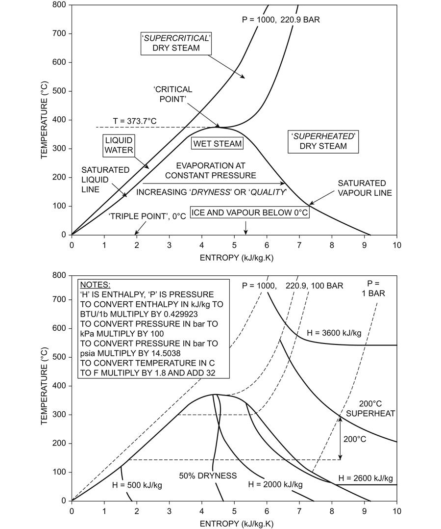
Because of the various effects, rain normally results in aeroengine testing being suspended if an important performance curve is planned. The difference between rain injection and water injection into compressors is that there the intention is to drop the inlet temperature by evaporation, and not normally to pass large quantities of liquid water through the compressors.