Geometries for CAGD
Chapter 2 describes the fundamental geometric setting for 3D modeling and addresses Euclidean, affine and projective geometry, as well as differential geometry. In the present chapter, the discussions will be continued with a focus on geometric concepts which are less widely known. These are projective differential geometric methods, sphere geometries, line geometry, and non-Euclidean geometries. In all cases, we outline and illustrate applications of the respective geometries in geometric modeling.
Special emphasis is put on a general important principle, namely the simplification of a geometric problem by application of an appropriate geometric transformation. For example, we show how to apply curve algorithms for computing with special surfaces such as developable surfaces, canal surfaces and ruled surfaces. As another example, it is shown that an appropriate geometric transformation can map an arbitrary rational surface onto a rational surface all whose offsets are also rational.
For the use of algebraic geometry in geometric design, the reader is referred to chapter 15 on implicit surfaces. We also skip difference geometry [99], which studies discrete counterparts to differential geometric properties and invariants and is thus useful in geometric computing. This holds especially for subdivision curves and surfaces (chapter 12) and multiresolution techniques (chapter 14), where discrete models of curves and surfaces play a fundamental role.
Naturally, when describing applications, we reach into many other chapters of this handbook. Thus, our references concerning applications are examples, and partially far from being complete. A much more complete picture is achieved in connection with the references in those chapters we are referring to. The addressed geometric concepts cannot be discussed in sufficient detail within the present frame. For a careful and detailed study of most of the material in this chapter we refer to the monograph by Pottmann and Wallner [94], which focusses on line geometry and its applications in geometric computing. However, it also provides the necessary classical background of related areas such as projective geometry, differential geometry, and algebraic geometry.
3.1 CURVES AND SURFACES IN PROJECTIVE GEOMETRY
Differential geometry in projective spaces requires some modifications over Euclidean differential geometry. In n-dimensional real projective space Pn, a point X is represented by a one-dimensional subspace of ![]() n+1. Any basis vector x = (x0, …, xn) in this subspace delivers the homogeneous coordinates (x0, …, xn). The latter are just defined up to a scalar multiple, and thus we write X = x
n+1. Any basis vector x = (x0, …, xn) in this subspace delivers the homogeneous coordinates (x0, …, xn). The latter are just defined up to a scalar multiple, and thus we write X = x ![]() . A parameterization of a curve c ∈ Pn is given in the form
. A parameterization of a curve c ∈ Pn is given in the form
By homogeneity, any function λ(t)c(t) with a real scalar-valued function λ(t) ≠ 0 represents the same curve. The transition from the parameterization c(t) to λ(t)c(t) is called a renormalization. Like a reparameterization, a renormalization does not change the curve as a point set. Analogously, we have to treat parameterizations of m-dimensional surfaces in Pn.
Projective differential geometry is based on properties of curves or surfaces which are invariant under reparameterization, renormalization and projective mappings. It is a very well studied classical subject [10] and turned out to be useful for various applications in geometric modeling [19]. Those include geometric continuity and local approximation with the concept of higher order contact (see [19] and Chapters 2 and 8). Other applications, which involve duality, line and sphere geometries, are outlined in the following.
As an example of a concept of projective differential geometry, we mention osculating spaces. The osculating space Γk(t0) of dimension k at a curve point c(t0)![]() is spanned by this point and the first k derivative points,
is spanned by this point and the first k derivative points,
In case that these points are not linearly dependent, one adds higher derivative points until dimension k of the spanning set is reached. Although the derivative points change both under reparameterization and renormalization, their span does not change, and thus is an example of an invariant object of projective differential geometry.
3.1.1 Bézier curves and surfaces as images of normal curves and surfaces
Rational Bézier curves are fundamental for geometric modeling. It is widely known that rational Bézier curves of degree two are conics. In fact, since polynomial Bézier curves of degree two are just parabolae, the desire to represent all types of conics, quadrics, and other important shapes such as tori exactly in a CAD system, has been one of the motivations for the introduction of the full class of rational curves and surfaces into CAGD.
The most basic algorithm for Bézier curves, de Casteljau’s algorithm, is for degree 2 equivalent to Steiner’s generation of a conic with help of two projective lines, or more precisely, ranges of points (see [27],[28],[41]). However, not only quadratic Bézier curves are deeply rooted in projective geometry. The same holds for the full class of rational Bézier curves [18]. The corresponding concept in projective geometry is that of rational normal curves [6]. These are rational curves cn of degree n which span n-dimensional projective space. Their set of osculating hyperplanes is generated by connecting associated points in n projective ranges of points. For any two different points A, B on a normal curve cn we may construct the so-called osculating simplex or fundamental simplex with vertices B0, …, Bn as follows: Point Bi is the intersection of the osculating i-space at A with the osculating (n - i)-space at B. In particular this implies B0 = A, Bn = B. The tangent at A is spanned by B0 and B1, the osculating plane at A is spanned by B0, B1, B2, and so on. Readers familiar with Bézier curves will immediately recognize the vertices of the osculating simplex as Bézier points of the curve segment defined by A and B. In fact, the segment is not yet fully defined, since the normal curve cn is (like any straight line) a closed curve in Pn. The segment is defined, if one picks an additional curve point F on the two segments defined by A and B. It is common to intersect the osculating hyperplane at F with the lines BiVBi+1 and call them frame points Fi, i = 0,…,n − 1. It can be shown that a homogeneous parameterization cn(t)![]() of cn has the form
of cn has the form
Here, bi represent the points Bi, and the homogeneous coordinate vectors bi are chosen such that bi + bi+1 represents the frame point Fi. The parameter interval for the chosen segment is [0],[1], in particular we have cn(0) = b0, cn(1) = bn, cn(0.5)![]() = F. Also just by intersecting osculating spaces, the so-called blossom can be defined and its properties may be seen as special cases of results on normal curves (see chapter 4).
= F. Also just by intersecting osculating spaces, the so-called blossom can be defined and its properties may be seen as special cases of results on normal curves (see chapter 4).
A projective map in Pn is defined if we know how it acts on the points of a simplex (say B0, …, Bn) and a further point F which is in general position with respect to the points Bi. Thus, representation (3.3) also reveals the remarkable property that any two normal curves, in fact, even any two segments of normal curves in Pn are projectively equivalent. This “standard” curve segment has no singularities, inflections, or other degeneracies in the sequence of osculating spaces.
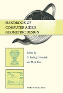
So far we have discussed normal curves, i.e., degree n curves which span Pn. Rational Bézier curves of degree n in lower dimensional spaces Pd (d < n) are obtained by applying projections of normal curves into Pd. This is illustrated for the cubic case in Figure 3.1. In fact, there we have an affine special case. A cubic polynomial normal curve c3 (normal curve with the ideal hyperplane as an osculating hyperplane) with Bézier points B0, B1, B2, B′3 is projected via a parallel projection onto the planar Bézier cubic c with control points B0, …, B3. This geometric relation between planar and space cubics can be used for a shape classification of cubics in the plane. The questions are: Given B0, B1, B2, where to choose B3 such that the curve segment has an inflection, a cusp, a loop, and so on [105]. Since the space cubic is a normal curve, it does not have such characteristics at all. Those are results of the projection and can easily be discussed with help of it (see [80],[82], where the shape analysis is extended to rational cubics and also to quartics).
A projective basis for an analogous study of triangular Bézier surfaces are the so-called Veronese manifolds [6]. As an example for the application in CAGD, W. Degen [20] discusses the types of Bézier triangles, especially those of degree two. His characterization of quadrics is a basis for further work on quadric patches by G. Albrecht [2].
3.1.2 NURBS curves and surfaces in projective geometry
As we have seen, the notion of a frame point, which goes back to G. Farin [26], is important for a geometric input of a rational Bézier curve. The so-called weights (the homogeneizing coordinates x0 of the control points, see chapter 5) have the disadvantage of not being projectively invariant. There is another advantage of frame points. With help of them, we may form a geometric control polygon of a rational Bézier or B-spline curve in projective space as follows: On each straight line BiBi+1 connecting consecutive control points take that segment as member of the geometric control polygon, which contains the frame point Fi (see Figure 3.2).
Frame points are tied to the curve in a projectively invariant way: Assume a rational Bézier curve c(t) with geometric control polygon B0, F0, B1, F1, …, Bn. A projective transformation ![]() maps c(t) to a rational Bézier curve c′(t) whose geometric control polygon is
maps c(t) to a rational Bézier curve c′(t) whose geometric control polygon is ![]() . An analogous property holds for rational B-spline curves.
. An analogous property holds for rational B-spline curves.
An advantage of the use of the projective control polygon is that we do not have to confine ourselves to positive weights when formulating the most fundamental shape property, namely the variation diminishing property. In the projective setting, it reads as follows: A hyperplane H intersects a NURBS curve c(t) (not contained in H) in at most as many points as it intersects the geometric control polygon of this curve, if no vertex has zero weight.
Frame points (also referred to as Farin points) for rational Bézier triangles have been introduced by G. Albrecht [1].
Projective geometry enters many algorithms for rational curves and surfaces, such as reparameterization, degree elevation and shape modification. For those topics, the reader is referred to chapter 5 of this handbook and to [27],[28],[41],[77] and the references therein.
3.1.3 Duality and dual representation
The Bézier representation of a rational curve expresses the polynomial homogeneous parametrization c(t)![]() in terms of the Bernstein polynomials. Then the coefficients have the remarkable geometric meaning of control points with a variety of important and practically useful properties.
in terms of the Bernstein polynomials. Then the coefficients have the remarkable geometric meaning of control points with a variety of important and practically useful properties.
The tangent of a planar rational curve c(t) = c(t)![]() at t = t0 is computed as the line which connects c(t0) with its first derivative point c1(t0) = ċ(t0)
at t = t0 is computed as the line which connects c(t0) with its first derivative point c1(t0) = ċ(t0)![]() . It has the homogeneous line coordinate vector
. It has the homogeneous line coordinate vector ![]() u(t) =
u(t) = ![]() (c(t) Λ ċ(t)). Thus the family of tangents has again a polynomial parametrization, which can be expressed in the Bernstein basis. This leads to a dual Bézier curve
(c(t) Λ ċ(t)). Thus the family of tangents has again a polynomial parametrization, which can be expressed in the Bernstein basis. This leads to a dual Bézier curve
which can be seen as a family of lines in the (ordinary) projective plane, or as a family of (ordinary) points of its dual plane. For the concept of projective duality, see section 2.5 of chapter 2.
The family of tangents of a planar rational Bézier curve is a dual Bézier curve, and vice versa.
When speaking of a Bézier curve we often mean a curve segment. In the form we have written the Bernstein polynomials, the curve segment is parametrized over the interval [0],[1]. For any t ∈ [0],[1], Equation (3.4) yields a line U(t) = ![]() u(t). The original curve segment is the envelope of the lines U(t), where t ranges in [0],[1].
u(t). The original curve segment is the envelope of the lines U(t), where t ranges in [0],[1].
As an example of dualization, let us discuss the dual control structure of a Bézier curve c (see Figure 3.3): There are the Bézier lines Ui = ![]() ui, i = 0,…, m, and the frame lines Fi, whose line coordinate vectors are given by
ui, i = 0,…, m, and the frame lines Fi, whose line coordinate vectors are given by
Frame line Fi is concurrent with the Bézier lines Ui, and Ui+1. This is dual to the collinearity of a frame point with its two adjacent Bézier points.
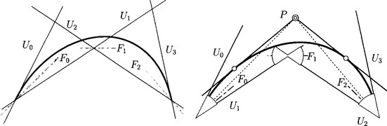
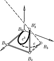
Figure 3.3 Left: Dual Bézier curve. Right: Complete dual control structure and variation diminishing property.
We could also use weights instead of frame lines, just as we could have used weights instead of frame points. Because weights are no projective invariants, it is preferrable to use frame lines and frame points. An invariant statement of theorems is also important for their dualization.
For a Bézier curve, the control points B0 and Bm are the end points of the curve segment, and the lines B0VB1 and Bm−1VBm are the tangents there. Dual to this, the end tangents of a dual Bézier curve are U0 and Um, and their points of contact are given by U0 ∩ U1 and Um−1 ∩ Um, respectively.
We dualize the geometric control polygon: The line pencil spanned by lines Ui and Ui+1 is divided into two subsets, bounded by Ui and Ui+1. The one which contains the frame line is part of the complete dual control structure (see Figure 3.3).
Dual to the variation diminishing property of a rational Bézier curve with respect to its projective control polygon we can state the following result: If c is a planar rational Bézier curve, the number of c’s tangents incident with a given point P does not exceed the number of lines of the complete dual control structure which are incident with P (if no control line has zero weight).
This result easily implies a sufficient condition for convexity of a dual Bézier curve. By a convex curve we understand part of the boundary of a convex domain. A support line L of a convex domain D is a line through a point of the boundary of D such that D lies entirely on one side of L. Now the convexity condition reads: If the Bézier lines Ui and the frame lines Fi of a dual Bézier curve c are among the edges and support lines of a convex domain D, and the points Ui ∩ Ui+1 are among D’s vertices, then c is convex and lies completely outside D.
A planar rational curve segment, or more precisely, a rational parameterization of it, possesses two Bézier representations: the usual, point-based form, and the dual line-based representation. There are simple formulae for conversion between the two forms (see, e.g., [79],[83],[94]). However, their behavior when used for design purposes is different. By using the standard representation it is difficult to design cusps but quite easy to achieve inflections of the curve segment. In the dual representation, very special conditions on the control structure must be met to design an inflection, but it is easy to get cusps. This is illustrated by Figure 3.4. For many applications, cusps are not desirable and therefore the convexity condition plays an important role. To achieve inflections, it is best to locate them at end points of the Bézier curve segments (see [79]). Cusps and inflections are dual to each other, but cusps are sometimes easier to detect than inflections. This has been the motivation for J. Hoschek [39],[40] to introduce duality and dual Bézier curves and surfaces to CAGD.
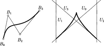
Figure 3.4 Standard control structure tends to generate inflections, whereas the dual control structure tends to introduce cusps.
The dual representation also provides an advantage in the construction of rational curves and surfaces with rational offsets, which will be outlined below in connection with the use of Laguerre sphere geometry.
3.1.4 Developable surfaces as dual curves
Dualizing the point set of a curve in 3-space, we obtain a family of planes, whose envelope is a developable surface. A developable surface is characterized by the property that it can be mappedare isometrically into the plane. Because such surfaces can be unfolded into a planar surface without stretching or tearing, they play an important role in various applications, e.g., in sheet-metal and plate-metal based industries.
Dual to the tangents of a curve, a developable surface carries a one-parameter family of lines (rulings), and thus it is a ruled surface. The rulings may pass through a fixed finite or ideal point; this characterizes general cones or cylinder surfaces, respectively. The rulings may also be the tangents of a space curve c. On such a tangent surface, the curve c itself is singular and called curve of regression. More general developable surfaces are composed of segments of the mentioned basic types.
It turned out that for the design of developable NURBS surfaces the use of the dual representation has an advantage over treating them as ruled surfaces. This is so, since a ruled surface, represented as a tensor product Bézier or B-spline surface of bidegree (1, n) has to fulfil a very special condition in order to be developable: the tangent plane has to be constant along any of its rulings. This results in a nonlinear system for the control points, whose general solution is difficult to obtain [3],[52].
To construct developable Bézier or general NURBS surfaces, one applies duality in P3 to Bézier or NURBS curves, respectively. Hence, we obtain a dual control structure consisting of control planes and frame planes, whose major properties follow by duality, just as in the case of dual Bézier curves in the plane. Conversion of a NURBS developable surface from the dual form to its standard representation as a tensor product surface, interpolation and approximation algorithms (see also section 3.4.2 and Figure 3.14), the treatment of singularities, and other topics have been studied [9],[13],[15],[42],[43],[56],[60],[83],[93],[94].
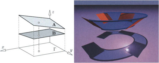
Figure 3.14 Left: To the definition of the deviation of two planes: Right: Developable surface approximating four planes.
Developable surfaces with creases, e.g. models of crumpled paper, are discussed in [4],[48]. The dual representation of developable surfaces also appears in the computation of envelopes [47],[113],[114]. Finally, even in certain algorithms for non-developable ruled surfaces, the dual representation may have some advantages [44].
3.2 SPHERE GEOMETRIES
In projective geometry the basic geometric elements are points and hyperplanes with incidence as their fundamental relation. Many geometric methods and properties involving (Euclidean) spheres are represented more elegantly, though, if one uses sphere geometries, i.e., spheres by themselves are the basic geometric elements. Classical sphere geometries include Laguerre geometry and Möbius geometry, both of which can be embedded in a larger concept, namely Lie geometry. For a detailed treatment of classical sphere geometries we refer to [5],[8],[17],[12],[67]. One of the most recent applications of sphere geometries can be found in biogeometric modeling [24], namely the concept of molecular skin surfaces [23].
3.2.1 Models of Laguerre geometry
The fundamental geometric elements of Laguerre geometry in Euclidean n-space En are oriented hyperplanes and oriented hyper spheres. Let H denote the set of oriented hyperplanes H H of En and C the set of hyperspheres C including the points of En as (non-oriented) spheres with radius zero. The elements of C are called cycles. The basic relation between oriented hyperplanes and cycles is that of oriented contact. An oriented hypersphere is said to be in oriented contact with an oriented hyperplane if they touch each other in a point and their normal vectors in this common point are oriented in the same direction. The oriented contact of a point (nullcycle) and a hyperplane is defined as incidence of point and hyperplane.
Laguerre geometry is the survey of properties that are invariant under the group of so-called Laguerre transformations α = (αH, αC) which are defined by the two bijective maps
which preserve oriented contact and non-contact between cycles and oriented hyperplanes.
Analytically, a hyperplane H is determined by the equation u0 + u1x1 + … + unxn = 0 with normal vector (u1,…,un). The coefficients ui are homogeneous plane coordinates (u0, …, un) of H in the projective extension Pn of En. Each scalar multiple (λu0,…, λun), λ ∈ ![]() {0} describes the same hyperplane. Thus it is possible to use normalized homogeneous plane coordinates
{0} describes the same hyperplane. Thus it is possible to use normalized homogeneous plane coordinates
which are appropriate for describing oriented hyperplanes. The unit vector (u1,…,un) determines a unit normal and the orientation of the hyperplane.
is determined by its midpoint m = (m1, …, mn) and signed radius r. Positive sign of r indicates that the normal vectors are pointing towards the outside of the hypersphere, whereas in the case of negative sign of r they are pointing into the inside. Points of En are cycles characterized by r = 0.
The relation of oriented contact is given by
Another model of n-dimensional Euclidean Laguerre space can be constructed in n + 1-dimensional affine space ![]() n+1, by using the cyclographic mapping ζ:
n+1, by using the cyclographic mapping ζ: ![]() n+1 → C. It maps points x = (m1, …, mn, r) to cycles C = ζ(x) with midpoint m = (m1, …, mn) and oriented radius r. If x = (m1,…, mn, 0), ζ(x) gives the point (nullcycle) m.
n+1 → C. It maps points x = (m1, …, mn, r) to cycles C = ζ(x) with midpoint m = (m1, …, mn) and oriented radius r. If x = (m1,…, mn, 0), ζ(x) gives the point (nullcycle) m.
A geometric interpretation of the mapping ζ can be given as follows (see Figure 3.5 for dimension n = 2): We assume Euclidean n-space En to be embedded as the hyperplane Π: xn+1 = 0 in ![]() n+1. Let Γ(x) denote a hypercone of revolution with vertex x, whose axis is parallel to the xn+1-axis and whose generators enclose the angle γ = Π/4 with the xn+1-axis. Such cones will be called γ-cones, henceforth. Then the cycle ζ(x) is the intersection of Π with Γ(x), where one has to add the correct orientation according to the sign of the n + 1-th coordinate of x.
n+1. Let Γ(x) denote a hypercone of revolution with vertex x, whose axis is parallel to the xn+1-axis and whose generators enclose the angle γ = Π/4 with the xn+1-axis. Such cones will be called γ-cones, henceforth. Then the cycle ζ(x) is the intersection of Π with Γ(x), where one has to add the correct orientation according to the sign of the n + 1-th coordinate of x.
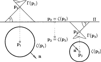
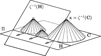
Now we focus on oriented contact of cycles and oriented hyperplanes (see Figure 3.6 for n = 2). The ζ-preimage of all cycles C being in oriented contact with a fixed hyperplane H = (u0, …, un) are the points x of a hyperplane ζ−1(H): u0+u1x1 + … + unxn + xn+ 1 = 0, according to (3.7). This hyperplane is incident with H and encloses an angle of γ = Π/4 with Π. It is called a γ-hyperplane. A γ-hyperplane touches the γ-cones Γ(x) of its points x along generators of γ(x), which will be denoted by γ-lines.
We summarize: The cyclographic mapping ζ maps points of ![]() n+1 to cycles C of Euclidean Laguerre n-space. Hyperplanes in
n+1 to cycles C of Euclidean Laguerre n-space. Hyperplanes in ![]() n+1 with inclination angle π/4 to π correspond to oriented hyperplanes H. Incidence of point and γ-hyperplane in
n+1 with inclination angle π/4 to π correspond to oriented hyperplanes H. Incidence of point and γ-hyperplane in ![]() n+1 is equivalent to oriented contact of the corresponding cycle and oriented hyperplane.
n+1 is equivalent to oriented contact of the corresponding cycle and oriented hyperplane.
In the cyclographic model ![]() n+1, Laguerre transformations (3.6) appear as transformations of
n+1, Laguerre transformations (3.6) appear as transformations of ![]() n+1 which transform γ-lines to γ-lines. This is already sufficient to classify these transformations as special affine maps
n+1 which transform γ-lines to γ-lines. This is already sufficient to classify these transformations as special affine maps
where Epe = diag(1, …, 1, −1). Formula (3.8) describes similarities in a pseudo-Euclidean geometry (also called Minkowski geometry). Its metric is based on the scalar product
Points p and q with ≶p, q![]() pe = 0 correspond to cycles ζ(p), ζ(q) which are in oriented contact.
pe = 0 correspond to cycles ζ(p), ζ(q) which are in oriented contact.
Besides the cyclographic model of Euclidean Laguerre space, which represents cycles by points, there are further geometric models, which give a point model for the set H of oriented hyperplanes.
By dualizing the cyclographic model, γ-hyperplanes (representing the oriented hyperplanes of Euclidean Laguerre n-space) are mapped to points on a quadratic hypercone in ![]() n+1, the so-called Blaschke hypercone Λ. Points of the cyclographic model (representing cycles) are mapped to hyperplanar intersections of Λ. The Blaschke model of Euclidean Laguerre space thus is just the dual of the cyclographic model.
n+1, the so-called Blaschke hypercone Λ. Points of the cyclographic model (representing cycles) are mapped to hyperplanar intersections of Λ. The Blaschke model of Euclidean Laguerre space thus is just the dual of the cyclographic model.
A stereographic projection of the Blaschke cone Λ into a hyperplane ![]() n yields the so-called isotropic model of Euclidean Laguerre n-space. Oriented hyperplanes H ∈ H are represented by points in
n yields the so-called isotropic model of Euclidean Laguerre n-space. Oriented hyperplanes H ∈ H are represented by points in ![]() n, cycles C ∈ C are given as special quadrics in
n, cycles C ∈ C are given as special quadrics in ![]() n, which are spheres with respect to an isotropic metric in
n, which are spheres with respect to an isotropic metric in ![]() n; cf. section 3.5.3. A detailed discussion of the Blaschke model and the isotropic model, including their analytic treatment and applications to CAGD, can be found in [53],[74],[87].
n; cf. section 3.5.3. A detailed discussion of the Blaschke model and the isotropic model, including their analytic treatment and applications to CAGD, can be found in [53],[74],[87].
3.2.2 Möbius geometry
Let En be real Euclidean n-space, P its point set and M the set of (non-oriented) hyperspheres and hyperplanes of En. We obtain the so-called Euclidean conformal closure EnM of En by extending the point set P by an arbitrary element (ideal point) ∞ ∉ P to PM = P ∪ {∞}. As an extension of the incidence relation we define that ∞ lies in all hyperplanes but in none of the hyperspheres. The elements of M. are called Euclidean Möbius hyperspheres.
Euclidean Möbius geometry is the study of properties that are invariant under Euclidean Möbius transformations. A Möbius transformation is a bijective map of PM, which maps Möbius hyperspheres to Möbius hyperspheres. A simple example is given by the inversion x ![]()
![]() with respect to the sphere x2 = r2 in
with respect to the sphere x2 = r2 in ![]() n. Another example is the reflection at a hyperplane, viewed as Möbius sphere. Any general Möbius transformation is a composition of inversions with respect to Möbius spheres.
n. Another example is the reflection at a hyperplane, viewed as Möbius sphere. Any general Möbius transformation is a composition of inversions with respect to Möbius spheres.
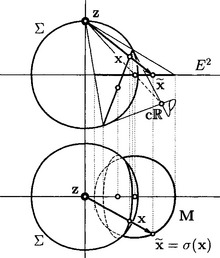
Besides the standard model of Euclidean Möbius geometry, mentioned above, we obtain the quadric model of this geometry by embedding En in Euclidean n + 1-space En+1 as plane xn+1 = 0. Let σ: ∑ {z} → En be the stereographic projection of the unit hypersphere
onto En with projection center (or north pole) z = (0,…, 0, 1), see Figure 3.7.
Extending σ to ![]() with
with ![]() : z
: z![]() ∞gives the quadric model of Euclidean Möbius geometry which is related to the standard model via
∞gives the quadric model of Euclidean Möbius geometry which is related to the standard model via ![]() . The point set is that of ∑ ⊂ En+1 and the Möbius spheres are the hyperplanar intersections of ∑ since σ is preserving hyperspheres.
. The point set is that of ∑ ⊂ En+1 and the Möbius spheres are the hyperplanar intersections of ∑ since σ is preserving hyperspheres.
For the analytic treatment of Euclidean Möbius geometry, let ![]() denote a point in En, and
denote a point in En, and ![]() the corresponding point of ∑ ⊂ En+1. Let Pn+1 denote the projective extension of En+1. In homogeneous coordinates we then have x
the corresponding point of ∑ ⊂ En+1. Let Pn+1 denote the projective extension of En+1. In homogeneous coordinates we then have x ![]() = (x0, x1,…, xn+1)
= (x0, x1,…, xn+1)![]() with -x20 + x21 + … + x2n+1 = 0 (x
with -x20 + x21 + … + x2n+1 = 0 (x ![]() ∈ ∑). The inverse stereographic projection σ−1: P → ∑{z} ⊂ En+1 is given by
∈ ∑). The inverse stereographic projection σ−1: P → ∑{z} ⊂ En+1 is given by
The homogeneous coordinates x = (x0,x1,…,xn+1) are called n-spherical coordinates of a point ![]() . These coordinates are appropriate to represent Möbius spheres as well: Via σ−1 a Möbius sphere M ∈ M corresponds to a hyperplanar intersection of ∑, whose pole with respect to ∑ shall be denoted by c
. These coordinates are appropriate to represent Möbius spheres as well: Via σ−1 a Möbius sphere M ∈ M corresponds to a hyperplanar intersection of ∑, whose pole with respect to ∑ shall be denoted by c ![]() , see Figure 3.7. Its homogeneous coordinates
, see Figure 3.7. Its homogeneous coordinates
are called the n-spherical coordinates of M. For n = 2,3 these coordinates are usually denoted by tetracyclic and pentaspherical coordinates, respectively.
It can be easily verified that in case of c0 = cn+1 the Möbius sphere M represents a hyperplane of the standard model with equation -c0 + c1x1 + … + cn+1xn+1 = 0. In case of c0 ≠ cn+1 the Möbius sphere M represents the hypersphere with midpoint 1/(c0 - cn+1) ˙ (c1,…,cn) and radius (c21 + … + c2n+1 - c20)/(c0 - cn+1)2. Let
with EM = diag(-1, 1,…, 1) describe an indefinite scalar product. Then we are able to describe points by n-spherical coordinates x with 〈x, x〉M = 0 and Möbius spheres by n-spherical coordinates c with 〈c, c〉M > 0. Incidence of a point x ![]() and a Möbius sphere c
and a Möbius sphere c ![]() is given by 〈x, c〉M = 0.
is given by 〈x, c〉M = 0.
It is a central theorem of Euclidean Möbius geometry that in the quadric model all Euclidean Möbius transformations are induced by linear maps Pn+1 → Pn+1,x ![]() A ˙ x with AT ˙ EM ˙ A = λEM, where Pn+1 again denotes the projective extension of En+1. These linear maps represent those projective maps of Pn+1 that keep ∑ fixed (as a whole).
A ˙ x with AT ˙ EM ˙ A = λEM, where Pn+1 again denotes the projective extension of En+1. These linear maps represent those projective maps of Pn+1 that keep ∑ fixed (as a whole).
3.2.3 Applications of the cyclographic image of a curve in 3-space
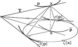
With help of the cyclographic mapping, the points of a curve p in ![]() 3 are mapped to a family of cycles in the plane E2. The envelope of this family of cycles is called the cyclographic image c(p) of the curve. Points of the envelope can be constructed with help of the tangents of p as shown in Figure 3.8. Note that the orientation of cycles in planar Laguerre geometry can be visualized by a counterclockwise (positive) or clockwise (negative) orientation of the corresponding circle.
3 are mapped to a family of cycles in the plane E2. The envelope of this family of cycles is called the cyclographic image c(p) of the curve. Points of the envelope can be constructed with help of the tangents of p as shown in Figure 3.8. Note that the orientation of cycles in planar Laguerre geometry can be visualized by a counterclockwise (positive) or clockwise (negative) orientation of the corresponding circle.
Consider a Bézier curve p in ![]() 3 all of whose control points bi are contained in the upper half-space Π+ which is defined by the equation x3 > 0. The cyclographic image points ζ(bi) are cycles with positive orientation. They determine disks Di. We can see these disks as tolerance regions for imprecisely determined control points in the plane and ask the following question: if the control points vary in their respective tolerance regions Di, which part of the plane is covered by the corresponding Bézier curves? We call this planar region the tolerance region of the Bézier curve (see Figure 3.9). It is not difficult to show that this tolerance region is essentially bounded by the cyclographic image of the Bézier curve b(t) with control points b0,…, bn. An example of this can be seen in Figure 3.9. Such disk Bézier curves have been studied by Lin and Rokne [57].
3 all of whose control points bi are contained in the upper half-space Π+ which is defined by the equation x3 > 0. The cyclographic image points ζ(bi) are cycles with positive orientation. They determine disks Di. We can see these disks as tolerance regions for imprecisely determined control points in the plane and ask the following question: if the control points vary in their respective tolerance regions Di, which part of the plane is covered by the corresponding Bézier curves? We call this planar region the tolerance region of the Bézier curve (see Figure 3.9). It is not difficult to show that this tolerance region is essentially bounded by the cyclographic image of the Bézier curve b(t) with control points b0,…, bn. An example of this can be seen in Figure 3.9. Such disk Bézier curves have been studied by Lin and Rokne [57].
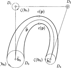
Figure 3.9 Tolerance region of a Bézier curve with disks Di as tolerance regions for the control points.
Generalizations to arbitrary convex tolerance regions for the input points are discussed in [35],[85],[108]. There, other problems of geometric tolerancing and error propagation in geometric constructions are addressed as well. Various applications of Laguerre geometry and the cyclographic mapping appear in connection with toleranced circles or spheres.
Further investigations of geometric tolerancing in the plane could make use of very recent work by Farouki et al. [29],[30]. It concerns the geometry of sets in the plane, which can be represented in a simple way using complex numbers. Complex numbers are known as elegant tool for certain geometric investigations, for example in planar kinematics and Möbius geometry [102].
3.2.4 The medial axis transform in a sphere geometric approach
Let D denote a planar domain with boundary σD. The (ordinary, trimmed) medial axis ![]() is the locus of centers of maximal disks that are contained in D; see chapter 19 for a detailed discussion on this topic.
is the locus of centers of maximal disks that are contained in D; see chapter 19 for a detailed discussion on this topic.
The construction of ![]() allows a Laguerre geometric interpretation, after embedding the plane of D into
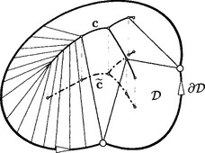
allows a Laguerre geometric interpretation, after embedding the plane of D into ![]() 3 as Π: x3 = 0: We search for a space curve c whose cyclographic image ζ(c) is ∂D (see Figure 3.10 and [37],[87]). Let ∂D be oriented such that its curve normals are pointing outside. Then ∂D defines a γ-developable Γ passing through σD, i.e., a developable surface whose generators are γ-lines. The set c of all self-intersections of Γ is called the (untrimmed) medial axis transform of D. The orthogonal projection of c onto Π gives the (untrimmed or complete) medial axis
3 as Π: x3 = 0: We search for a space curve c whose cyclographic image ζ(c) is ∂D (see Figure 3.10 and [37],[87]). Let ∂D be oriented such that its curve normals are pointing outside. Then ∂D defines a γ-developable Γ passing through σD, i.e., a developable surface whose generators are γ-lines. The set c of all self-intersections of Γ is called the (untrimmed) medial axis transform of D. The orthogonal projection of c onto Π gives the (untrimmed or complete) medial axis ![]() . It is the locus of (oriented) circles that touch the boundary ∂D in at least two points, but are — because of the lack of trimming—not neccesarily contained in D.
. It is the locus of (oriented) circles that touch the boundary ∂D in at least two points, but are — because of the lack of trimming—not neccesarily contained in D.
The above construction of the (untrimmed) medial axis transform allows the computation via surface/surface intersection algorithms, which are discussed in chapter 25. Those parts of the intersection curve which belong to the trimmed medial axis can be easily detected by a visibility algorithm: The interesting part of c lies in the upper half space x3 > 0 of ![]() 3. If the surface Γ is thought as opaque, exactly the part of c which is visible from below corresponds to the trimmed medial axis.
3. If the surface Γ is thought as opaque, exactly the part of c which is visible from below corresponds to the trimmed medial axis.
The medial axis transform c uniquely determines the boundary of the domain D via the cyclographic image of c. In general, σD will not be rational. The most general class of curves c whose cyclographic images are rational are so-called Minkowski Pythagorean-hodograph (MPH) curves (see Choi et al. [16] and Moon [66]). For a more detailed treatment see Chapters 17 and 19.
3.2.5 Canal surfaces (in Laguerre and Möbius geometry)
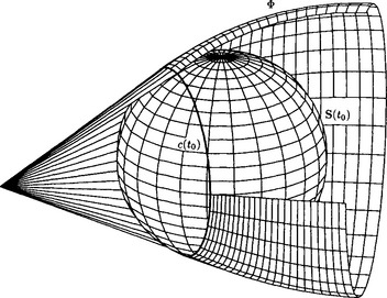
A canal surface Φ in Euclidean 3-space E3 is defined as envelope surface of a one parameter family of spheres S(t) = (m(t), r(t)) (see Figure 3.11).
The sphere family may be written in dependency on the real parameter t,
To compute the envelope, one has to form the derivative with respect to t, which is a plane
For a parameter t0 with ![]() , the intersecting circle c(t0) = S(t0) ∩
, the intersecting circle c(t0) = S(t0) ∩ ![]() (t0) is called characteristic circle. Along c(t0) the sphere S(t0) is in smooth contact with the canal surface Φ.
(t0) is called characteristic circle. Along c(t0) the sphere S(t0) is in smooth contact with the canal surface Φ.
For a Laguerre-geometric interpretation of Φ we allow oriented radii r(t) of S(t). A canal surface can be obtained as cyclographic image ζ(p(t)) of the curve p(t) = (m(t), r(t)) ∈ ![]() 4, as described in section 3.2.1. If the tangent line
4, as described in section 3.2.1. If the tangent line ![]() to parameter t0 encloses an angle α ≥ Π/4 with the 3-space Π: x4 = 0, the characteristic circle on the corresponding (oriented) sphere S(t0) is real.
to parameter t0 encloses an angle α ≥ Π/4 with the 3-space Π: x4 = 0, the characteristic circle on the corresponding (oriented) sphere S(t0) is real.
Besides the Laguerre geometric interpretation of a canal surface as cyclographic image of a space curve, canal surfaces can also be seen from a Möbius geometric point of view: A real canal surface in ![]() 3 is determined by a curve c
3 is determined by a curve c ![]() (t) in the quadric model P4 whose tangent lines do not intersect the Möbius quadric ∑ (a tangent line intersecting ∑ can be shown to be equivalent to the corresponding characteristic circle not being real).
(t) in the quadric model P4 whose tangent lines do not intersect the Möbius quadric ∑ (a tangent line intersecting ∑ can be shown to be equivalent to the corresponding characteristic circle not being real).
We see that from the standpoint of both Laguerre and Möbius geometry, canal surfaces have a representation as curves in 4-dimensional space. Partially by using sphere geometric methods, it could be proved that rationality of these curves implies the existence of a rational parameterization of the corresponding canal surfaces [51],[71],[73],[74].
Thus, these curve models are well suited for design. Approximation and interpolation schemes for curves can be used for approximation or blending schemes with canal surfaces [63],[70],[87]; see also section 3.4.1.
A very important family of canal surfaces in CAGD are the Dupin cyclides, see chapter 23. In the cyclographic model of Laguerre geometry they are represented as pseudo-Euclidean circles in ![]() 4, i.e., conics that are planar intersections of γ-hypercones. Thus, well-known biarc interpolation schemes can be used to construct G1-canal surfaces composed of smoothly joined cyclide patches [87]. Furthermore, the Bézier control points of Dupin cyclide patches and the connection of cyclide patches along cubic or quartic curves can be discussed based on Laguerre geometry [50],[64],[72].
4, i.e., conics that are planar intersections of γ-hypercones. Thus, well-known biarc interpolation schemes can be used to construct G1-canal surfaces composed of smoothly joined cyclide patches [87]. Furthermore, the Bézier control points of Dupin cyclide patches and the connection of cyclide patches along cubic or quartic curves can be discussed based on Laguerre geometry [50],[64],[72].
3.2.6 Rational curves and surfaces with rational offsets
An offset cd(t) of a given planar curve c(t) lies in constant normal distance d to c. With help of a field of unit normal vectors n(t) of c(t), the two ‘one-sided’ offsets are cd(t) = c(t) + dn(t), where d may have a positive or negative sign. Analogously, we define the offsets of a surface in ![]() 3. Offsets possess important applications, for example in NC machining. For the rich literature on this topic, we refer to the survey by T. Maekawa [59].
3. Offsets possess important applications, for example in NC machining. For the rich literature on this topic, we refer to the survey by T. Maekawa [59].
Given a rationally parameterized curve c(t), the unit normal vectors are in general not rational in t, and thus the offsets of rational curves are in general not rational. However, CAD systems require piecewise rational representations and thus offsets need to be approximated. Another possibility is to use only those rational curves or surfaces which do have rational offsets.
chapter 17 is exclusively devoted to polynomial and rational Pythagorean-hodograph (PH) curves and gives an extensive overview of the literature on this topic. In the plane, PH curves are polynomial curves whose offsets are rational curves. They can be defined as those polynomial curves whose hodograph (x′(t), y′(t)) satisfies the Pythagorean equation x′2(t) + y′2(t) = σ2(t) for some polynomial σ(t). This property motivates the name ‘PH curve’ and is equivalent to the existence of a polynomial arc length function.
Here we will just skim the surface of the theory of rational curves with rational offsets, also referred to as rational PH curves. In particular we will stress the close relation of rational PH curves to certain rational developable surfaces via the cyclographic mapping introduced in section 3.2.1.
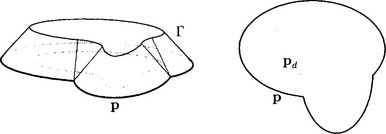
As outlined in section 3.2.4, an oriented planar curve p ⊂ Π defines a γ-developable surface Γ passing through p. The planar intersections of Γ with horizontal planes x3 = d, projected orthogonally onto the plane Π, give the (one-sided) offset pd to signed distanced (see Figure 3.12).
Keeping this property in mind, one can classify rational PH curves as planar horizontal intersection curves of rational γ-developables Γ. In general, Γ is the tangent surface of a spatial curve c of constant slope γ = Π/4, i.e., all of the curve tangents are γ-lines. Obviously Γ is rational if and only if the curve c is. Since c has constant slope Π/4, its third coordinate function x3(t) equals, up to an additive constant, the total arc length of the top projection c′(t) = (x1(t), x2(t), 0). All the offsets of the PH curves share a common evolute, which is the top projection c′ of c onto Π. This can be used to obtain the following characterization: Rational PH curves are exactly the involutes of rational curves with rational arc length function [78].
Rational γ-developables are easily described in their dual form, and the same holds for rational PH curves. Explicit representations are found in [78].
The description of rational PH curves gets even simpler when one uses the dual Bezier control structure as described in section 3.1.3. A rational PH curve and its offsets have control and frame lines that are related to each other and to a certain dual rational representation of a circle segment by parallel translation. For a detailed treatment of this property, see [78],[79],[100]. In [79], special rational PH curves, namely cyclographic images of certain conics (studied first by W. Blaschke [7]), have been used to design curvature continuous rational curves with rational offsets.
Whereas the approach to PH curves taken by Farouki and Sakkalis [31] does not have a generalization to surfaces, the dual and Laguerre geometric approach to rational PH curves extend to surfaces [78],[74],[101]. These Pythagorean-normal (PN) surfaces possess rational offset surfaces. A remarkably simple characterization of rational curves and surfaces with rational offsets is within the isotropic model of Laguerre geometry. There, these curves (surfaces), viewed as envelopes of their oriented tangents (tangent planes), appear as arbitrary rational curves or surfaces. The change between two models of Laguerre geometry transforms an arbitrary rational curve or surface into a rational PH curve or PN surface, respectively [72],[74]. The suitability of Laguerre geometry for studying curves and their offsets is not surprising in view of the fact that the mapping from a curve/surface to an offset of it can be performed with a special Laguerre transformation.
Special polynomial surfaces with rational offsets have been applied to surface designby Jüttler and Sampoli [46]. The family of PN surfaces includes the following classes of rational surfaces: Regular quadrics [58],[74], canal surfaces with rational spine curve m(t) and rational radius function r(t) [51],[71],[73],[74], and skew rational ruled surfaces [84]. Using Laguerre and Möbius geometry, PN surfaces which generalize Dupin cyclides in the sense that they also possess rational principal curvature lines, have been studied by Pottmann and Wagner [92].
Quadrics, canal surfaces as well as skew ruled surfaces are enveloped by a one parameter set of cones of revolution. Cones of revolution are the cyclographic images of lines in ![]() 4 which enclose an angle smaller than Π/4 to the embedded 3-space Π. Using this property it is possible to show that any rational one parameter family of cones of revolution envelopes a PN surface [71]. M. Peternell [71] extended this result to other families of quadrics which possess a rationally parametrizable envelope.
4 which enclose an angle smaller than Π/4 to the embedded 3-space Π. Using this property it is possible to show that any rational one parameter family of cones of revolution envelopes a PN surface [71]. M. Peternell [71] extended this result to other families of quadrics which possess a rationally parametrizable envelope.
Offsets of surfaces are of importance in NC milling [61] when using a spherical milling tool. As the milling tool is touching the surface the midpoint of the ball must be located on the offset surface to a distance equaling the radius of the cutting tool. Natural generalizations of offset surfaces occur if the milling tool — which is rotating around its axis — is not a spherical one but a general rotational surface [61],[81]. The special case of a cylindrical milling tool (flat end mill) yields circular offset surfaces. A geometric interpretation via Galilei sphere geometry can be found in [107].
3.3 LINE GEOMETRY
Line geometry investigates the set of lines in three-space. There is rich literature on this classical topic of geometry including several monographs [25],[36],[38],[68],[94],[112],[116]. Line geometry possesses a close relation to spatial kinematics [11],[45],[103],[106],[112], see also chapter 29. Line geometry enters problems in geometric computing in various ways. A detailed account of the use of line geometry in geometric modeling and related areas is given in a monograph by Pottmann and Wallner [94]. In the following, we briefly outline just a few basic principles and typical applications.
3.3.1 Basics of line geometry
A straight line L in Euclidean 3-space E3 can be determined by a point p ∈ L and a normalized direction vector l of L, i.e. ||l|| = 1. To obtain coordinates for L, one forms the moment vector Ī:= p Λ l, with respect to the origin. Ī is independent of the choice of p ∈ L. The six coordinates (l,Ī) with
are called normalized Plücker coordinates of L. With normalized l, the distance of the origin o to the line L simply equals ||Ī||.
However, one may give up the normalization condition and interpret (l1 …, l6)![]() as a point in a 5-dimensional projective space P5. Note that l and Ī are orthogonal, thus
as a point in a 5-dimensional projective space P5. Note that l and Ī are orthogonal, thus
holds. Equation (3.12) is the so-called Plücker identity and describes a hyperquadric ![]() in P5, the Klein quadric.
in P5, the Klein quadric. ![]() is a four-dimensional manifold and each of its points L
is a four-dimensional manifold and each of its points L ![]() = (l, Ī)
= (l, Ī)![]() with l ˙ Ī = 0 describes a line L in the projective extension P3 of Euclidean 3-space E3. Lines L at infinity are characterized by l = o.
with l ˙ Ī = 0 describes a line L in the projective extension P3 of Euclidean 3-space E3. Lines L at infinity are characterized by l = o.
Summarizing, the use of homogeneous Plücker coordinates for lines in P3 and their interpretation as points in P5 results in a point model for line space, which is called Klein model. Lines in P3 correspond to points on the Klein quadric ![]() ⊂ P5.
⊂ P5.
A line L may be spanned by two points x ![]() and y
and y ![]() , possibly at infinity. In the following it will turn out convenient to write x = (x0, x) with x0 ∈
, possibly at infinity. In the following it will turn out convenient to write x = (x0, x) with x0 ∈ ![]() and x ∈
and x ∈ ![]() 3. Note that here x does not denote the affine coordinates of x
3. Note that here x does not denote the affine coordinates of x ![]() , but a scalar multiple of them. The homogeneous Plücker coordinates of L are found as
, but a scalar multiple of them. The homogeneous Plücker coordinates of L are found as
Basic geometric relations with lines, like intersecting a line with a plane or connecting a line with a point result in simple linear equations in homogeneous point, line, and plane coordinates. These formulae can be found in each book on line geometry. As an example we will just mention the intersection condition of two lines ![]() and
and ![]() ,
,
It characterizes G, H as two conjugate points with respect to the Klein quadric ![]() , i.e., they are lying in each others polar hyperplane with respect to
, i.e., they are lying in each others polar hyperplane with respect to ![]() .
.
3.3.2 Linear complexes in kinematics and reverse engineering
A 3-parameter set of lines L = (1,Ī)![]() satisfying a linear equation in Plücker coordinates,
satisfying a linear equation in Plücker coordinates,
is called a linear line complex or linear complex C. With ![]() we can rewrite (3.14) as
we can rewrite (3.14) as ![]() , where c ˙
, where c ˙ ![]() not neccessarily equals 0, i.e., C
not neccessarily equals 0, i.e., C![]() does not need to describe a line.
does not need to describe a line.
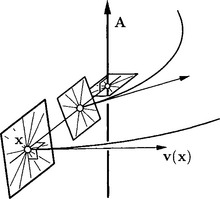
The connection of linear complexes to kinematics is given as follows. Let us consider a continuous helical motion, that is composed of a continuous rotation around a line A and a continuous translation parallel to A. In an appropriate coordinate system we have
In an arbitrary coordinate system the (time independent) velocity vector field for such a motion is v(x) = ![]() + c Λ x with constant vectors c,
+ c Λ x with constant vectors c, ![]() , see Bottema and Roth [11].
, see Bottema and Roth [11].
Lines through points x normal to v(x) are normal to the trajectory of x and are called path normals, see Figure 3.13. It is easy to show that the path normals L of a helical motion satisfy ![]() ˙ l + c ˙ ī, thus lie in a linear complex.
˙ l + c ˙ ī, thus lie in a linear complex.
If the pitch p in (3.15) equals zero, we obtain a pure rotation. The vectors c, ![]() then will fulfill c ˙
then will fulfill c ˙ ![]() = 0 and determine the rotational axis A which is intersected by all of the motion’s path normals.
= 0 and determine the rotational axis A which is intersected by all of the motion’s path normals.
Linear complexes as simple ‘linear manifolds’ of lines play an important role in various applications. Subsequently, we will address two of them.
The first application is in reverse engineering of geometric objects (see chapter 26), where we consider the following problem: Given a cloud of measurement points from a surface, decide whether this cloud can be fitted well by a helical or rotational surface, and if so, construct such an approximating surface.
A helical surface is swept out by a curve which undergoes a continuous helical motion. For vanishing pitch p of the motion, we obtain a rotational surface. It is easy to see that all surface normals of a helical surface lie in the path normal complex of the generating helical motion. Conversely, it can be shown that a surface all whose normals lie in a linear complex must be be a helical surface, a rotational surface (p = 0) or a general cylinder surface (limit case with p = ∞).
Thus, the above reconstruction problem can be solved as follows. We estimate surface normals at the given data points. Those should lie, up to some small deviations, in a linear complex. After defining the deviation of a line L from a linear complex C this leads to an approximation problem in line space. It amounts to a general eigenvalue problem, whose eigenvalues also tell us about the presence of special cases (plane, sphere, right circular cylinder) [89],[90].
Another application concerns the stability of a six-legged parallel manipulator. There, a moving system ∑ is linked to a fixed base system ∑0 via six legs, realized as hydraulic cylinders, which are attached to both systems via spherical joints. If these six legs (axes of the hydraulic cylinders) lie nearly in a linear complex, the position of the platform ∑ gets instable [65],[89]. Thus, the determination of instable positions amounts to fitting a linear complex to the axes of the parallel manipulator.
3.3.3 Ruled surfaces
Ruled surfaces are generated by moving a straight line in 3-space. In the Klein model of line space they appear as curves on the Klein quadric ![]() [25]. The point model may be advantageous, because for some applications it is easier to deal with curves, even in projective 5-space, than working with ruled surfaces. Approximation and Hermite interpolation algorithms for ruled surfaces amount to corresponding algorithms for curves on the quadric
[25]. The point model may be advantageous, because for some applications it is easier to deal with curves, even in projective 5-space, than working with ruled surfaces. Approximation and Hermite interpolation algorithms for ruled surfaces amount to corresponding algorithms for curves on the quadric ![]() (see chapter 31 on quadrics, and [76],[94]).
(see chapter 31 on quadrics, and [76],[94]).
For example, Peternell et al. [76] have formulated algorithms for the approximation of ruled surfaces by low degree algebraic ruled surfaces (ruled quadrics, cubic and quintic ruled surfaces) and have presented a G1 Hermite interpolation scheme resulting in piecewise quadratic ruled surfaces.
Line geometry applied to CAD has also been considered by Ravani et al. [33],[34],[96],[104], where line geometric counterparts to subdivision algorithms for curves and surfaces, like de Casteljau’s algorithm, are developed.
3.3.4 Other applications of line geometry in geometric computing
Line geometry is a basic entity in the formulation of the so-called generalized stereographic projection σ, also known as Hopf mapping. It maps points in projective 3-space P3 onto points of the Euclidean sphere S2. The preimage of a point on S2 under this mapping σ is a straight line in P3. All fibers of σ form a so-called elliptic linear line congruence in P3. It may be seen as intersection of two appropriate linear complexes, and the Klein image of the line congruence is an oval quadric in ![]() . Dietz, Hoschek, and Jüttler [22] have shown that the mapping σ is well-suited to construct rational curve and surface patches on the sphere. Applying a projective mapping, one can work on other oval quadrics as well. It can also be used for the definition of a B-spline like intrinsic control structure for NURBS curves on the sphere [80]. There are similar mappings for ruled quadrics and singular quadrics [21], whose fibers are line congruences (intersections of two linear complexes). Such mappings are useful for the design of curves and surface patches on quadrics (see also chapter 31), and they can also be used to construct rational blending surfaces between quadrics [109].
. Dietz, Hoschek, and Jüttler [22] have shown that the mapping σ is well-suited to construct rational curve and surface patches on the sphere. Applying a projective mapping, one can work on other oval quadrics as well. It can also be used for the definition of a B-spline like intrinsic control structure for NURBS curves on the sphere [80]. There are similar mappings for ruled quadrics and singular quadrics [21], whose fibers are line congruences (intersections of two linear complexes). Such mappings are useful for the design of curves and surface patches on quadrics (see also chapter 31), and they can also be used to construct rational blending surfaces between quadrics [109].
A generalization of the mapping σ to the construction of rational curves and surface patches on Dupin cyclides has been studied by C. Mäurer [62].
Line geometry also appears in manufacturing, such as sculptured surface machining [91],[111] and wire cut EDM [96]. For further applications and detailed discussions, we refer the reader to Pottmann and Wallner [94].
3.4 APPROXIMATION IN SPACES OF GEOMETRIC OBJECTS
For different geometric objects in E3 there exist point models: Oriented spheres can be represented as points in the cyclographic model, see section 3.2.1. Planes are represented as points in dual projective space, see section 3.1.3. Lines are represented as points on a hyperquadric ![]() in P5, see section 3.3.1.
in P5, see section 3.3.1.
Approximation schemes in the spaces of spheres, planes, lines or other geometric objects require a point model and an appropriate distance defined for these geometric objects. After mapping the point model to an affine space one will define an appropriate Euclidean metric, which is motivated by a deviation measure between two objects. Here we will briefly mention the deviation measures in the spaces of spheres, planes and lines, and resulting approximation schemes for canal surfaces (section 3.4.1), developable surfaces (section 3.4.2) and ruled surfaces (section 3.4.3). For details, see Pottmann and Peternell [75],[88].
3.4.1 Approximation in the space of spheres
In the cyclographic model of 3-dimensional Euclidean Laguerre geometry, oriented spheres S are seen as points ζ−1(S) = (m1, m2, m3, r). The distance of two oriented spheres A: (a1,…,a4) and B: (b1,…,b4) can be defined via the canonical Euclidean distance of their image points in ![]() 4,
4,
A geometric interpretation of d(A, B) can be found in [88]. With help of the above metric in ![]() 4 one can use standard Bézier and B-spline techniques for curve design in
4 one can use standard Bézier and B-spline techniques for curve design in ![]() 4, and one obtains rational canal surfaces as the cyclographic images of the designed curves. Here, the geometric continuity (chapter 8) is preserved: a Gk curve gives rise to a Gk canal surface.
4, and one obtains rational canal surfaces as the cyclographic images of the designed curves. Here, the geometric continuity (chapter 8) is preserved: a Gk curve gives rise to a Gk canal surface.
3.4.2 Approximation in the space of planes
The set of planes in P3 is a 3-dimensional projective space itself. The homogeneous coordinates U = (u0, u1, u2, u3) of a plane U are the coefficients of the plane’s equation u0+u1x+u2y+u3z = 0, see section 3.1.3. If we work in Euclidean 3-space and restrict ourselves to planes which are not parallel to the z-axis of a Cartesian system, i.e., u3 ≠ 0, we can normalize the plane coordinates to U = (u0, u1, u2, − 1) and obtain affine coordinates (u0, u1, u2) ∈ A3 of U. Note that one may choose an appropriate coordinate system to avoid that planes of interest are parallel to the z-axis.
The distance of two planes A, B within some region of interest may be defined by
which equals the squared z-differences of A and B, integrated over a fixed domain Γ of interest in the xy-plane, see Figure 3.14. The such defined dΓ is a positive definite quadratic form in ai - bi, whose constant coefficients are certain integrals that can be easily computed. Thus, dΓ introduces a Euclidean metric in affine 3-space A3.
One parameter sets of planes envelop developable surfaces which correspond to curves in A3. Again, standard Bézier and B-spline approximation techniques can be used, e.g., to approximate a discrete set of tangent planes with a NURBS developable surface, see Figure 3.14. Details and the important task of controlling the singularities are discussed in [42],[93],[94].
3.4.3 Approximation in line space
Consider two parallel planes Π0, Π1 in ![]() 3 and the set
3 and the set ![]() of all lines which are not parallel to them. Then intersection of any line in
of all lines which are not parallel to them. Then intersection of any line in ![]() with Π0, Π1 gives a pair x0 = (l1, l2), x1 = (l3, l4) of points, which may be considered as point L = (l1,l2,l3, l4) in real affine 4-space
with Π0, Π1 gives a pair x0 = (l1, l2), x1 = (l3, l4) of points, which may be considered as point L = (l1,l2,l3, l4) in real affine 4-space ![]() 4. This mapping from
4. This mapping from ![]() onto
onto ![]() 4 can be interpreted as stereographic projection of the Klein quadric
4 can be interpreted as stereographic projection of the Klein quadric ![]() .
.
The affine image space can be equipped with the Euclidean metric
It corresponds to a distance of the two lines A, B within the parallel strip bounded by planes Π0, Π1 (region of interest). It is obtained by integrating the squared distances between the lines, measured horizontally, see Figure 3.15.
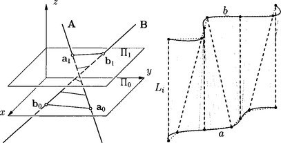
Figure 3.15 Left: Distance between lines measured horizontally; Right: Ruled surface approximating seven (dashed) lines Li.
The Euclidean metric d(A, B) defined above is useful for solving various approximation problems in line space [14],[94]. It has also been used to compute the approximation of given lines Li by a ruled surface in Figure 3.15, see [88] for details.
3.5 NON-EUCLIDEAN GEOMETRIES
3.5.1 Hyperbolic geometry and geometric topology
Although we are usually designing in Euclidean space, there are various examples for applications of non-Euclidean geometries in geometric modeling.
A remarkable application is the following. Consider the hyperbolic plane H2, a model of which can be realized as follows. Take a circular disk with bounding circle u. The points in the open disk are the points of the hyperbolic plane. Collinear points in hyperbolic geometry lie on circles (or straight lines) which intersect u orthogonally. Such hyperbolic straight line segments are seen in Figure 3.16, left. Hyperbolic congruences are seen in this special model as Möbius transformations which preserve u as a whole.
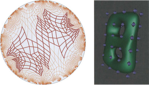
Figure 3.16 Tesselation of the hyperbolic plane (left); a function which is invariant under the associated discrete group is suitable for parametrizing a closed orientable surface of genus two (right).
There are other models of the hyperbolic plane, which are more appropriate for computations. One of these is the projective model, where points and lines appear as points and line segments inside a circle u and congruence transformations are given by projective maps which preserve u as a whole.
In the hyperbolic plane, there exist remarkable discrete groups G of congruences. They possess a domain F bounded by 4g-gon (g being an integer > 2) as fundamental domain. This means that application of the elements of the group G to F generates a tiling of the hyperbolic plane. Figure 3.16, left, shows such a tiling for g = 2. It illustrates a slightly more complicated fundamental domain, which is, however, equivalent to an octogon as the group in the sense that its value f(x) at a point x ∈ H2 and at all images of x under the elements of G are the same. Then, three such functions, evaluated at the fundamental domain F, may be seen as coordinate functions of a parametric surface in 3-space. It is well-known that this surface is a closed orientable surface of genus g and that all closed orientable surfaces of genus g > 2 may be obtained via hyperbolic geometry in this way [95],[115].
This hyperbolic approach to the design of closed surfaces of arbitrary genus and smoothness has first been taken by Ferguson and Rockwood [32]. [110] have further investigated this direction and shown, for example, how to design piecewise rational surfaces with arbitrarily high geometric continuity. Although theoretically very elegant, the practical use for complicated shapes seems to be limited. Most likely, subdivision based schemes will be preferred for applications.
3.5.2 Elliptic geometry and kinematics
The intrinsic geometry of the n-dimensional Euclidean sphere Sn ⊂ En+1, with identification of antipodal points, is called elliptic geometry. Three-dimensional elliptic geometry is very closely related to spherical kinematics and has important applications in the design and analysis of motions on the sphere and in Euclidean 3-space [69]. This relation as well as applications in computer animation and robot motion planning are discussed in chapter 29.
3.5.3 Isotropic geometry and analysis of functions and images
In order to visualize the function f: D ⊂ ![]() 2 →
2 → ![]() , defined on a region D of the Euclidean plane E2 =
, defined on a region D of the Euclidean plane E2 = ![]() 2, we usually embed this plane as (x1, x2)-plane into 3-space
2, we usually embed this plane as (x1, x2)-plane into 3-space ![]() 3 and consider the graph surface Γ(f):= {(x1, x2, f(x1, x2)) ∈
3 and consider the graph surface Γ(f):= {(x1, x2, f(x1, x2)) ∈ ![]() 3: (x1, x2) ∈ D}. This natural procedure is sometimes followed by the seemingly natural assumption to interpret
3: (x1, x2) ∈ D}. This natural procedure is sometimes followed by the seemingly natural assumption to interpret ![]() 3 as Euclidean space. However, it is much more appropriate for many applications to introduce a so-space. However, it is much more appropriate for many applications to introduce a so-called isotropic metric in
3 as Euclidean space. However, it is much more appropriate for many applications to introduce a so-space. However, it is much more appropriate for many applications to introduce a so-called isotropic metric in ![]() 3. In isotropic geometry, one investigates properties which are invariant under the following group of affine mappings,
3. In isotropic geometry, one investigates properties which are invariant under the following group of affine mappings,
Like the Euclidean motion group in ![]() 3, this group of so-called isotropic motions depends on six real parameters Φ, α1,…, α5. As seen from the first two equations in (3.17), an isotropic motion appears as Euclidean motion in the projection onto the plane x3 = 0. A careful study of isotropic geometry in two and three dimensions is found in the monographs by H. Sachs [97],[98].
3, this group of so-called isotropic motions depends on six real parameters Φ, α1,…, α5. As seen from the first two equations in (3.17), an isotropic motion appears as Euclidean motion in the projection onto the plane x3 = 0. A careful study of isotropic geometry in two and three dimensions is found in the monographs by H. Sachs [97],[98].
The application to the analysis and visualization of functions defined on Euclidean spaces is studied in [86]. For example, the standard thin plate spline functional in two dimensions,
has a purely geometric interpretation for the graph surface of f within isotropic geometry. It is the surface integral over the sum of squares of isotropic principal curvatures x1, x2,
The use of isotropic geometry has been extended to functions defined on surfaces (chapter 9) rather than flat Euclidean spaces [86]. Currently, it is investigated by J. Koenderink for understanding images of surfaces along the lines described in [49].
Isotropic geometry also appears in the context of Laguerre geometry, namely in the so-called isotropic model. For example, the oriented tangent planes of a right circular cone appear as an isotropic circle in the isotropic model. This is in general a conic, whose projection onto x3 = 0 is a Euclidean circle. Smooth spline curves formed by such conic segments could be called “isotropic arc splines”. Their construction is completely analogous to arc splines in Euclidean 3-space. The transformation back to the standard model of Laguerre geometry gives developable surfaces, which consist of smoothly joined pieces of right circular cones [55]. Geometric computing with these cone spline surfaces rather than general developables has a variety of advantages: The computation of bending sequences and the planar development can be performed in an elementary way. The degree, namely two for both the implicit and parametric representation of the segments, is the lowest possible for generating smooth surfaces, and the offsets are of the same type [54],[56].
1. Albrecht, G. A note on Farin points for rational triangular Bézier patches. Computer Aided Geometric Design. 1995;12:507–512.
2. Albrecht, G. Rational Triangular Bézier Surfaces – Theory and Applications. New York: Shaker Verlag; 1999.
3. Aumann, G. Interpolation with developable Bezier patches. Computer Aided Geometric Design. 1991;8:409–420.
4. Amar, M. Ben, Pomeau, Y., Crumpled paper. Proc. Royal Soc. London, 1997;A453:729–755.
5. Benz, W. Geometrische Transformationen. Aachen: BI-Wiss. Verlag; 1992.
6. Bertini, E. Einführung in die projektive Geometrie mehrdimensionaler Räume, 2nd ed. Mannheim: Seidel & Sohn; 1924.
7. Blaschke, W. Untersuchungen über die Geometrie der Speere in der Euklidischen Ebene. Monatshefte für Mathematik und Physik. 1910;21:3–60.
8. Blaschke, W. Vorlesungenüber Differentialeometrie, Vol. III. Springer: Wien, 1929.
9. Bodduluri, R.M.C., Ravani, B. Design of developable surfaces using duality between plane and point geometries. Computer-Aided Design. 1993;25:621–632.
10. Bol, G., Projektive. Differentialeometrie I, II, III. 1950, 1954. Vandenhoeck & Ruprecht: Berlin, 1967.
11. Bottema, O., Roth, B. Theoretical Kinematics. Göttingen: Dover Publ; 1990.
12. Cecil, T.E. Lie Sphere Geometry. New York: Springer; 1992.
13. Chalfant, J., Maekawa, T. Design for manufacturing using B-spline developable surfaces. J. Ship Research. 1998;42:207–215.
14. Chen, H.Y., Pottmann, H. Approximation by ruled surfaces. J. Comput. Applied Math. 1999;102:143–156.
15. Chen, H.Y., Lee, I.K., Leopoldseder, S., Pottmann, H., Randrup, T., Wallner, J. On surface approximation using developable surfaces. Graphical Models and Image Processing. 1999;61:110–124.
16. Choi, H.I., Han, C.Y., Moon, H.R., Roh, K.H., Wee, N.S. Medial axis transform and offset curves by Minkowski Pythagorean hodograph curves. Computer-Aided Design. 1999;31:59–72.
17. Coolidge, J.L. A Treatise on the Circle and the Sphere. Berlin, Heidelberg, New York: Clarendon Press; 1916.
18. Degen, W.L.F. Some remarks on Bézier curves. Computer Aided Geometric Design. 1988;5:259–268.
19. Degen, W.L.F., Projektive differential geometrie. Giering O., Hoschek J., eds., eds. Geometrie und ihre Anwendungen Hanser, München. 1994:319–374.
20. Degen, W.L.F. The types of triangular Bézier surfaces. In: Mullineux G., ed. The Mathematics of Surfaces VI. Oxford: Clarendon Press; 1996:153–170.
21. Dietz, R. Rationale Bézier-Kurven und Bézier-Flächenstücke auf Quadriken. Diss, TH Darmstadt. 1995.
22. Dietz, R., Hoschek, J., Jüttler, B. An algebraic approach to curves and surfaces on the sphere and on other quadrics. Computer Aided Geometric Design. 1993;10:211–229.
23. Edelsbrunner, H. Deformable smooth surface design. Discrete Comput. Geom. 1999;21:87–115.
24. Edelsbruner, H., Bio-Geometric Modeling. Lecture Notes. Duke University: Oxford, 2001.
25. Edge, W.L. The Theory of Ruled Surfaces. Cambridge University Press; 1931.
26. Farin, G. Algorithms for rational Bézier curves. Computer-Aided Design. 1983;15:73–77.
27. Farin, G. NURBS for Rational Curve and Surface Design. Cambridge, UK: AK Peters; 1994.
28. Farin, G. Curves and Surfaces for Computer Aided Geometric Design, Fourth ed. Boston: Academic Press; 1997.
29. Farouki, R.T., Moon, H.P., Ravani, B. Algorithms for Minkowski products and implicitly defined complex sets. Advances in Comp. Math. 2000;13:199–229.
30. Farouki, R.T., Moon, H.P., Ravani, B. Minkowski geometric algebra of complex sets. Geometriae Dedicata. 2001;85:283–315.
31. Farouki, R.T., Sakkalis, T. Pythagorean hodographs. IBM J. Res. Develop. 1990;34:736–752.
32. Ferguson, H., Rockwood, A. Multiperiodic functions for surface design. Computer Aided Geometric Design. 1993;10:315–328.
33. Ge, Q.J., Ravani, B. On representation and interpolation of line segments for computer aided geometric design. ASME Design Automation Conf. 1994;96(1):191–198.
34. Ge, Q.J., Ravani, B. Geometric design of rational Bézier line congruences and ruled surfaces using line geometry. Computing. 1998;13:101–120.
35. Hinze, C.U. A Contribution to Optimal Tolerancing in 2-Dimensional Computer Aided Design. Dissertation, Kepler University Linz. 1994.
36. Hlavaty, V. Differential Line Geometry. San Diego: P. Nordhoff Ltd; 1953.
37. Berlin Hoffmann, C. Computer vision, descriptive geometry and classical mechanics. In: Falcidieno B., et al, eds. Computer Graphics and Mathematics. Groningen: Springer Verlag; 1992:229–243.
38. Hoschek, J. Liniengeometrie. Bibliograph. Institut; 1971.
39. Hoschek, J. Dual Bézier curves and surfaces. In: Barnhill R.E., Boehm W., eds. Surfaces in Computer Aided Geometric Design. Zürich: North Holland; 1983:147–156.
40. Hoschek, J. Detecting regions with undesirable curvature. Computer Aided Geometric Design. 1984;1:183–192.
41. Hoschek, J., Lasser, D. Fundamentals of Computer Aided Geometric Design. A.K. Peters; 1993.
42. Hoschek, J., Pottmann, H. Interpolation and approximation with developable B-spline surfaces. In: Daehlen M., Lyche T., Schumaker L.L., eds. Mathematical Methods for Curves and Surfaces. Wellesley, MA: Vanderbilt University Press; 1995:255–264.
43. Hoschek, J., Schneider, M. Interpolation and approximation with developable surfaces. In: Le Méhauté A., Rabut C., Schumaker L.L., eds. Curves and Surfaces with Applications in CAGD. Nashville (TN): Vanderbilt University Press; 1997:185–202.
44. Hoschek, J., Schwanecke, U. Interpolation and approximation with ruled surfaces. In: Cripps R., ed. The Mathematics of Surfaces VIII. Nashville (TN): Information Geometers; 1998:213–231.
45. Hunt, K.H. Kinematic Geometry of Mechanisms. Winchester: Clarendon Press; 1978.
46. Jüttler, B., Sampoli, M.L. Hermite interpolation by piecewise polynomial surfaces with rational offsets. Computer Aided Geometric Design. 17, 2000.
47. Jüttler, B., Wagner, M. Rational motion-based surface generation. Computer-Aided Design. 1999;31:203–213.
48. Kergosien, Y.L., Gotoda, H., Kunii, T.L. Bending and creasing virtual paper. IEEE Computer Graphics & Applications. 1994;14:40–48.
49. London Koenderink, J., van Doom, A., Kappers, A. Surfaces in the mind’s eye. In: Cipolla R., Martin R., eds. The Mathematics of Surfaces IX. Oxford: Springer; 2000:180–193.
50. Krasauskas, R., Mäurer, C. Studying cyclides with Laguerre geometry. Computer Aided Geometric Design. 2000;17:101–126.
51. Landsmann, G., Schicho, J., Winkler, F., Hillgarter, E. Symbolic parametrization of pipe and canal surfaces. In: Proceedings ISSAC-2000. ACM Press; 2000:194–200.
52. Lang, J., Röschel, O. Developable (1, n) Bézier surfaces. Computer Aided Geometric Design. 1992;9:291–298.
53. Leopoldseder, S. Cone Spline Surfaces and Spatial Arc Splines. Dissertation, Vienna Univ. of Technology. 1998.
54. Leopoldseder, S. Algorithm on cone spline surfaces and spatial osculating arc splines. Computer Aided Geometric Design. 2001;18:505–530.
55. to appear Leopoldseder, S., Cone spline surfaces and saptial arc splines – a sphere geometric approach. Advances in Computational Mathematics. 2001.
56. Leopoldseder, S., Pottmann, H. Approximation of developable surfaces with cone spline surfaces. Computer-Aided Design. 1998;30:571–582.
57. Lin, Q., Rokne, J. Disk Bézier curves. Computer Aided Geometric Design. 1998;15:721–737.
58. Lü, W. Rational parameterization of quadrics and their offsets. Computing. 1996;57:135–147.
59. Maekawa, T. An overview of offset curves and surfaces. Computer-Aided Design. 1999;31:165–173.
60. Maekawa, T., Chalfant, J.S. Computation of inflection lines and geodesies on developable surfaces. Math. Engineering in Industry. 1998;7:251–267.
61. Marciniak, K. Geometric Modelling for Numerically Controlled Machining. Oxford University Press; 1991.
62. Mäurer, C. Rationale Bézier-Kurven und Bézier-Flächenstücke auf Dupinschen Zykliden. Diss, Darmstadt. 1997.
63. Mäurer, C. Applications of sphere geometry in canal surface design. In: Laurent P.J., et al, eds. Curve and Surface Design: Saint Malo 1999. New York: Vanderbilt Univ. Press; 1999:267–276.
64. Mäurer, C., Krasauskas, R. Joining cyclide patches along quartic boundary curves. In: Dælen et al M., ed. Mathematical Methods for Curves and Surfaces II. Nashville: Vanderbilt Univ. Press; 1998:359–366.
65. Merlet, J.-P. Singular configurations of parallel manipulators and grassmann geometry. Int. J. Robotics Research. 1992;8:45–56.
66. Moon, H.P. Minkowski Pythagorean hodographs. Computer Aided Geometric Design. 1999;16:739–753.
67. Müller, E., Krames, J. Vorlesungen über Darstellende Geometrie II: Die Zyklographie. Nashville: Deuticke; 1929.
68. Miiller, E., Krames, J. Vorlesungen über Darstellende Geometrie III: Konstruktive Behandlung der Regelfächen. Leipzig, Wien: Deuticke; 1931.
69. Müller, H.R. Sphärische Kinematik. Leipzig, Wien: VEB Deutscher Verlag der Wissenschaften; 1962.
70. Paluszny, M., Boehm, W. General cyclides. Computer Aided Geometric Design. 1998;15:699–710.
71. Peternell, M. Rational Parameterizations for Envelopes of Quadric Families. Dissertation, Vienna Univ. of Technology. 1997.
72. Peternell, M., Pottmann, H. Designing rational surfaces with rational offsets. In: Fontanella F., Jetter K., Laurent P.J., eds. Advanced Topics in Multivariate Approximation. Berlin: World Scientific; 1996:275–286.
73. Peternell, M., Pottmann, H. Computing rational parametrizations of canal surfaces. J. Symbolic Computation. 1997;23:255–266.
74. Peternell, M., Pottmann, H. A Laguerre geometric approach to rational offsets. Computer Aided Geometric Design. 1998;15:223–249.
75. Peternell, M., Pottmann, H. Approximation in the space of planes – Applications to geometric modeling and reverse engineering. Technical Report 87, Institut für Geometrie, TU Wien. 2001.
76. Peternell, M., Pottmann, H., Ravani, B. On the computational geometry of ruled surfaces. Computer-Aided Design. 1999;31:17–32.
77. Piegl, L., Tiller, W. The NURBS Book. Springer-Verlag; 1995.
78. Pottmann, H. Rational curves and surfaces with rational offsets. Computer Aided Geometric Design. 1995;12:175–192.
79. Pottmann, H. Curve design with rational Pythagorean-hodograph curves. Advances in Comp. Math. 1995;3:147–170.
80. Pottmann, H. Studying NURBS curves and surfaces with classical geometry. In: Dæhlen M., Lyche T., Schumaker L.L., eds. Mathematical Methods for Curve and Surface Design. New York: Vanderbilt Univ. Press; 1995:413–438.
81. Pottmann, H. General offset surfaces. Neural, Parallel and Scientific Computations. 1997;5:55–80.
82. SPIE Pottmann, H., DeRose, T.D., Classification using normal curves. Curves and Surfaces in Computer Vision and Graphics II. 1991:217–228.
83. Pottmann, H., Farin, G. Developable rational Bezier and B-spline surfaces. Computer Aided Geometric Design. 1995;12:513–531.
84. Pottmann, H., Lü, W., Ravani, B. Rational ruled surfaces and their offsets. Graphical Models and Image Processing. 1996;58:544–552.
85. Los Alamitos, CA Pottmann, H., Odehnal, B., Peternell, M., Wallner, J., Ait, R. Haddou. On optimal tolerancing in computer-aided design. In: Proceedings Geometric Modeling and Processing. Nashville: IEEE; 2000:347–363.
86. Pottmann, H., Opitz, K. Curvature analysis and visualization for functions defined on Euclidean spaces or surfaces. Computer Aided Geometric Design. 1994;11:655–674.
87. Pottmann, H., Peternell, M. Applications of laguerre geometry in CAGD. Computer Aided Geometric Design. 1998;15:165–186.
88. London Pottmann, H., Peternell, M. On approximation in spaces of geometric objects. In: Cipolla R., Martin R., eds. The Mathematics of Surfaces IX. Springer; 2000:438–458.
89. Pottmann, H., Peternell, M., Ravani, B. An introduction to line geometry with applications. Computer-Aided Design. 1999;31:3–16.
90. Pottmann, H., Randrup, T. Rotational and helical surface reconstruction for reverse engineering. Computing. 1998;60:307–322.
91. Pottmann, H., Ravani, B. Singularities of motions constrained by contacting surfaces. Mechanism and Machine Theory. 2000;35:963–984.
92. Pottmann, H., Wagner, M. Principal surfaces. In: Goodman T., Martin R., eds. The Mathematics of Surfaces VII. Information Geometers; 1997:337–362.
93. Pottmann, H., Wallner, J. Approximation algorithms for developable surfaces. Computer Aided Geometric Design. 1999;16:539–556.
94. Pottmann, H., Wallner, J. Computational Line Geometry. Winchester: Springer; 2001.
95. Ratcliffe, J.G. Foundations of Hyperbolic Manifolds. In: Graduate Text in Mathematics. Heidelberg: Springer; 1994:149.
96. Ravani, B., Wang, J.W. Computer aided design of line constructs. J. Mech. Des. 1991;113:363–371.
97. Sachs, H. Ebene isotrope Geometric. Vieweg; 1987.
98. Sachs, H. Isotrope Geometrie des Raumes. Braunschweig/Wiesbaden: Vieweg; 1990.
99. Sauer, R. Differenzengeometrie. Braunschweig/Wiesbaden: Springer; 1970.
100. Schickentanz, R. Interpolating G1 splines with rational offsets. Computer Aided Geometric Design. 1997;14:881–885.
101. Schickentanz, R. Interpolation und Approximation durch B-Spline-Flächen mit rationalen Offsets. Diss, TU Darmstadt. 1999.
102. Schwerdtfeger, H. Geometry of Complex Numbers. Berlin/Heidelberg: Dover; 1979.
103. Selig, J.M. Geometrical Methods in Robotics. New York: Springer; 1996.
104. No. DETC97/DAC-3966 Sprott, K., Ravani, B., Ruled surfaces, Lie groups and mesh generation. Proc. ASME Design Eng. Techn. Conf. 1997.
105. Stone, M.C., DeRose, T.D. A geometric characterization of cubic curves. ACM Trans. Graphics. 1989;8:147–163.
106. Study, E. Geometrie der Dynamen. New York: Leipzip; 1903.
107. Wallner, J., Chen, H.Y., Pottmann, H. Galilei Laguerre geometry and rational circular offset surfaces. Contributions to Algebra and Geometry. 1998;39:291–305.
108. Wallner, J., Krasauskas, R., Pottmann, H. Error propagation in geometric constructions. Computer-Aided Design. 2000;32:631–641.
109. Wallner, J., Pottmann, H. Rational blending surfaces between quadrics. Computer Aided Geometric Design. 1997;14:407–419.
110. Wallner, J., Pottmann, H. Spline orbifolds. In: Le Mé hauté A., Rabut C., Schumaker L.L., eds. Curves and Surfaces with Applications in CAGD. Vanderbilt University Press; 1997:445–464.
111. Wallner, J., Pottmann, H. On the geometry of sculptured surface machining. In: Laurent P.J., Sablonnière P., Schumaker L.L., eds. Curve and Surface Design: Saint Malo 1999. Nashville (TN): Vanderbilt University Press; 2000:417–432.
112. Weiss, E.A. Einführung in die Liniengeometrie und Kinematik. Nashville (TN): Teubner; 1935.
113. Xia, J., Ge, Q.J., On the exact representation of the boundary of the swept volume of a cylinder ungergoing rational Bezier and B-spline motions. Proceedings ASME Design Eng. Techn. Conf. Las Vegas. 1999.
114. Xia, J., Ge, Q.J., On the exact computation of the swept surface of a cylindrical surface undergoing two-parameter rational Bezier motions. Proceedings ASME Design Automation Conference. 2000.
115. Zieschang, H., Vogt, E., Coldewey, H.D., Surfaces and Planar Discontinuous Groups. Lecture Notes in Mathematics, 835. Springer: Leipzig/Berlin, 1980.
116. 2 volumes Zindler, K., Liniengeometrie mit Anwendungen [1906]. De Gruyter, 1902.