
Chapter 5
Advanced Options in the Surface Editor
Apart from the different basic surface attributes, the Surface Editor also has a number of options for more advanced effects and settings, as well as quite a few shaders that you can use to enhance your surfaces. There are Advanced, Environment, and Shaders tabs, each containing various options for changing the appearance of your surface, as well as setting up environments.
The Advanced Tab
Alpha Channel Options for Surfaces
The Alpha Channel option allows you to set the values for the alpha of that surface. The alpha you set here will determine the final values that will apply to the surface in the alpha channel of the final render. Using alpha channels correctly in your renders is extremely important, since they are a vital element in the process of compositing, which is the process whereby elements that you create within LightWave are blended with any live action shots or other renders in order to create the final plates for an animation or image.
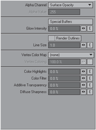
Figure 5-1
As compositing is really an entirely separate subject, I will not go into detail about it here. I recommend doing some research into compositing if you are not familiar with the process, as it is an extraordinarily important part of production.
NOTE: See Chapter 11 for more information about alpha channels.
There are four different options for setting the alpha for a surface.

Figure 5-2
Unaffected by Surface
Quite simply, this option causes the alpha channel to be totally unaffected by the object’s surface. Note that selecting this option results in the renderer treating the surface as a transparent surface, and the object does not appear in the alpha channel of the render at all.
Take a look at the following image. The glass surface of the lightbulb has been set up with this alpha option, resulting in the entire surface being excluded from the alpha channel.
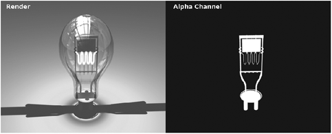
Figure 5-3
In this example, the ground plane object is also excluded from the alpha channel (simply because when it is included, the entire alpha channel appears white because of the position of this object).
Constant Value
This option allows you to enter your own value for the alpha. This value, however, is a constant, flat value, not allowing for any variations across the surface.
Even if the surface is totally transparent, if you set its alpha setting to Constant Value with a value of 255, it will be solid in the alpha channel, as in Figure 5-4.

Figure 5-4
Even though this object is glass, and is therefore transparent, the alpha setting of 255 (in other words, pure white) makes it solid in the alpha channel of the render.
Of course, you can set this value to anything from 0 to 255.
Surface Opacity
This is the default alpha setting. Surface Opacity basically takes all the information from the basic surface attribute settings of the transparency channel, and uses that to determine the values in the alpha channel. Any details that you have included in the Transparency Texture Editor that have variations in transparency will remain intact in your alpha channel as well, usually resulting in a more accurate channel for compositing.
In the following image, this setting is used on the bulb’s glass. Because the transparency of the bulb is set up using gradients to create a Fresnel effect (gradients are discussed in Chapter 9), the transparency of the bulb lessens at the edges of the glass. As you can see, this effect is taken into account in the alpha channel.
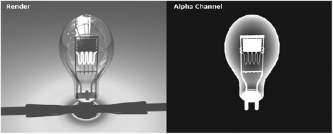
Figure 5-5
Any detail in the transparency channel, regardless of whether it is a gradient, a procedural, or an image, will affect the surface opacity and therefore the alpha channel.
Shadow Density
This alpha option is geared especially toward use in renders that will be composited with live action plates. Using Shadow Density will exclude the entire object from the alpha channel, except for areas where there is a shadow falling onto it.
So if, for example, you are working on an object that will be composited onto a surface on a live action plate, you could create a surface object that represents that surface in the filmed footage and use this alpha setting on it. That way, the object will not be included in the alpha channel, except for the areas where the object to be composited has cast a shadow on it. The following figure shows this option being used for the ground object. As you can see, the ground plane is not included in the alpha channel except for the area where the shadow from the bulb object is cast into it. The rest of the ground object is therefore ignored by the alpha channel.

Figure 5-6
Usually you would create a texture for the surface that is as closely matched as possible to the one in the filmed footage so that any colors that may be included in the shadow are carried over into the composited frames.
If we composite this render onto another image, we get the type of effect shown in Figure 5-7.
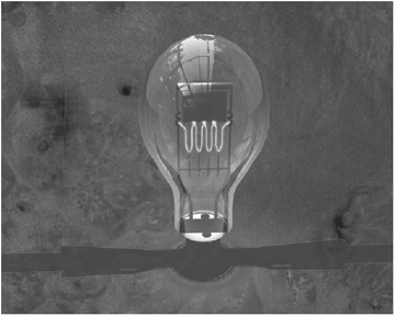
Figure 5-7
Although this is obviously a rough example, you can see how the shadow is then included when you composite using the alpha channel of the render.
Special Buffers
This option is rather mysterious for even many seasoned LightWave users. Just what on earth are special buffers? Honestly, this one took me a while to figure out.
Special Buffers are basically there to let you enhance your surfaces using some of the image filters found in LightWave. Since I discovered how to use them properly, I use them all the time!
To use Special Buffers, you need to have some processing filters set up in the Processing tab (in the Effects panel) in Layout (press Ctrl+F8 to get the Effects panel), under the Image Filter heading. There are only four filters that work with Special Buffers: Render Buffer Export (called just Buffer Export when added to the filter list), Corona, Full Precision Blur (called FP Blur in the list), and Soften Reflections.

Figure 5-8
Usually when these filters are applied in Layout, they affect everything in the render. However, these four particular filters can be isolated to affect only surfaces that are using them through Special Buffers, using the individual options in each, as illustrated in Figure 5-9.
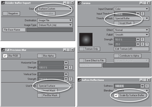
Figure 5-9
If you set these filters up as shown, they will not have a global effect when rendered. Instead, they will affect only those surfaces that are accessing them using Special Buffers.
Take a look at Figure 5-10. In this example, the Full Precision Blur filter has been added to the Effects panel, but has not been isolated to Special Buffers, as illustrated previously. As you can see, the blur is applied to the entire render.
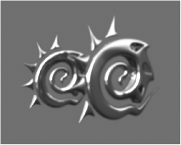
Figure 5-10: Using Full Precision Blur filter
Now, if we want to limit this blur to the logo at the back only, we can do so using Special Buffers.
As you can see in Figure 5-11, the blur effect of the filter is applied only to the logo at the back because that one is using Special Buffers. Pretty useful, eh?

Figure 5-11: Using Full Precision Blur filter with Special Buffers
So how exactly do we use Special Buffers then?
Well, it is fairly simple. Go the Advanced tab in the Surface Editor and click on the Special Buffers button. The Special Buffers Options panel opens.
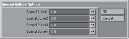
Figure 5-12
As you can see, there are four fields in this panel. Each of these fields corresponds directly to an image filter in the Effects panel. The first field in the Special Buffers Options panel works in conjunction with the first filter in the Image Filter list, the second field with the second image filter, and so on.
Obviously, since there are only four image filters that work with Special Buffers, there are only four fields. That is the simple part.
Actually using them properly requires a little bit of brain work. To best demonstrate how to use these buffers, let’s examine each of the four filters individually.
NOTE: Please note that these image filters are discussed in greater detail in Chapter 19. This chapter merely explores their interactions with the Special Buffers option.
Corona
Corona can use Special Buffers to control its Input Channel and Threshold Mask settings.
The Input Channel parameter in this particular filter determines what aspect of an object’s surface triggers the Corona effect, which is basically a very strong bloom effect, such as you get from very strong light reflections of certain types of surfaces.
If you select to use Special Buffer as the Input Channel, then this obviously causes the effect to only work together with any surfaces using Special Buffers.
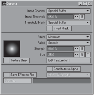
Figure 5-13
So, in this example, to get the Special Buffers to work with Corona, we will enter a value of 1 in the first field in the Special Buffers Options panel for this surface.
You may be wondering why a value of 1. Well, this is the part that gets a bit tricky, because this particular aspect of using Special Buffers is what differs from filter to filter.
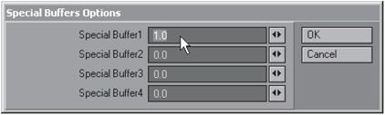
Figure 5-14
When using Corona, using a value of 0 will obviously result in no effect from the filter, whereas a value of 1 basically activates the filter. This particular filter does not work with any values other than 1 and 0. Choose 0 to essentially switch the buffer off, and choose 1 to switch it on.
Figure 5-15 is a rather extreme example of using Corona on the surface, using Special Buffer as the Input Channel in the Corona filter.
As I mentioned a moment ago, Special Buffers can also be used to control the Threshold Mask setting for this filter. This particular setting is used to limit the effect of the filter by masking it out based on input determined by what is specified as the mask. In this case, using this setting basically works opposite of the Input Channel setting. Selecting Special Buffer as the Threshold Mask will exclude any surfaces using them from the effect of the Corona filter.

Figure 5-15: Using Corona filter with Special Buffers
NOTE: Using the Special Buffer option as both the Input Channel and the Threshold Mask will result in no Corona effect, as they effectively cancel each other out.
Full Precision Blur
As we saw earlier, the Full Precision Blur effect can be controlled by Special Buffers simply to determine which surfaces it blurs. This is a pretty straightforward filter to use.
To use it, open up its panel by double-clicking on it in the Image Filter list in the Effects panel. Select Special Surface as the Use Mask option.
Using this filter with Special Buffers in the Surface Editor is a little different from the way that we used it with the Corona filter.
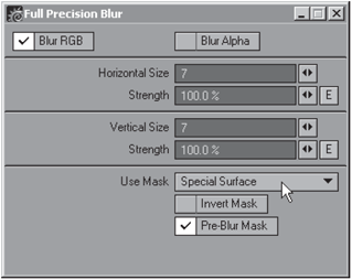
Figure 5-16
Take a look at the settings I have used in the blur. As you can see, I have used a value of 7 for both the horizontal and vertical blur.
To make sure that the surface blurs according to these values, we need to choose the correct Special Buffers value for it in the Surface Editor. In this case, I need to enter a value of 70.

Figure 5-17
You do not need to be a brain surgeon to understand how this works. In this case, I multiplied the value from the filter by 10 and entered the resulting value.
The funny thing is that even amounts like 20 look almost identical to this value, so entering a value of 70 was only really for absolute precision for the sake of an example. It is only when we start going down to values closer to 0 that we begin to see a noticeable difference.

Figure 5-18: Using Full Precision Blur filter with Special Buffers
Figure 5-19 shows a render using a Special Buffers value of 1.5.
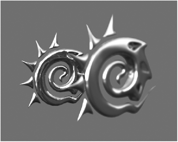
Figure 5-19
You may be thinking at this point that perhaps merely using the same values in the filter and the Special Buffers (in other words, for this example, using a value of 7 for both) would create the effect with precision. Well, the difference between using a value of 7 and a value of 70 is almost imperceptible, but it is there.
Render Buffer Export
This filter allows you to save images from LightWave’s internal buffers, which you select from the Source list. To use this filter with Special Buffers, use the Surface Custom option.

Figure 5-20
So what is this useful for? When used with the Destination option set to Rendered Alpha, you can use this filter, in conjunction with Special Buffers, to control the alpha values of different surfaces. Of course, the actual filter has other uses, but this is the only way that it can use Special Buffers. Not terribly exciting, but occasionally useful.
Although you can, of course, use your alpha setting in the Surface Editor to do this as well, using this filter to do this can be handy because it allows you to set up a save path to save the alpha channel separately. You control the actual gray value for this alpha with the Special Buffers amount in each surface.
Setting the actual value in Special Buffers for this filter, however, is not as simple as with the previous two filters that we have looked at.
As we all know, when dealing with gray values, 0 is black and 255 is white. However, despite this, the Special Buffers value in this case only ranges from 0 to 1. When entering values in this filter, 0 is black and 1 is pure white.
So, in order to enter the required amounts correctly, we need to do a little calculating. Luckily the calculation for this is not too complex. All we need to do is decide on a gray value from 0 to 255, as we usually would, and then figure out what percentage of 255 that value is and enter it into the Special Buffers field.
So if, for example, we wanted a gray value of 72, we would simply calculate it as follows: 72 / 255 = 0.28235.
We would therefore enter a value of approximately 0.28 in the Special Buffers field. This would result in the filter producing a render with the surface’s alpha channel being roughly equal to a gray value of 72.

Figure 5-21
Soften Reflections
The fourth and last image filter that works with Special Buffers is the Soften Reflections filter. Obviously this filter is for making reflections in surfaces appear softer, which is often a more realistic look, as we all know that really extreme, harsh reflections usually end up looking really fake.
To use Special Buffers with the Soften Reflections filter, simply select the Scale By Surface Buffer option in the filter’s panel.
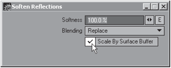
Figure 5-22
Using this filter in conjunction with Special Buffers is really straightforward. When using the Scale By Surface Buffer option, the amount you enter into the Surface Buffers field acts as a percentage of the value in the filter’s options. A value of 1 in Special Buffers will be 100% of the filter’s percentage; a value of 0 has no effect. Working out all the values in between is no major challenge, as they simply divide the filter percentage by 100.
Obviously, when using the Scale By Surface Buffer option, the filter affects only those surfaces that have a value entered into the corresponding Surface Buffer field. In Figure 5-23, the logo at the back is using its Surface Buffer to soften its reflections.
And that’s it for Special Buffers!

Figure 5-23
Glow
As the name suggests, this option is used to create a glowing effect on the surface to which it is applied.
To use it, simply enter a desired value for the glow.

Figure 5-24
This amount can be animated using envelopes, which is great for creating flickering glows. See Chapter 18 for more information on animating surface parameters.
In order for the glow effect to render, you have to activate it in your Processing options, found on the Effects panel in Layout (Ctrl+F8), by checking the little box labeled Enable Glow.
The Intensity setting determines how strong the effect will appear in the render, while the Glow Radius determines the size of the glow around the surface, in pixels.
You may wonder why there are settings for Glow Intensity on both the Surface Editor and the Effects panel. The answer is because the setting on the Surface Editor determines the percentage of the value on the Effects panel that the glow for that surface will have. In other words, if you have a Glow Intensity value of 50% on the Effects panel, and 100% in the Surface Editor, then that surface will glow at an intensity of 50%. If you set the value on the Surface Editor to 50% as well, the surface will glow with an intensity of 25% when rendered.
Using this option is great for making laser beams, evil glowing eyes, glowing skulls, and many other cool things.
Due to the nature of this option, it obviously works best with surfaces that have some degree of luminosity applied to them. See the “Luminosity” section of Chapter 4 for more information about using glow in conjunction with luminous surfaces.
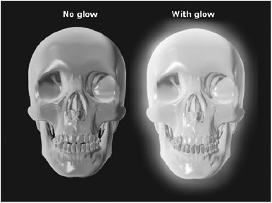
Figure 5-25
Render Outlines
The next option we find on the Advanced tab is Render Outlines. When this option is selected, the surface will render showing the outlines of the polygons instead of a smoothed version. This is basically similar to rendering a wireframe of the surface.
To use it, simply activate the option by checking the little box, and select an appropriate pixel width for the lines to be rendered.

Figure 5-26
Applying Vertex Color Maps
The Vertex Color Map option allows you to select and apply a vertex map that you may have made to the surface. Select the vertex color map that you wish to use from the drop-down list, and use the Vertex Coloring setting to determine the strength of the map. This amount can be animated.

Figure 5-27
See Chapter 7 for more information about creating and using vertex color maps.
Color Highlights
You use this option to color highlights on a surface according to the color of the surface itself. By doing so, you can lessen the harshness of specular highlights on a surface by allowing the surface’s color to essentially show through the highlights.
You can also use this option to tint reflections on a surface, which can be extremely useful for creating realistic reflections.
Using color highlights on glass is also great for lessening specular glare that can often ruin transparent surfaces.
This effect can be animated.
Color Filter
This useful option is for tinting transparent surfaces, thereby making everything you see through the surface appear tinted by the color of the surface to which it is applied.
For example, if you make a glass orange, you can use this setting to make everything appear orange when you look through that glass. Obviously the Color Filter option only works on objects that are transparent to some degree. This effect can be animated.
Additive Transparency
This setting can also only be used on transparent surfaces. It basically adds the color of the surface to which it is applied to the colors of objects that are seen through it, which creates the effect of the surface appearing much brighter by increasing its intensity. It is useful for creating surfaces that need to appear really blown out or overexposed, such as flames or other gaseous surfaces. This effect can be animated.
Diffuse Sharpness
Use this option for making the falloff of light on your surface harsher. It basically increases the contrast between the illuminated part of your surface and the non-illuminated part. Some surfaces, such as certain fabrics, can have this effect to a small degree, although you usually use it on objects that are rather large, like a planet that is totally devoid of light on the side that faces away from the sun (provided, of course, that said planet is illuminated by only one sun). This effect can also be animated.
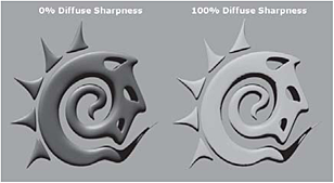
Figure 5-28
The Environment Tab
Setting Up Environments
The next tab that we encounter in the Surface Editor is the Environment tab. Using the options on this tab, we set up the reflection and refraction settings for your surfaces, as well as set up environments for those settings, should you require them.
Environments are basically there to give your reflective objects something to reflect if the actual environment in your scene is unsuitable or insufficient for any reason. You also use the Environment settings to specify how the reflective surfaces get their reflection when rendered.

Figure 5-29
Reflection and Refraction Options
Choosing Reflection Settings
We have a number of different options for setting up the reflections of the surface. The first thing that we need to choose here are the Reflection Options, which you select from a drop-down list. This determines what your surface actually reflects. You have four options.

Figure 5-30
The first option, Backdrop Only, causes the surface to only reflect whatever is in the background in your scene (you set up the background in the Effects panel in Layout). Using this option will have the surface ignore any geometry around it in its reflections.
Figure 5-31 shows the result of this, using an HDR image as the background in the scene. As you can see, neither the red cubes nor the ground plane appear in the surface reflections.

Figure 5-31: Backdrop Only reflection
The second option, Ray Tracing + Backdrop (which is the default), sets the surface to reflect everything that is around it (other models), as well as the background that you have set up in Layout. This usually gives the best results, as the entire scene is accurately reflected in the surface. See Figure 5-32.
This option takes slightly longer to render since everything in the scene is taken into account.
The Spherical Map option uses an image, which you select from the Reflection Map drop-down list, as an environment that is invisibly “wrapped” spherically around the surface and then reflected in it. Using this option causes the surface to ignore any surrounding geometry (like the Backdrop Only option), as well as the background in the scene. The only thing that we see reflected in the surface is the image that we select as the reflection map. Figure 5-33 uses this setting, with the same HDR image applied as the reflection map.

Figure 5-32: Ray Tracing + Backdrop reflection
When using a reflection map, we can control the rotation of this image by changing the Image Seam Angle setting.
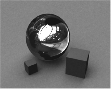
Figure 5-33: Spherical Map reflection
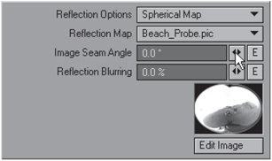
Figure 5-34
You use this setting because when images are wrapped spherically, as is the case here, there is invariably a seam at some point where the two ends of the image meet. Of course, you can create seamless images (we explore this in Chapter 11), but if your image does have a visible seam, you can adjust this amount to rotate the seam out of sight in the render. This value can be animated.
The fourth choice for Reflection Options is Ray Tracing + Spherical Map, which allows both the reflection map that you have chosen, as well as any surrounding geometry, to show up in the surface’s reflection.
As you can see in Figure 5-35, the image you are using as a spherical map acts in the same manner as a backdrop in the scene would work. When using this option, the surface totally ignores whatever the actual background is in the scene and instead uses the spherical image. However, you still retain control over the rotation of this image, just as with the normal Spherical Map option.
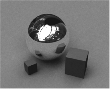
Figure 5-35: Ray Tracing + Spherical Map reflection
Choosing Refraction Settings
When using transparent surfaces, we have to deal with refraction. Luckily, setting up the refraction options is pretty simple to explain because your options are exactly the same as those we just looked at for reflections.
Please note that the following images all have a certain degree of reflectivity to them as well as a refraction index of 1.2.
Backdrop Only causes the surface to refract the backdrop image only. Any objects seen through the object are not refracted. This creates a rather unrealistic look, although it can be useful when there is no other geometry and you are looking straight through the object to the background.
Ray Tracing + Backdrop (which is the default) causes the surface to refract the backdrop as well as any surrounding geometry. Just as with your reflection settings, this option usually gives the best results, as the entire scene is accurately refracted through the surface; however, it also takes quite a while longer to render (refraction generally does take a long time to render anyway).

Figure 5-36: Backdrop Only refraction
Spherical Map uses an image that is refracted inside the surface. This option causes the surface to ignore any surrounding geometry (like the Backdrop Only option) as well as the background in the scene, which are not refracted at all through the surface. Due to the nature of refraction, this option is an extremely unrealistic one.
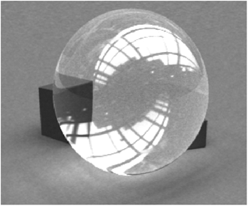
Figure 5-37: Ray Tracing + Backdrop refraction
You select the image from the Refraction Map list, and rotate it using Image Seam Angle just as you do with a reflection spherical map.
Ray Tracing + Spherical Map allows both the refraction map that you have chosen, as well as any surrounding geometry, to be refracted through the surface. Just as with your reflection option of the same name, the spherical map acts like a background image. Rays passing through the surface will bend and continue traveling until they hit any objects behind the refractive surface or the backdrop.

Figure 5-38: Spherical Map refraction
This option, like the Ray Tracing + Backdrop option, can cause your render times to increase rather dramatically.

Figure 5-39: Ray Tracing + Spherical Map refraction
Reflection and Refraction Blurring
Both your reflection and refraction settings panels have a Blurring option. Use this option with caution as it greatly increases render times. These values can be animated.
TIP: If you want to blur your reflections, but do not have the time to sit and wait for really long renders, consider using the Special Buffers option in conjunction with the Full Precision Blur filter, as discussed in the Advanced Tab section of this chapter.
Don’t forget that in order to have your reflections and refractions render correctly you need to activate Ray Trace Reflection and Ray Trace Refraction in your Render Globals panel in Layout.
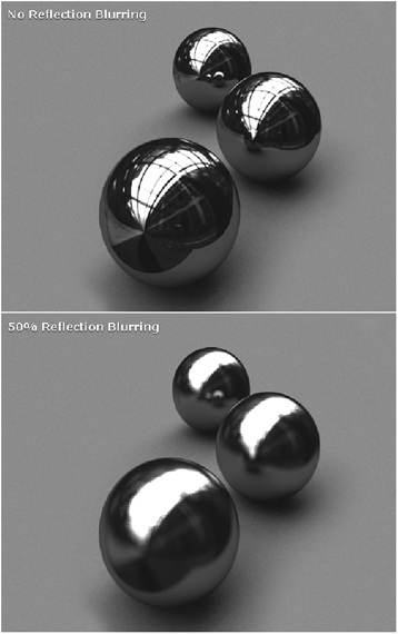
Figure 5-40
Shaders
Just what are shaders? This is a question that I get asked fairly often. I believe this is because this term is used in different ways from program to program. In some 3D packages, the term “shader” is used to describe any surface created and applied to a model, whereas in other programs, a shader is a special script written to give the surface certain qualities. Sometimes the term “shader” is confused with shading models, which are something else entirely. Shading models are basically mathematical models that determine how surfaces react to different lighting conditions. As LightWave users, we are generally not bothered by different shading models though, as LightWave only uses the Phong shading model.
In LightWave, a shader is a special plug-in that you add to your surface to give it certain properties, usually properties that define the manner in which light reacts to the surface, as opposed to actually adding details to the surface.
Just to clarify a bit further, the entire art of creating and setting up surfaces in CG involves two distinct steps: texturing and shading. Texturing encompasses all the processes of creating image maps, setting up procedural textures, and basically doing anything that creates details on the surface at hand.
Shading the surface is setting up the way that the surface reacts to light by defining the manner in which it reflects, absorbs, and scatters light. Sure, creating reflection maps and such can define where the surface is reflective, but the actual nature of that reflection (such as the tint of the reflection itself or the direction of that reflection, etc.) is controlled by the shading of the surface, which is set up separately. By using shaders in LightWave, we can apply global shading attributes to the surface as a whole without having to make changes in each of the surface’s individual channels.
NOTE: For more information on the difference between shading and texturing, refer to the end of this chapter.
While LightWave ships with a number of shaders included, there are also a large number of commercial shaders that one can purchase, as well as free shaders that you can download from various developers’ sites on the web.
Built-in LightWave Shaders
To add a shader to your surface, go to the Shaders tab in the Surface Editor and click on the Add Shader button. This presents you with a drop-down list showing all the shaders that you currently have installed in LightWave.
NOTE: This image shows only standard shaders that come with LightWave. If you have other shaders, and wish to use them, simply add them to LightWave, and they will appear in this list along with the others. See your LightWave manual for information on adding plug-ins.
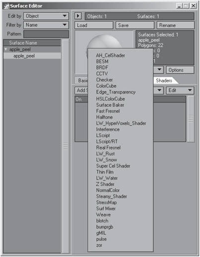
Figure 5-41
Selecting a shader from this drop-down list will add it to the shaders list in the Surface Editor. Within this shaders list, you can reorder, remove, copy, and paste shaders as you wish.
Double-clicking on a shader’s name in the list opens up its command panels, if it has one (some shaders do not have panels).
BRDF (Bidirectional Reflectance Distribution Function)
Yes, this shader has one of the most impressive names in the whole 3D field! Amaze your friends by dropping this term at important events, and then pretending that it is something really profound. Further amaze them with this really complex explanation:
The bidirectional reflectance distribution function gives the reflectance of a target as a function of illumination geometry and viewing geometry. The BRDF depends on wavelength and is determined by the structural and optical properties of the surface, such as shadow-casting, multiple scattering, mutual shadowing, transmission, reflection, absorption and emission by surface elements, facet orientation distribution, and facet density.
Just make sure that you look like you know what you are talking about when you say all that.
In terms of actual execution, the BRDF shader is actually quite simple. And the cool thing about this shader is that it can be used for a couple of different things.
Take a look at the shader’s interface in Figure 5-42.
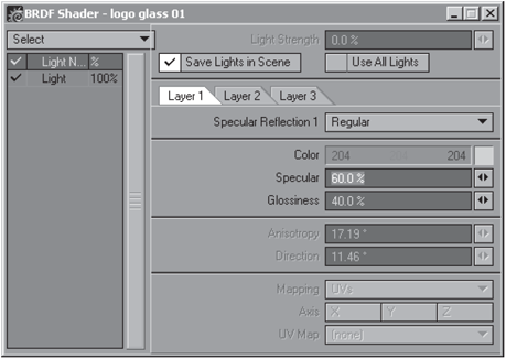
Figure 5-42
It looks a little complex, doesn’t it?
First, and most simply, you can use this shader to exclude certain lights within the scene from the surface. Notice the list on the left-hand side of the panel where all the lights in the scene are listed. You can check or uncheck each light in this list, depending on whether or not you want it to affect the surface. Just click on the little check mark next to the light’s name to disable it.
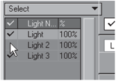
Figure 5-43
Selecting each light in the list also allows you to set values for the light’s strength on the surface. You can enter this value in the field labeled Light Strength.
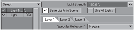
Figure 5-44
That is the first useful thing about this shader, although it is not the actual main intention of it. It is just one of those little things that you can use it for.
The main purpose of this shader lies in its ability to assign up to three different layers of specularity, each with different settings, onto the surface.
Why would we need to do this? Simple. Some surfaces have multiple layers of specularity, or at least appear to. Take a look at any lacquered surface, such as wood that has been varnished. How would you texture that? Sure, we could take a quick route and just make it nice and shiny, and a bit glossy as well. However, a more realistic approach would be to consider the properties of the wood and the properties of the varnish separately. Because surely, when you think about it in those terms, you realize that wood has a different specularity than varnish. In this case, you can use this shader to specify that the surface has a layer of low specularity (the wood), which is covered by a second layer that has a higher specularity (the varnish). Take a look at Figure 5-45.
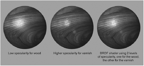
Figure 5-45
In this image, the first sphere shows the wood texture using just a normal low specular setting, as would be appropriate for wood. The second sphere shows a higher specularity and gloss setting, more suitable for varnish. The third sphere uses the BRDF shader to create two separate layers of specularity, each with specular and gloss settings appropriate for its substance.
Figure 5-46 shows the first layer of specularity. This is a broad highlight for the wood. I have used a color for the highlight here as well, as wood tends to have a lot of its own color in its specularity.
Figure 5-47 shows the settings for the second layer in the BRDF shader, the layer that gives the specular look to the varnish on the wood.

Figure 5-46

Figure 5-47
As you can see, this has higher specular and gloss settings and is set to pure white so that it is nice and shiny. In the render that we saw previously, this creates a nice glossy highlight on top of the broader, duller highlight, just as varnish on wood would do.
This example uses only two layers of specularity, but the shader does allow up to three layers that you can stack on your surface.
All these examples have used the Regular option of the Specular Reflection setting. Now let’s delve into the other types.
The third use for this shader is for applying anisotropic shading to your surface’s specularity. Anisotropic shading is useful for when you are creating surfaces such as brushed metal, where the surface is covered by tiny grooves that break up the light, consequently causing a distortion in the reflections and highlights on the surface.
The BRDF shader offers two types of anisotropy: Anisotropic (controlled by two angles of disturbance) and Anisotropic II (which uses mapping coordinates to control the disturbance).

Figure 5-48
Anisotropy is defined with two values, Anisotropy and Direction, both of which are measured in degrees. The Anisotropy value sets the angle along which the “grooves” in the surface lie, while the Direction value determines the angle at which light will gather in these grooves.
Figure 5-49 shows a sphere with an Anisotropy setting of 0° and a Direction value of 90°. As you can see, this causes the light to gather perpendicular to the direction of the Anisotropy.
This setting would be ideal for a brushed metal surface such as typically found on lava lamp bases or stainless steel kitchenware.
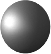
Figure 5-49
Figure 5-50 shows the same sphere with the settings switched around, so the Anisotropy value is now 90° and the Direction value is 0°.
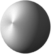
Figure 5-50
As you can see, the results are rather different. This type of setting almost emulates a radial anisotropy such as you find on the knobs of a hi-fi system.
The Anisotropic II option allows you to use either Cylindrical, Cubic, or UV parameters to define the anisotropy.
The Cylindrical and Cubic mapping types are shown in Figure 5-51. The Cylindrical option allows you to select an axis along which the anisotropic effect will project.
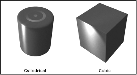
Figure 5-51
The UV option allows you to use a selected UV map as the method of defining the anisotropic effect. The way that this option works is that it looks at the way in which your UV map is constructed and determines the direction for the effect. You alter the effect and create patterns by flipping the points within your UV map in Modeler, using the Flip UV Point Map command, or by manually rotating parts of the map around.
Figure 5-52 demonstrates this. The cube has been UV mapped and every other block in the UV map has been rotated. As you can see, this forms a checkerboard type pattern where the light hits the surface, even though there is no such texture applied to the model. This is because the anisotropic effect is now defined by the coordinates of the UV map, and since some of those points have been flipped, the effect becomes flipped.
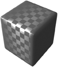
Figure 5-52
You may wonder how this could be useful. Well, you could use this to create iridescence in surfaces, or simply to create other unusual patterns of light.
Edge Transparency
This particular shader is only for use with surfaces that are already transparent to some degree, as its purpose is to define the clarity of transparent edges. This is especially useful for clear transparent surfaces that often tend to lose clarity when placed in front of other objects or a backdrop.

Figure 5-53
Take a look at Figure 5-54. The logo on the left is a simple transparent surface, while the logo on the right uses the Edge Transparency shader (with default settings). As you can see, the shader creates edges that appear solid to a certain degree, using the surface’s color.

Figure 5-54
The shader gives you three different types of blending for the edges: Opaque (the default), Normal, and Transparent.
The Opaque option (shown in Figure 5-54) creates an adjustable black semisolid-looking edge, while Normal subtly creates the appearance of a totally solid, hard edge. Transparent makes the edges blend completely away with no definition whatsoever. Both the Opaque and Transparent options have an Edge Threshold setting that you can adjust to vary the amount of blending between the surface’s color and the transparency at the edges.
Figure 5-55 shows each of the types using default settings.

Figure 5-55
Use Edge Threshold to soften or harden the edges by increasing or decreasing the value, respectively. The following image shows a low value and a high value of Edge Threshold using the Transparent type.
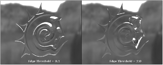
Figure 5-56
Surface Baker
The Surface Baker shader is an extremely useful little thing. Have you ever created a really cool procedural texture in LightWave but wished you could somehow manually paint some more details into it? Or have you ever wanted to somehow add the highlights and shadows from your scene lighting into your textures for a game model? This is what the Surface Baker shader is for. You essentially bake your textures and/or lighting information (this includes all highlights and shadows, and even caustics and radiosity) to an image (using a UV map) or directly onto your object’s vertices.
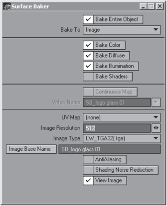
Figure 5-57
To use the Surface Baker, simply assign it to your surface, set it up as desired, and render your image. The image baking will occur before the camera rendering takes place. Once the baking is done, the image is saved to a selected destination, and the rendering of the actual scene (through the camera) follows.

Figure 5-58
Let’s have a look at all the options this shader gives us.
At the top of the shader’s panel we have the Bake Entire Object option. Checking this option will bake all the surfaces of that entire object instead of only the surface to which it is applied.
This is particularly useful when baking the effect directly to a vertex map assigned to the entire model (using the Bake To Object option, discussed next), since it saves time.

Figure 5-59
Next, we have the Bake To option, which gives us two choices from a drop-down list: Image and Object.
The Bake To Object option bakes all the texture information to a vertex color map that you enter or select from the VMap Name field.
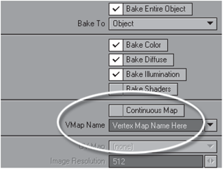
Figure 5-60
Checking the Continuous Map option above the VMap Name field turns on polygon smoothing so that the map is smoothly interpolated between vertices (basically it is the same as the Smoothing option found in the Surface Editor, discussed in Chapter 3). Deselecting the option will result in sharp changes at the vertices, which is the effect you would probably want if you were baking the textures of objects like walls or a sharply edged object that you wouldn’t want to have smoothing applied to.
Once you have created the baked vertex map you can apply it to the surface by going to the Advanced panel in the Surface Editor and selecting it from the Vertex Color Map drop-down list.
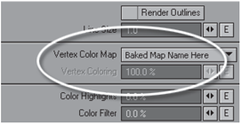
Figure 5-61
The Bake To Image option lets you choose a UV map (previously created in Modeler) to which the textures will be baked. When baking to an image, you have options to select which UV map you wish to bake to, what image resolution you want the baked texture to be, and what type of image (format) you’d like LightWave to save the image as.

Figure 5-62
NOTE: When saving the resulting baked image as a 32-bit texture, please take note that the wireframe of the UV map is included in the alpha channel of the image. Many people get a bit confused when they apply the baked image as a texture to their model, only to find upon rendering that the image looks really bizarre. If you find this happening, simply open the Image Editor and disable the alpha channel.
Select the UV map from the UV Map drop-down, which lists all UV maps that are currently created for that model. Enter an appropriate image resolution for the baked image. This determines the actual pixel dimensions (width and height) of the image. Remember that larger images are better quality, especially for close-up shots. Choose the format you wish to save the image as from the Image Type list, and enter a name for that image in the Image Base Name field. Clicking on the Image Base Name button allows you to browse for a destination to which LightWave saves the image upon rendering.
When baking textures, you have four basic options for what you actually want to bake into the baked image or vertex color map: Color, Diffuse, Illumination, and Shaders.

Figure 5-63
You can select any or all of these options when setting up the shader. Selecting Bake Color bakes all textures assigned to the Color Texture Editor in the Surface Editor.
Figure 5-64 shows a painted texture combined with some procedural textures that have now been baked into a single image.
The Bake Color option includes any images or procedural textures, as well as any gradients except view-based Incidence Angle (camera angle) gradients. This is because it is pointless to bake details that are dependent on viewing angles into a flat image. You can, however, bake Light Incidence gradients into an image.
The Bake Diffuse option bakes any diffuse shading (textures applied to the Diffuse channel) from the surface into the image.

Figure 5-64
Selecting this option alone creates a plain texture, but when using this together with the Bake Color option you’ll notice a considerable difference.
Figure 5-65 shows the color textures from the previous example now combined with Bake Diffuse. A procedural texture that was assigned to the surface’s Diffuse channel is now included in the image. Notice that the image is now somewhat darker from the inclusion of the diffuse shading.

Figure 5-65
Bake Illumination bakes all lighting and shadows from the scene into the textures. This option is great for situations like game environments, where you can simulate all the lighting effects in your textures without having to use real-time lighting in the game engine for this purpose. This option will include all kinds of shadows, radiosity, and caustics from the scene in the image. Only use this option if you want shadows and highlights in your textures. Ordinarily, we wouldn’t use this option for visual effects or animation, as it will create lighting discrepancies, especially if the character or object starts moving around.
Figure 5-66 shows the same textures from before with the lighting from the scene included by using the Bake Illumination option.
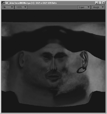
Figure 5-66
Lastly we have the Bake Shaders option. As its name suggests, this option simply includes any applicable information from shaders assigned to the surface into the baked image. Of course, once again, incidence-based shaders like the Fresnel shaders cannot be baked since their effect is dependent on viewing angles that make them useless in a flat image.
At the bottom of the Surface Baker panel we find two options for refining the quality of the baked image — AntiAliasing and Shading Noise Reduction — as well as the View Image option.

Figure 5-67
AntiAliasing smoothes the image (exactly like using antialiasing on your camera when rendering). While it does add to your rendering time, it produces a much better quality image. Shading Noise Reduction applies a low-level blur to the final image to reduce any grain that might appear within the image. This is particularly applicable when baking illumination, especially radiosity. It is exactly the same as the setting of the same name found in your Global Illumination panel in Layout.
Check the View Image option to have the image open in the Image Viewer once it has been rendered.
Fast Fresnel and Real Fresnel
The Fresnel effect is discussed a number of times in this book, but to save you the hassle of paging through all the chapters trying to find an explanation, I’ll repeat it here once again.
Named after the French physicist Augustin Jean Fresnel, the Fresnel effect is the phenomenon that we observe in the real world whereby the amount of reflection that we see on a surface differs according to the angle at which it is viewed.
Look at the sea as an example. When we are standing in the ocean looking straight down into it, we can see all the way to the bottom. However, as we move away from the sea, and view it from a distance, it appears to be very reflective, as the angle that you are looking at it has decreased. When the sea is on the horizon, far away in the distance, it appears to be almost mirror-like, so that if you never saw it up close, you would never think that the water was actually almost completely transparent.
A common example of this effect can be observed in any glass object. Take a look at a glass, and you will notice that the edges of the object appear far more transparent as they slope away from your direct angle of vision.
We have two shaders in LightWave to create this effect. Let’s look at Fast Fresnel first. Figure 5-68 shows the Fast Fresnel shader’s control panel.
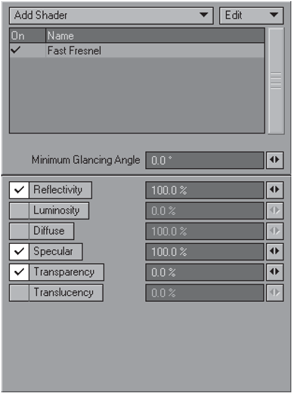
Figure 5-68
While the Fresnel effect in reality is concerned with reflections and refractions of light, we can use the Fast Fresnel shader to apply incidence-based effects to any of the surface properties listed, namely Reflectivity, Luminosity, Diffuse, Specular, Transparency, and Translucency.
Above the properties we have a field labeled Minimum Glancing Angle. This value determines the beginning value from which the effect will be measured. Generally, this value would be 0° since that is the angle at which we view a surface straight on, and having the effect measured from 0° also gives us the widest spread of the effect (which is measured up to a maximum of 90°).

Figure 5-69
The maximum value for this effect is 89° (since this is the area of the surface that slopes out of our vision), so entering a value of 90° in this field would nullify the effect.
Next to each of the surface parameters are fields where you can enter values from 0% to 100%. This basically controls the intensity of the effect for that particular surface property when it reaches the higher glancing angles (90°).
For example, if we leave the reflectivity value at 100% (default), then the reflectivity of the surface will increase from whatever value is assigned to the Reflection channel (in the Surface Editor) to a maximum of 100% at the edges of the surface where it slopes away from our vision.

Figure 5-70
So basically this value determines the strength of the effect in that channel on the edges of the surface. While this particular shader has no option for affecting the Glossiness, Color, or Refraction channels, we can fake the effect using gradients. This is discussed in depth in Chapter 9.
NOTE: It is worth mentioning that when using the Fast Fresnel shader, LightWave’s renderer treats your surface as a transparent surface, even if there is no degree of transparency applied to it. This means that the surface takes slightly longer to render than usual.
Moving on to the Real Fresnel shader, we find a much simpler-looking shader interface, as shown in Figure 5-71.
This shader has fewer settings because it is based on realistic physics, as opposed to the Fast Fresnel shader that is basically a quick-and-dirty Fresnel solution.

Figure 5-71
This shader automatically makes your surface transparent when you add it to the shader list and calculates the transparency falloff using the Fresnel algorithm.
The Reflective Polarization and Specular Polarization settings determine the values for those two particular surface attributes when the camera is perpendicular to the surface (90°). This means that the higher these values, the stronger the effect (in much the same way as the glancing angle values worked in the Fast Fresnel shader).
The following figure shows the effect of this shader. The sphere on the left has 100% specular polarization and 100% reflective polarization, while the sphere on the right has 0% specular polarization and 50% reflective polarization.
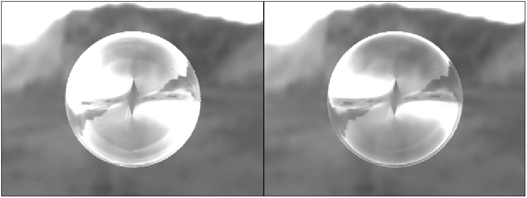
Figure 5-72
Halftone
The Halftone shader simulates the look of half-tone screens used in printing, which create the illusion of continuous shades of color with patterns of dots. The shader adds selectable patterns in black to the surface color specified in the Surface Editor.

Figure 5-73
You have a number of different options for determining the look of the effect on the surface.
The Spacing and Variation values determine the spacing between the patterns and the variations within them along the x- and y-axes. Higher values of variation create a more random patterned effect.
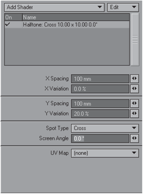
Figure 5-74
Figure 5-75 demonstrates the effect of increasing these values. The cube on the left has 200% for both X and Y Spacing and 0% for X and Y Variation. The cube on the right has 400% for both X and Y Spacing and 25% for X and Y Variation.
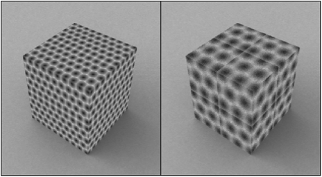
Figure 5-75
The Spot Type drop-down list gives you eight different patterns to choose from: Dot, Soft Dot, Block, Cross, Scale, Chex, Line, and CrossHatch.

Figure 5-76
The Screen Angle field allows you to change the angle (horizontal angle) of the dot pattern. In the following image, the cube on the left has a Screen Angle value of 0° while the cube on the right has a value of 45°.
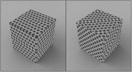
Figure 5-77
The final option is for using a selectable UV map to determine the direction for the cross-hatch or line pattern types. When you are not using a UV map for this, the patterns are applied to the surface in a cubic projection.
Interference
This shader simulates the weird rainbow effect that we see on oil slicks, where light is reflected between two substances (water and oil) that are of different thicknesses. The shader creates a spectrum of colors in a banding fashion to the surface, using incidence angles to vary the visibility of the different colors.
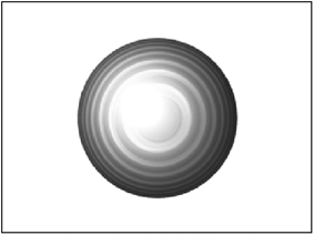
Figure 5-78
Controlling the shader is relatively simple, since it has only a few parameters that determine the nature of its effect.
The Spectrum Scale and Angle Range settings control the colors and position of the effect. The percentage entered into the Spectrum Scale field determines how much of the visible color spectrum will appear on the surface. The entire visible color spectrum consists of red, orange, yellow, green, blue, indigo, and violet. Selecting 100% will show all seven colors. A lower value will display fewer colors.

Figure 5-79
The Angle Range values (Min and Max) specify the position of the spectral effect by determining the minimum and maximum incidence angles between which the entire spectrum specified by the Spectrum Scale percentage will travel.

Figure 5-80
For example, if you leave the shader on its default settings (42° and 50°) with a 100% Spectrum Scale value, then all seven of the spectral colors (red, orange, yellow, green, blue, indigo, and violet) will appear between 42° and 50° on the surface (and will repeat themselves to the edge of your view of the surface as well).
However, if you were to change the minimum and maximum values to 0° and 90° (respectively), then the spectrum will appear only once, and will begin at 0° and end at 90°.
This is shown in Figure 5-81, where the sphere on the left has the default settings and the sphere on the right has the settings just described.
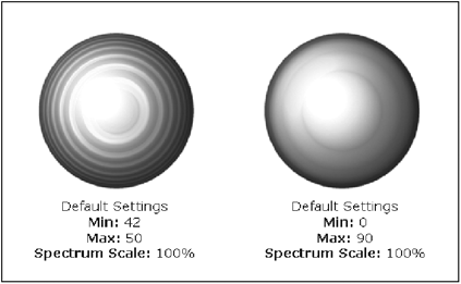
Figure 5-81
Selecting the Single Band option displays the spectral colors within a single band between the angles specified in the Min and Max fields only, instead of repeating themselves over the entire surface.

Figure 5-82
The Color Mode option gives you three ways of blending the actual effect with the colors of the underlying surface (created in the Surface Editor). You can choose from Add, Multiply, and Blend.
The Add and Multiply options are much the same as the Additive and Multiply blending modes we find in the Texture Editor (discussed in depth in Chapter 13).

Figure 5-83
Using the Add option, the RGB values of the colors are literally added to the underlying colors. The Multiply option multiplies the RGB values by a value from 1 to 0, depending on what value each pixel has. For example, any pixels with an RGB value of 255 (white) are multiplied by 1, while pixels with an RGB value of 0 (black) are multiplied by 0. All values in between are multiplied by a corresponding value determined by an even sliding scale between 0 and 1.
The third option, Blend, uses the percentage value in the field below to determine an even blend between the colors of the shader and the colors of the underlying surface. A blend of 100% makes the colors of the shader totally opaque, while lesser values blend them more with the surface itself.
Super Cel Shader
Cel shading is a method of rendering your surfaces to look like they are flat and 2D, just like a cartoon. Cel is the term given to the individual frames of hand-drawn animation. Television shows like Futurama use cel shading to great effect for integrating parts that are actually done in 3D into the 2D animation of the show itself.
This particular shader simply alters the renderer’s shading algorithm so that the surface no longer has smooth transitions between colors, turning them instead into flat bands of color.
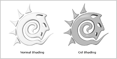
Figure 5-84
For best results, any objects being used with this shader should also be used with the Silhouette Edges, Unshared Edges, Sharp Creases, and Surface Borders options selected from the Edges tab of your Object Properties panel in Layout.
The overall effect of the shader is determined by defining the appearance of color zones that create the differences in shading on the surface. Basically, these define the zones where the shading will appear to change so that you can have variations on the surface that give the impression of form and shape.
A maximum of four zones can be defined on the surface from the shader’s panel, each with its own brightness settings. (See Figure 5-86.)
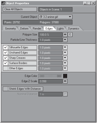
Figure 5-85
The Min and Max settings essentially define the different color zones on the surface, while the Brightness value for each zone is the amount by which the underlying pixel values of the surface are multiplied to create a flat, shaded color. Zone 1 represents the darkest zone (since it represents the areas that are in shadow), while Zone 4 is the lightest, so the brightness values should get progressively higher from Zone 1 through Zone 4.

Figure 5-86
The way in which the Min and Max settings actually define the color zones is that their values determine the brightness values between which that zone will appear. While the actual Brightness value determines the color shade (diffuseness) of that region (zone), the Min and Max values set the beginning point and end point of the overall brightness shading of the entire surface between which that zone will be active.

Figure 5-87
So if we think of the entire surface consisting of shades that fall between 0% and 100% brightness (influenced by the lighting in the scene), then the Min and Max values determine where color zones will start and end within that range.
Naturally this means that each progressive zone should begin (its Min value) shortly after the end of the previous zone (previous zone’s Max value). Keeping a difference of a few percent (5% to 10%) between the progressive Max and Min values of each zone softens the transition between each zone slightly.
Figure 5-88 shows the difference between keeping a 10% difference between zones (the logo on the left), as opposed to having no difference from the Max of one zone to the Min of the next.
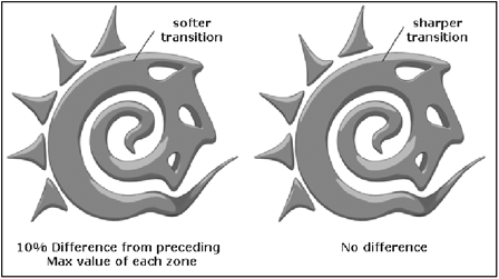
Figure 5-88
As you can see, the difference between the two is quite slight but still noticeable (hopefully!).
It’s interesting to note that essentially we could create exactly the same effect using a Light Incidence gradient in the color Texture Editor of your surface by specifying zones within the gradient ramp that change according to their relative position to the light.
Using a gradient would actually allow you to specify even more zones, as well as choose any colors you want, but the shader is generally more convenient.
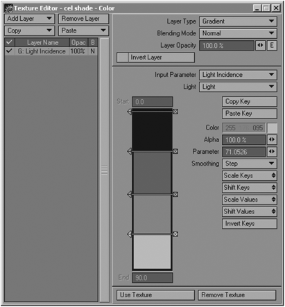
Figure 5-89
NOTE: See Chapter 9 for more information on gradients.
Once we have defined the color zones on the surface, the shader offers a few more options for the overall shading effect.
The Use Light Colors option allows you to use the scene lighting to tint the surface. Usually the color would come directly from the surface’s color as specified in the Surface Editor or from any texture applied to it.
Using the Specular Highlights option creates cartoon-like highlights on the surface, over and above the defined color zones.
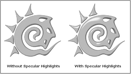
Figure 5-90
Use the Min and Max values to determine the appearance of the highlights by specifying which part of the specular highlight to show. A value of 0% represents the darkest part of the specularity, while 100% represents its brightest. However, using such a broad range tends to make the highlights difficult to see. Using a tighter range creates stronger, more noticeable highlights on the surface. The smaller the difference between the Min and Max settings, the harder the edge of the highlight becomes, so using the same values for both creates a very hard-edged highlight while having a large difference between the two creates very soft-edged ones, as shown in Figure 5-91.
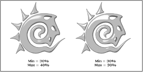
Figure 5-91
Using higher Min values creates smaller highlights, while lower values create broader ones.
Use the Brightness value to determine the overall brightness of the highlight itself, and the Saturation value to add the surface’s color to the highlight (similar to Color Highlights in the Surface Editor).
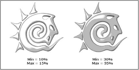
Figure 5-92
The final option, Bumped Edges, allows you to soften the appearance of the cel shaded object’s edges to avoid the very harsh look that they sometimes have. This option is an incidence-based effect that makes the edges appear slightly fuzzy and soft.
Since it is an incidence-based (viewing angle) effect, the Limit value defines the minimum angle that a surface normal has to be facing in order to be affected, where 100% represents areas facing directly at the camera and 0% represents the areas that are sloping away from it (the visible edges).
As the Limit value increases, the effect “creeps” inward from the edges of the surface, as shown in Figure 5-93.
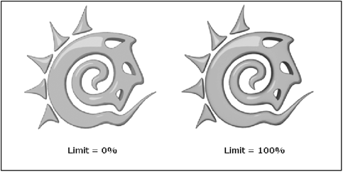
Figure 5-93
The Strength value determines how strong the effect is at the edges. Higher values have the effect encroaching a lot more on the edges. This value can go higher than 100%, but doing so tends to make the surface look less 2D. (See Figure 5-94.)

Figure 5-94
Thin Film
The Thin Film shader is very similar in effect to the Interference shader in that it also creates a spectrum of colors on the surface that change according to the camera’s angle in relation to the surface and can be used for effects like a film of oil on water.
The interface of the shader has some similar options to those found in the Interference shader, as well as some new ones for determining the actual colors and their position.

Figure 5-95
The Primary Wavelength value specifies the color in the spectrum that the shader uses as its base color. You can type a value into the field or simply click on a position on the actual color spectrum on the shader panel.
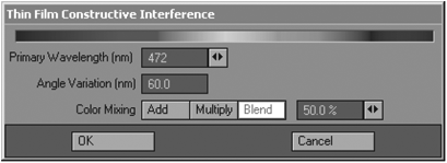
Figure 5-96
Use the Angle Variation value to determine the (incidence) angle at which the colors begin to shift. Higher values will begin the shift at the areas of the surface that are closer to perpendicular angles to the camera, while lower values have the shift occurring nearer the edges (the angles that slope away from the camera).
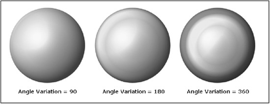
Figure 5-97
The Color Mixing options work in exactly the same way as the Color Mode options in the Interference shader.
Using the Add option, the RGB values of the colors are literally added to the underlying colors. The Multiply option multiplies the RGB values by a value from 1 to 0, depending on each pixel’s value. For example, any pixels with an RGB value of 255 (white) are multiplied by 1, while pixels with an RGB value of 0 (black) are multiplied by 0. All values in between are multiplied by a corresponding value determined by an even sliding scale from 0 to 1.
The third option, Blend, uses the percentage value to determine an even blend between the colors of the shader and the colors of the underlying surface. A value of 100% makes the colors of the shader totally opaque, while lesser values blend them more with the surface itself.
Z Shader
Probably one of the simplest shaders to use, the Z Shader allows you to change surface attributes based on their distance from the camera (much like the Distance to Camera gradients discussed in Chapter 9).
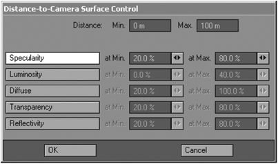
Figure 5-98
Use the Distance Min and Max settings at the top of the panel to specify the actual physical distance range (in units of measurement) from the camera that the shader will use as its input.
Once you have defined these two values, simply assign desired values to the minimum and maximum settings of the Specularity, Luminosity, Diffuse, Transparency, and Reflectivity attributes.
For example, if you have your Distance Min and Max settings at 0m to 100m, and you set your Specularity Min and Max settings to 5% and 100%, then at 0m from the camera, your surface will have 5% specularity, and at 100m from the camera, the surface will be 100% specular. All values between are interpolated.
Simple as that.
Surface Mixer
A relatively new shader for LightWave, the Surface Mixer allows you to blend two surfaces together. Since this effect can be enveloped, it is useful for animating changes in surfaces without actually morphing objects.
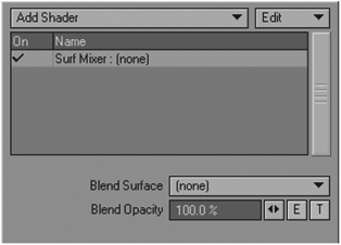
Figure 5-99
Simply select the surface that you want to mix the current surface with from the Blend Surface drop-down list (note that you can only blend with surfaces of other objects that are currently in your scene) and specify the Blend Opacity, which essentially determines how much the surface blends with the selected one. This value can be enveloped (click on the little “E” button to open the Graph Editor), as well as opacity mapped with a texture by clicking on the Texture Editor button (the little “T”).
gMIL Occlusion
The gMIL Occlusion shader was created by Eric Soulvie. Very little information about this shader is available aside from what is found in the LightWave manual.
Essentially, occlusion is a global illumination solution for determining how much ambient lighting is affecting any part of a surface. It figures out how “accessible” a surface is to ambient lighting in the scene and affects the surface accordingly.
Using this shader is similar to using the Backdrop Only radiosity mode in LightWave, although since you apply the effect using the shader, you can limit the effect to certain surfaces only, which can save time when rendering if you do not require global radiosity in your scene. Using gMIL is also faster than using radiosity because it is essentially a simulation effect and not a true radiosity calculation as such (in fact, occlusion is not actually radiosity at all, but rather an alternative, advanced lighting solution).

Figure 5-100
Looking at the settings in the shader’s panel, the first two options are Colour Add and Luminous Add. Essentially, these determine the overall strength of the shader effect by adding color and luminosity values from the scene (and backdrop) to the surface. Setting these values to 0.0 cancels the effect entirely.
Luminous Add obviously gives a certain degree of luminous quality to the surface, while Colour Add creates a stronger reflection of colors of the backdrop to the surface.
Take a look at Figure 5-101. The logo on the left has values of 0.1 for both Colour Add and Luminous Add, while the logo on the right has values of 0.5 for each.

Figure 5-101
Below these options we have some settings for controlling the falloff and samples of the shader. You have two options to choose from to determine the way in which the occlusion falloff is calculated: Linear and y=x^2. Falloff is the manner in which the light shades the surface when it hits it, as it darkens the surface while traveling farther from the source of light. Linear gives a totally linear (smooth) shading effect, while y=x^2 darkens the shadows slightly by squaring the effect. The difference between the two options can be almost totally imperceptible, though.
Next up we have options for controlling the effect of the sampling. The Sample Rate value determines the quality of the shading, although this does mean that higher values increase render times.

Figure 5-102
The Sample Style option lets you choose between Random and Ordered. Random (the default) gives you slightly rough, dithered shading, while Ordered creates a softer effect. Again, the differences between these two options can be almost imperceptible, depending on lighting conditions.
At the bottom of the panel are the actual occlusion options for diffuse, specularity, and reflection. You can activate (or deactivate) occlusion shading for each of these surface properties, as well as invert (the Inv. option) the effect for each. Inverting the effect is basically like inverting the falloff, so the entire surface becomes dark.
The following image shows the logo on the left with all three activated, while the logo on the right has the effect inverted on each.

Figure 5-103
Stress Map
Another great shader that will help you in the texturing process is the Stress Map. This shader will help you show strain or resistance on your polygon objects based on the amount of distortion applied to them via scaling, bone deformations, morph maps, and dynamics.
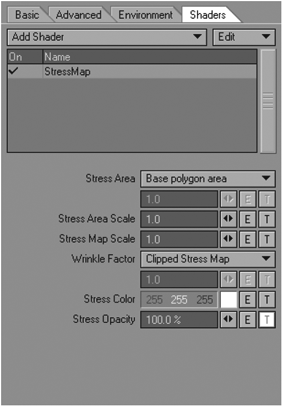
Figure 5-104: Stress Map options panel
You can use it to show wrinkles in the area being squeezed when bending the object with bones, or by having the wrinkles slowly vanish as the mesh is stretched, for example. You can also apply color to the stressed area and therefore mimic the discoloration of a plastic pipe when it is bent or a rubber band getting really stretched. (Think Wile E. Coyote trying to propel himself with a giant slingshot!)
The Stress Area setting determines the presumed local skin area if you are using wrinkles. If you set it to Custom you can use a texture, gradient, etc., to drive the size of the area. If you keep it at its default, Base polygon area, it will be equal to the undistorted mesh unless you scale it using the Stress Area Scale option. If you notice that your wrinkles are a little too subtle, you can increase its strength by increasing the Stress Map Scale value. This value will also scale the Stress Color if you are using that feature, so if you notice that the color has increased you may have to fine-tune the texture or gradient that drives the Stress Color to bring it back to what you previously had.
When creating wrinkles, the Wrinkle Factor is set by default to Stress Map, which controls how much bumps will show on the skin area. Sometimes it is more visible than it really should be, giving the impression that the skin is stretched beyond the breaking point. To correct this, set the Wrinkle Factor to Clipped Stressed Map, which will correctly display the bumps in the local stressed area only.
As I mentioned earlier, you can select a color or you can use textures for the stressed area using the Stress Color options. Stress Opacity will control where and how much of the color is visible in the stressed area. Figure 5-105 shows a plastic pipe being bent by the invisible man, with no stress, Stress Map Wrinkle Factor, and Clipped Stress Map Wrinkle Factor. This scene is on the companion CD for you to play with (TutorialsScenes 5.1-stress map.lws).

Figure 5-105
And that basically sums up LightWave’s native shaders.
Third-Party Shaders
There are a number of commercial and free third-party shaders available for LightWave as well. Many of the free ones are developed by prominent members of the LightWave community, and can be found by looking through LightWave community sites like Flay.com or NewTek’s forums. Some of the most popular commercial shaders are developed by Worley Labs and Evasion|3D, and can be investigated and ordered from their web sites.
The Difference between Shading and Texturing
We now know what shaders in LightWave are, and we have had a good look at each of the surface attributes that we deal with when creating surfaces, but before we delve into the world of creating textures, I thought it important to add a note about the differences between shading and texturing.
Put simply, the art of creating surfaces involves three distinct stages: mapping, shading, and texturing.
Mapping
Mapping, as we discuss later on, is the process whereby we set up coordinates on the surface so that we can correctly apply texture images (and procedural textures sometimes as well) to the model.
This is obviously a good place to start the surfacing process since it essentially creates a template upon which we will create our textures. When I am working on a project, I generally do all my UV mapping and sorting out of projections before I even consider taking the model into Layout for any test rendering.
Of course this is really a choice of habit, but I find it very efficient and it helps to keep me focused, as in my experience I’ve often found that people who are constantly rendering during the modeling and mapping process tend to waste a lot of time. What is the point in rendering an unfinished model?
Once I am satisfied with the creation and editing of any UV maps for the model, I am ready to take the model into Layout for shading.
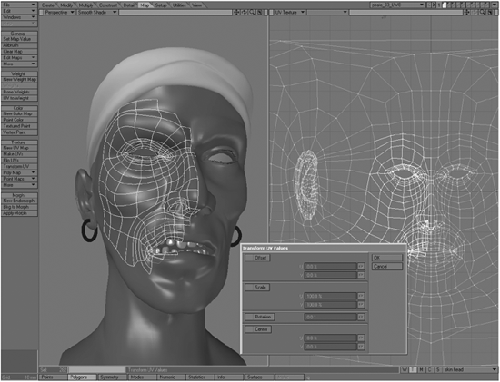
Figure 5-106
Shading
Shading is the crucial stage of the process whereby we begin to set up our lighting and start assigning basic values to each of the model’s surface parameters (its color, diffuse, specular, reflection, etc., parameters) so that it reacts to light correctly.

Figure 5-107
At this stage, there really should be no textures added to the model yet. Naturally, it is important to do one’s shading and lighting at the same time, since surfaces can be very sensitive to their lighting, and often require shading changes if the lighting changes in any way. Essentially, shading should define the way in which the surface looks and interacts with its environment and lighting, with the exception that at this stage, the surface has no details on it.
Shading is generally the trickiest part of the process. Determining the correct values for each of your surface’s attributes can be a painful process of tiny tweaks and waiting for renders. No two texturing situations are ever the same, so there is no foolproof “recipe” that will always work for any particular type of surface. Of course, as you become more experienced, you do begin to develop a good sense of how to start off the shading process speedily, but even so you’ll still find that this stage can be a challenge.
Of course at this stage you might find it necessary to employ some of LightWave’s shaders or even some of the gradients found in the Texture Editor (see Chapter 9) on your surfaces, as these can help to create the right effect for your model, as we have already seen in the previous section on shaders.
Once you have set up your lighting and your model’s shading, you should have a basic scene that actually looks more or less the way the surface should in real life.
Essentially, we could sum up the shading process as being the stage where we determine the manner in which the surface reacts to lighting and its environment. Is the object matte or dull, is it shiny, translucent, transparent, or reflective? These are all the things that we determine by shading the model correctly. When recreating a real-world substance, we’ll study references of that substance and ensure that our CG model has the same quality and type of surface as its real-world counterpart.
Texturing
Now we move onto the final stage of the surfacing process, texturing. This is the process where we actually create the individual textures for our surfaces (whether using images or procedural textures), which should ideally only be there for the purposes of adding detail to the surface. The level of additional detail required depends on the surface at hand.
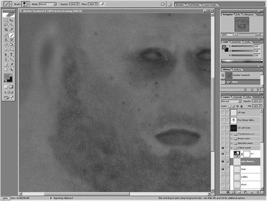
Figure 5-108
While the shading made the surface react correctly to light, the textures we create simply use those same shading values as a base from which to add details to the surface to make them more realistic.
To ensure that your textures do not change the overall shading values that you have assigned to the surface, and instead add only details and variations to them, you need to start them off by using the same values as a beginning.
This is actually quite simple. For example, let’s say you are shading a face and you have assigned a value of 32% Specularity to the surface. Of course as we know, skin has a lot of variation in its specularity, so ideally we’d paint a texture for this particular surface attribute so that we can add in variations and details where we want them. We know that overall we want a value of 32% Specularity with variations here and there. The best way to ensure that your painted texture does not alter this overall value is simply to start off your specular texture image using a gray value of 32% Brightness. This ensures that when the texture is applied to the model, the basic overall 32% Specularity value will remain unchanged, and the variations that you add to the texture image will be correct.
To do this, simply open your Color Picker in Photoshop (or whichever paint program you are using), and select a gray tone from the color palette on the left side of the window. Now look to the right side of the window and take note of the hue, saturation, and brightness (HSB) values. The brightness value is the one we need to fine-tune. For this example, we would simply enter a value of 32% as shown in Figure 5-109.
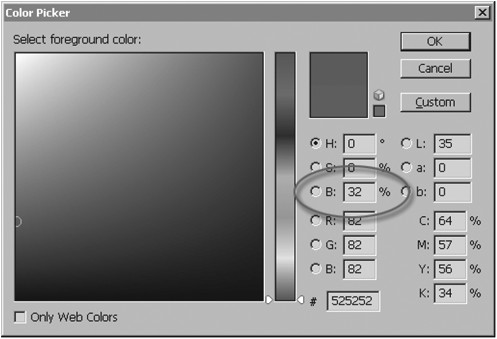
Figure 5-109
So as you can see, ensuring accuracy from LightWave shading values to Photoshop painting is really simple! All we need to do now is begin to make our specular texture with a flat value of this particular shade of gray and we won’t alter the overall shading value. The same concept applies to any of the surface attributes that are best created using shades of gray (which are basically all the surface properties with the exception of color).
Once we have created our texture maps, we then simply apply them to our surfaces, and render. If you have been meticulous in ensuring that everything will work correctly, you should get no surprises with the final result.

Figure 5-110