
Clustering algorithms can be categorized in different ways based on the techniques, the outputs, the process, and other considerations. In this topic, we will present some of the most widely used clustering algorithms.
There is a rich set of clustering techniques in use today for a wide variety of applications. This section presents some of them, explaining how they work, what kind of data they can be used with, and what their advantages and drawbacks are. These include algorithms that are prototype-based, density-based, probabilistic partition-based, hierarchy-based, graph-theory-based, and those based on neural networks.
k-means is a centroid- or prototype-based iterative algorithm that employs partitioning and relocation methods (References [10]). k-means finds clusters of spherical shape depending on the distance metric used, as in the case of Euclidean distance.
k-means can handle mostly numeric features. Many tools provide categorical to numeric transformations, but having a large number of categoricals in the computation can lead to non-optimal clusters. User-defined k, the number of clusters to be found, and the distance metric to use for computing closeness are two basic inputs. k-means generates clusters, association of data to each cluster, and centroids of clusters as the output.
The most common variant known as Lloyd's algorithm initializes k centroids for the given dataset by picking data elements randomly from the set. It assigns each data element to the centroid it is closest to, using some distance metric such as Euclidean distance. It then computes the mean of the data points for each cluster to form the new centroid and the process is repeated until either the maximum number of iterations is reached or there is no change in the centroids.
Mathematically, each step of the clustering can be seen as an optimization step where the equation to optimize is given by:

Here, ci is all points belong to cluster i. The problem of minimizing is classified as NP-hard and hence k-Means has a tendency to get stuck in local optimum.
- The choice of the number of clusters, k, is difficult to pick, but normally search techniques such as varying k for different values and measuring metrics such as sum of square errors can be used to find a good threshold. For smaller datasets, hierarchical k-Means can be tried.
- k-means can converge faster than most algorithms for smaller values of k and can find effective global clusters.
- k-means convergence can be affected by initialization of the centroids and hence there are many variants to perform random restarts with different seeds and so on.
- k-means can perform badly when there are outliers and noisy data points. Using robust techniques such as medians instead of means, k-Medoids, overcomes this to a certain extent.
- k-means does not find effective clusters when they are of arbitrary shapes or have different densities.
Density-based spatial clustering of applications with noise (DBSCAN) is a density-based partitioning algorithm. It separates dense region in the space from sparse regions (References [14]).
Only numeric features are used in DBSCAN. The user-defined parameters are MinPts and the neighborhood factor given by ϵ.
The algorithm first finds the ϵ-neighborhood of every point p, given by ![]() . A high density region is identified as a region where the number of points in a ϵ-neighborhood is greater than or equal to the given MinPts; the point such a ϵ-neighborhood is defined around is called a core points. Points within the ϵ-neighborhood of a core point are said to be directly reachable. All core points that can in effect be reached by hopping from one directly reachable core point to another point directly reachable from the second point, and so on, are considered to be in the same cluster. Further, any point that has fewer than MinPts in its ϵ-neighborhood, but is directly reachable from a core point, belongs to the same cluster as the core point. These points at the edge of a cluster are called border points. A noise point is any point that is neither a core point nor a border point.
. A high density region is identified as a region where the number of points in a ϵ-neighborhood is greater than or equal to the given MinPts; the point such a ϵ-neighborhood is defined around is called a core points. Points within the ϵ-neighborhood of a core point are said to be directly reachable. All core points that can in effect be reached by hopping from one directly reachable core point to another point directly reachable from the second point, and so on, are considered to be in the same cluster. Further, any point that has fewer than MinPts in its ϵ-neighborhood, but is directly reachable from a core point, belongs to the same cluster as the core point. These points at the edge of a cluster are called border points. A noise point is any point that is neither a core point nor a border point.
- The DBSCAN algorithm does not require the number of clusters to be specified and can find it automatically from the data.
- DBSCAN can find clusters of various shapes and sizes.
- DBSCAN has in-built robustness to noise and can find outliers from the datasets.
- DBSCAN is not completely deterministic in its identification of the points and its categorization into border or core depends on the order of data processed.
- Distance metrics selected such as Euclidean distance can often affect performance due to the curse of dimensionality.
- When there are clusters with large variations in the densities, the static choice of {MinPts, ϵ} can pose a big limitation.
Mean shift is a very effective clustering algorithm in many image, video, and motion detection based datasets (References [11]).
Only numeric features are accepted as data input in the mean shift algorithm. The choice of kernel and the bandwidth of the kernel are user-driven choices that affect the performance. Mean shift generates modes of data points and clusters data around the modes.
Mean shift is based on the statistical concept of kernel density estimation (KDE), which is a probabilistic method to estimate the underlying data distribution from the sample.
A kernel density estimate for kernel K (x) of given bandwidth h is given by:

For n points with dimensionality d. The mean shift algorithm works by moving each data point in the direction of local increasing density. To estimate this direction, gradient is applied to the KDE and the gradient takes the form of:


Here g(x)= –K'(x) is the derivative of the kernel. The vector, m(x), is called the mean shift vector and it is used to move the points in the direction
x(t+1) = xt + m(x)
Also, it is guaranteed to converge when the gradient of the density function is zero. Points that end up in a similar location are marked as clusters belonging to the same region.
- Mean shift is non-parametric and makes no underlying assumption on the data distribution.
- It can find non-complex clusters of varying shapes and sizes.
- There is no need to explicitly give the number of clusters; the choice of the bandwidth parameter, which is used in estimation, implicitly controls the clusters.
- Mean shift has no local optima for a given bandwidth parameter and hence it is deterministic.
- Mean shift is robust to outliers and noisy points because of KDE.
- The mean shift algorithm is computationally slow and does not scale well with large datasets.
- Bandwidth selection should be done judiciously; otherwise it can result in merged modes, or the appearance of extra, shallow modes.
GMM or EM is a probabilistic partition-based method that partitions data into k clusters using probability distribution-based techniques (References [13]).
Only numeric features are allowed in EM/GMM. The model parameter is the number of mixture components, given by k.
GMM is a generative method that assumes that there are k Gaussian components, each Gaussian component has a mean µi and covariance Ʃi. The following expression represents the probability of the dataset given the k Gaussian components:
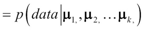


The two-step task of finding the means {µ1, µ2, …µk} for each of the k Gaussian components such that the data points assigned to each maximizes the probability of that component is done using the Expectation Maximization (EM) process.
The iterative process can be defined into an E-step, that computes the expected cluster for all data points for the cluster, in an iteration i:

The M-step maximizes to compute µt+1 given the data points belonging to the cluster:

The EM process can result in GMM convergence into local optimum.
- Works very well with any features; for categorical data, discrete probability is calculated, while for numeric a continuous probability function is estimated.
- It has computational scalability problems. It can result in local optimum.
- The value of k Gaussians has to be given apriori, similar to k-Means.
Hierarchical clustering is a connectivity-based method of clustering that is widely used to analyze and explore the data more than it is used as a clustering technique (References [12]). The idea is to iteratively build binary trees either from top or bottom, such that similar points are grouped together. Each level of the tree provides interesting summarization of the data.
Hierarchical clustering generally works on similarity-based transformations and so both categorical and continuous data are accepted. Hierarchical clustering only needs the similarity or distance metric to compute similarity and does not need the number of clusters like in k-means or GMM.
There are many variants of hierarchical clustering, but we will discuss agglomerative clustering. Agglomerative clustering works by first putting all the data elements in their own groups. It then iteratively merges the groups based on the similarity metric used until there is a single group. Each level of the tree or groupings provides unique segmentation of the data and it is up to the analyst to choose the right level that fits the problem domain. Agglomerative clustering is normally visualized using a dendrogram plot, which shows merging of data points at similarity. The popular choices of similarity methods used are:


- Hierarchical clustering imposes a hierarchical structure on the data even when there may not be such a structure present.
- The choice of similarity metrics can result in a vastly different set of merges and dendrogram plots, so it has a large dependency on user input.
- Hierarchical clustering suffers from scalability with increased data points. Based on the distance metrics used, it can be sensitive to noise and outliers.
SOM is a neural network based method that can be viewed as dimensionality reduction, manifold learning, or clustering technique (References [17]). Neurobiological studies show that our brains map different functions to different areas, known as topographic maps, which form the basis of this technique.
Only numeric features are used in SOM. Model parameters consists of distance function, (generally Euclidean distance is used) and the lattice parameters in terms of width and height or number of cells in the lattice.
SOM, also known as Kohonen networks, can be thought of as a two-layer neural network where each output layer is a two-dimensional lattice, arranged in rows and columns and each neuron is fully connected to the input layer.
Like neural networks, the weights are initially generated using random values. The process has three distinct training phases:
- Competitive phase: Neurons in this phase compete based on the discriminant values, generally based on distance between neuron weight and input vector; such that the minimal distance between the two decides which neuron the input gets assigned to. Using Euclidean distance, the distance between an input xi and neuron in the lattice position (j, i) is given by wji:

- Cooperation phase: In this phase, the winning neurons find the best spatial location in the topological neighborhood. The topological neighborhood for the winning neuron I(x) for a given neuron (j, i), at a distance Sij, neighborhood of size σ, is defined by:

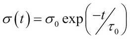
The neighborhood size is defined in the way that it decreases with time using some well-known decay functions such as an exponential, function defined as follows:
- Adaptive phase: In this phase, the weights of the winning neuron and its neighborhood neurons are updated. The update to weights is generally done using:

Here, the learning rate n(t) is again defined as exponential decay like the neighborhood size.
SOM Visualization using Unified Distance Matrix (U-Matrix) creates a single metric of average distance between the weights of the neuron and its neighbors, which then can be visualized in different color intensities. This helps to identify similar neurons in the neighborhood.
- The biggest advantage of SOM is that it is easy to understand and clustering of the data in two dimensions with U-matrix visualization enables understanding the patterns very effectively.
- Choice of similarity/distance function makes vast difference in clusters and must be carefully chosen by the user.
- SOM's computational complexity makes it impossible to use on datasets greater than few thousands in size.
Spectral clustering is a partition-based clustering technique using graph theory as its basis (References [15]). It converts the dataset into a connected graph and does graph partitioning to find the clusters. This is a popular method in image processing, motion detection, and some unstructured data-based domains.
Only numeric features are used in spectral clustering. Model parameters such as the choice of kernel, the kernel parameters, the number of eigenvalues to select, and partitioning algorithms such as k-Means must be correctly defined for optimum performance.
The following steps describe how the technique is used in practice:
- Given the data points, an affinity (or adjacency) matrix is computed using a smooth kernel function such as the Gaussian kernel:For the points that are closer,

 and for points further away,
- The next step is to compute the graph Laplacian matrix using various methods of normalizations. All Laplacian matrix methods use the diagonal degree matrix D, which measures degree at each node in the graph:

A simple Laplacian matrix is L = D (degree matrix) – A(affinity matrix).
- Compute the first k eigenvalues from the eigenvalue problem or the generalized eigenvalue problem.
- Use a partition algorithm such as k-Means to further separate clusters in the k-dimensional subspace.
- Spectral clustering works very well when the cluster shape or size is irregular and non-convex. Spectral clustering has too many parameter choices and tuning to get good results is quite an involved task.
- Spectral clustering has been shown, theoretically, to be more stable in the presence of noisy data. Spectral clustering has good performance when the clusters are not well separated.
Affinity propagation can be viewed as an extension of K-medoids method for its similarity with picking exemplars from the data (References [16]). Affinity propagation uses graphs with distance or the similarity matrix and picks all examples in the training data as exemplars. Iterative message passing as affinities between data points automatically detects clusters, the exemplars, and even the number of clusters.
Typically, other than maximum number of iterations, which is common to most algorithms, no input parameters are required.
Two kinds of messages are exchanged between the data points that we will explain first:
-
Responsibility r(i,k): This is a message from the data point to the candidate exemplar. This gives a metric of how well the exemplar is suited for that data point compared to other exemplars. The rules for updating the responsibility are as follows:
 where
s(i, k) = similarity between two data points i and k.
where
s(i, k) = similarity between two data points i and k.a(i, k) = availability of exemplar k for i.
- Availability a(i,k): This is a message from the candidate exemplar to a data point. This gives a metric indicating how good of a support the exemplar can be to the data point, considering other data points in the calculations. This can be viewed as soft cluster assignment. The rule for updating the availability is as follows:


Figure 4: Message types used in Affinity Propagation
The algorithm can be summed up as follows:
- Affinity propagation is a deterministic algorithm. Both k-means or K-medoids are sensitive to the selection of initial points, which is overcome by considering every point as an exemplar.
- The number of clusters doesn't have to be specified and is automatically determined through the process.
- It works in non-metric spaces and doesn't require distances/similarity to even have constraining properties such as triangle inequality or symmetry. This makes the algorithm usable on a wide variety of datasets with categorical and text data and so on:
- The algorithm can be parallelized easily due to its update methods and it has fast training time.
Clustering validation and evaluation is one of the most important mechanisms to determine the usefulness of the algorithms (References [18]). These topics can be broadly classified into two categories:
Internal evaluation uses only the clusters and data information to gather metrics about how good the clustering results are. The applications may have some influence over the choice of the measures. Some algorithms are biased towards particular evaluation metrics. So care must be taken in choosing the right metrics, algorithms, and parameters based on these considerations. Internal evaluation measures are based on different qualities, as mentioned here:
Here's a compact explanation of the notation used in what follows: dataset with all data elements =D, number of data elements =n, dimensions or features of each data element=d, center of entire data D = c, number of clusters = NC, ith cluster = Ci, number of data in the ith cluster =ni, center of ith cluster = ci, variance in the ith cluster = σ(Ci), distance between two points x and y = d (x,y).
The goal is to measure the degree of difference between clusters using the ratio of the sum of squares between clusters to the total sum of squares on the whole data. The formula is given as follows:

The goal is to identify dense and well-separated clusters. The measure is given by maximal values obtained from the following formula:


The external evaluation measures of clustering have similarity to classification metrics using elements from the confusion matrix or using information theoretic metrics from the data and labels. Some of the most commonly used measures are as follows.
Rand index measures the correct decisions made by the clustering algorithm using the following formula:

F-Measure combines the precision and recall measures applied to clustering as given in the following formula:


Here, nij is the number of data elements of class i in the cluster j, nj is the number of data in the cluster j and ni is the number of data in the class i. The higher the F-Measure, the better the clustering quality.
NMI is one of the many entropy-based measures applied to clustering. The entropy associated with a clustering C is a measure of the uncertainty about a cluster picking a data element randomly.
![]() where
where  is the probability of the element getting picked in cluster Ci.
Mutual information between two clusters is given by:

Here  , which is the probability of the element being picked by both clusters C and C'.
Normalized mutual information (NMI) has many forms; one is given by:
