
Generally, all Probabilistic Graphical Models have three basic elements that form the important sections:
- Representation: This answers the question of what does the model mean or represent. The idea is how to represent and store the probability distribution of P(X1, X2, …. Xn).
- Inference: This answers the question: given the model, how do we perform queries and get answers. This gives us the ability to infer the values of the unknown from the known evidence given the structure of the models. Motivating the main discussion points are various forms of inferences involving trade-offs between computational and correctness concerns.
- Learning: This answers the question of what model is right given the data. Learning is divided into two main parts:
- Learning the parameters given the structure and data
- Learning the structure with parameters given the data
We will use the well-known student network as an example of a Bayesian network in our discussions to illustrate the concepts and theory. The student network has five random variables capturing the relationship between various attributes defined as follows:
- Difficulty of the exam (D)
- Intelligence of the student (I)
- Grade the student gets (G)
- SAT score of the student (S)
- Recommendation Letter the student gets based on grade (L).
Each of these attributes has binary categorical values, for example, the variable Difficulty (D) has two categories (d0, d1) corresponding to low and high, respectively. Grades (G) has three categorical values corresponding to the grades (A, B, C). The arrows as indicated in the section on graphs indicate the dependencies encoded from the domain knowledge—for example, Grade can be determined given that we know the Difficulty of the exam and Intelligence of the student while the Recommendation Letter is completely determined if we know just the Grade (Figure 2). It can be further observed that no explicit edge between the variables indicates that they are independent of each other—for example, the Difficulty of the exam and Intelligence of the student are independent variables.

Figure 2. The "Student" network
A graph compactly represents the complex relationships between random variables, allowing fast algorithms to make queries where a full enumeration would be prohibitive. In the concepts defined here, we show how directed acyclic graph structures and conditional independence make problems involving large numbers of variables tractable.
A Bayesian network is defined as a model of a system with:
- A number of random variables {X1, X2, …. Xk}
- A Directed Acyclic Graph (DAG) with nodes representing random variables.
- A local conditional probability distribution (CPD) for each node with dependence to its parent nodes P(Xi | parent(Xi)).
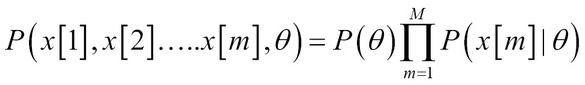
- A joint probability distribution obtained using the chain rule of distribution is a factor given as:

- For the student network defined, the joint distribution capturing all nodes can be represented as:
P(D,I,G,S,L)=P(D)P(I)P(G¦D,I)P(S¦I)P(L¦G)
The Bayesian networks help in answering various queries given some data and facts, and these reasoning patterns are discussed here.
If evidence is given as, for example, "low intelligence", then what would be the chances of getting a "good letter" as shown in Figure 3, in the top right quadrant? This is addressed by causal reasoning. As shown in the first quadrant, causal reasoning flows from the top down.
If evidence such as a "bad letter" is given, what would be the chances that the student got a "good grade"? This question, as shown in Figure 3 in the top left quadrant, is addressed by evidential reasoning. As shown in the second quadrant, evidential reasoning flows from the bottom up.
Obtaining interesting patterns from finding a "related cause" is the objective of intercausal reasoning. If evidence of "grade C" and "high intelligence" is given, then what would be the chance of course difficulty being "high"? This type of reasoning is also called "explaining away" as one cause explains the reason for another cause and this is illustrated in the third quadrant, in the bottom-left of Figure 3.
If a student takes an "easy" course and has a "bad letter", what would be the chances of him getting a "grade C" ? This is explained by queries with combined reasoning patterns. Note that it has mixed information and does not a flow in a single fixed direction as in the case of other reasoning patterns and is shown in the bottom-right of the figure, in quadrant 4:

Figure 3. Reasoning patterns
The conditional independencies between the nodes can be exploited to reduce the computations when performing queries. In this section, we will discuss some of the important concepts that are associated with independencies.
Influence is the effect of how the condition or outcome of one variable changes the value or the belief associated with another variable. We have seen this from the reasoning patterns that influence flows from variables in direct relationships (parent/child), causal/evidential (parent and child with intermediates) and in combined structures.
The only case where the influence doesn't flow is when there is a "v-structure". That is, given edges between three variables ![]() there is a v-structure and no influence flows between Xi - 1 and Xi + 1. For example, no influence flows between the Difficulty of the course and the Intelligence of the student.
there is a v-structure and no influence flows between Xi - 1 and Xi + 1. For example, no influence flows between the Difficulty of the course and the Intelligence of the student.
Random variables X and Y are said to be d-separated in the graph G, given there is no active trail between X and Y in G given Z. It is formally denoted by:
dsepG (X,Y|Z)
The point of d-separation is that it maps perfectly to the conditional independence between the points. This gives to an interesting property that in a Bayesian network any variable is independent of its non-descendants given the parents of the node.
In the Student network example, the node/variable Letter is d-separated from Difficulty, Intelligence, and SAT given the grade.
From the d-separation, in graph G, we can collect all the independencies from the d-separations and these independencies are formally represented as:

If P satisfies I(G) then we say the G is an independency-map or I-Map of P.
The main point of I-Map is it can be formally proven that a factorization relationship to the independency holds. The converse can also be proved.
In simple terms, one can read in the Bayesian network graph G, all the independencies that hold in the distribution P regardless of any parameters!
Consider the student network—its whole distribution can be shown as:
P(D,I,G,S,L) = P(D)P(I|D)P(G¦D,I)P(S¦D,I,G)P(L¦D,I,G,S)
Now, consider the independence from I-Maps:
- Variables I and D are non-descendants and not conditional on parents so P(I|D) = P(I)
- Variable S is independent of its non-descendants D and G, given its parent I. P(S¦D,I,G)=P(S|I)
- Variable L is independent of its non-descendants D, I, and S, given its parent G. P(L¦D,I,G,S)=P(L|G)
(D,I,G,S,L)=P(D)P(I)P(G¦D,I)P(S¦I)P(L¦G)
Thus, we have shown that I-Map helps in factorization given just the graph network!
The biggest advantage of probabilistic graph models is their ability to answer probability queries in the form of conditional or MAP or marginal MAP, given some evidence.
Formally, the probability of evidence E = e is given by:

But the problem has been shown to be NP-Hard (Reference [3]) or specifically, #P-complete. This means that it is intractable when there are a large number of trees or variables. Even for a tree-width (number of variables in the largest clique) of 25, the problem seems to be intractable—most real-world models have tree-widths larger than this.
So if the exact inference discussed before is intractable, can some approximations be used so that within some bounds of the error, we can make the problem tractable? It has been shown that even an approximate algorithm to compute inferences with an error ? < 0.5, so that we find a number p such that |P(E = e) – p|< ?, is also NP-Hard.
But the good news is that this is among the "worst case" results that show exponential time complexity. In the "general case" there can be heuristics applied to reduce the computation time both for exact and approximate algorithms.
Some of the well-known techniques for performing exact and approximate inferencing are depicted in Figure 4, which covers most probabilistic graph models in addition to Bayesian networks.

Figure 4. Exact and approximate inference techniques
It is beyond the scope of this chapter to discuss each of these in detail. We will explain a few of the algorithms in some detail accompanied by references to give the reader a better understanding.
Here we will describe two techniques, the variable elimination algorithm and the clique-tree or junction-tree algorithm.
The basics of the Variable elimination (VE) algorithm lie in the distributive property as shown:
(ab+ac+ad)= a (b+c+d)
In other words, five arithmetic operations of three multiplications and two additions can be reduced to four arithmetic operations of one multiplication and three additions by taking a common factor a out.
Let us understand the reduction of the computations by taking a simple example in the student network. If we have to compute a probability query such as the difficulty of the exam given the letter was good, that is, P(D¦L=good)=?.
Using Bayes theorem:
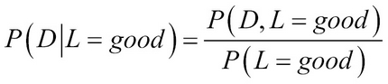
To compute P(D¦L=good)=? we can use the chain rule and joint probability:

If we rearrange the terms on the right-hand side:

If we now replace ![]() since the factor is independent of the variable I that S is conditioned on, we get:
since the factor is independent of the variable I that S is conditioned on, we get:

Thus, if we proceed carefully, eliminating one variable at a time, we have effectively converted O(2n) factors to O(nk2) factors where n is the number of variables and k is the number of observed values for each.
Thus, the main idea of the VE algorithm is to impose an order on the variables such that the query variable comes last. A list of factors is maintained over the ordered list of variables and summation is performed. Generally, we use dynamic programming in the implementation of the VE algorithm (References [4]).
Inputs:
Output:
- P(Q|E = e)
The algorithm calls the eliminate function in a loop, as shown here:
VariableElimination:
- While ?, the set of all random variables in the Bayesian network is not empty
- Remove the first variable Z from ?
- eliminate(F, Z)
- end loop.
- Set ? product of all factors in F
- Instantiate observed variables in ? to their observed values.
-
return
 (renormalization)
eliminate (F, Z)
- Remove from the F all functions, for example, X1, X2, …. Xk that involve Z.
-
Compute new function

-
Compute new function

- Add new function ? to F
- Return F
Consider the same example of the student network with P(D, L = good) as the goal.
- Pick a variable ordering list: S, I, L, G, and D
- Initialize the active factor list and introduce the evidence:
List: P(S¦I)P(I)P(D)P(G¦I,D)P(L¦G)d(L = good)
- Eliminate the variable SAT or S off the list

List: P(I)P(D)P(G¦I,D)P(L¦G)d(L = good) ?1 (I)
- Eliminate the variable Intelligence or I

List: P(D)P(L¦G)d(L = good) ?2 (G,D)
- Eliminate the variable Letter or L

List: P(D) ?3 (G) ?2 (G,D)
- Eliminate the variable Grade or G

List: P(D) ?4 (D)
Thus with two values, P(D=high) ?4 (D=high) and P(D=low) ?4 (D=low), we get the answer.
The advantages and limitations are as follows:
- The main advantage of the VE algorithm is its simplicity and generality that can be applied to many networks.
- The computational reduction advantage of VE seems to go away when there are many connections in the network.
- The choice of optimal ordering of variables is very important for the computational benefit.
Junction tree or Clique Trees are more efficient forms of variable elimination-based techniques.
Inputs:
Output:
- P(Q|E = e)
The steps involved are as follows:
- Moralization: This is a process of converting a directed graph into an undirected graph with the following two steps:
- Replace directed edges with undirected edges between the nodes.
- If there are two nodes or vertices that are not connected but have a common child, add an edge connecting them. (Note the edge between V4 and V5 and V2 and V3 in Figure 5):
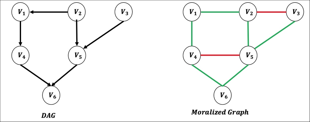
Figure 5. Graph moralization of DAG showing in green how the directional edges are changed and red edges showing new additions.
- Triangulation: For understanding triangulation, chords must be formed. The chord of a cycle is a pair of vertices Vi and Vj of non-consecutive vertices that have an edge between them. A graph is called a chordal or triangulated graph if every cycle of length ≥ 4 has chords. Note the edge between V1 and V5 in Figure 6 forming chords to make the moralized graph a chordal/triangulated graph:

Figure 6. Graph triangulation with blue edge addition to convert a moralized graph to a chordal graph.
- Junction Tree: From the chordal graphs a junction tree is formed using the following steps:
- Find all the cliques in the graph and make them nodes with the cluster of all vertices. A clique is a subgraph where an edge exists between each pair of nodes. If two nodes have one or more common vertices create an edge consisting of the intersecting vertices as a separator or sepset. For example, the cycle with edges V1, V4, V5 and V6, V4, V5 that have a common edge between V4, V5 can be reduced to a clique as shown with the common edge as separator.
If the preceding graph contains a cycle, all separators in the cycle contain the same variable. Remove the cycle in the graph by creating a minimum spanning tree, while including maximum separators. The entire transformation process is shown in Figure 7:

Figure 7. Formation of a Junction Tree
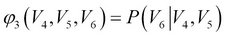
- Run the Message Passing algorithm on Junction Tree: Junction tree can be used to compute the joint distribution using factorization of cliques and separators as

- Compute the parameters of Junction Tree: The junction tree parameters can be obtained per node using the parent nodes in the original Bayesian network and are called clique potentials, as shown here:
- (?1 (V2,V3,V5) = P(V5 |V2,V3)P(V3)(Note in the original Bayesian network edge V5 is dependent on V2, V3, whereas V3 is independent)


- Message Passing between nodes/cliques in Junction Tree: A node in the junction tree, represented by clique Ci, multiplies all incoming messages from its neighbors with its own clique potential, resulting in a factor
 whose scope is the clique. It then sums out all the variables except the ones on sepset or separators Si,j between Ci and Cj and then sends the resulting factor as a message to Cj.
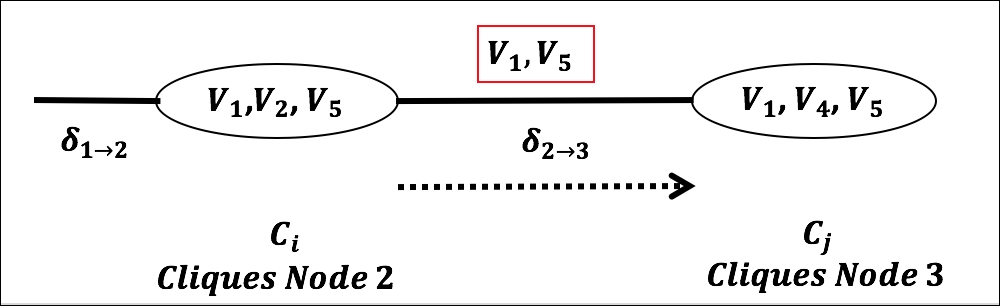
Figure 8. Message passing between nodes/cliques in Junction Tree

Thus, when the message passing reaches the tree root, the joint probability distribution is completed.
Here we discuss belief propagation, a commonly used message passing algorithm for doing inference by introducing factor graphs and the messages that can flow in these graphs.
Belief propagation is one of the most practical inference techniques that has applicability across most probabilistic graph models including directed, undirected, chain-based, and temporal graphs. To understand the belief propagation algorithm, we need to first define factor graphs.
We know from basic probability theory that the entire joint distribution can be represented as a factor over a subset of variables as

In DAG or Bayesian networks fs(Xs) is a conditional distribution. Thus, there is a great advantage in expressing the joint distribution over factors over the subset of variables.
Factor graph is a representation of the network where the variables and the factors involving the variables are both made into explicit nodes (References [11]). In a simplified student network from the previous section, the factor graph is shown in Figure 9.

Figure 9. Factor graph of simplified "Student" network
A factor graph is a bipartite graph, that is, it has two types of nodes, variables and factors.
The edges flow between two opposite types, that is, from variables to factors and vice versa.
Converting the Bayesian network to a factor graph is a straightforward procedure as shown previously where you start adding variable nodes and conditional probability distributions as factor nodes. The relationship between the Bayesian network and factor graphs is one-to-many, that is, the same Bayesian network can be represented in many factor graphs and is not unique.
There are two distinct messages that flow in these factor graphs that form the bulk of all computations through communication.
- Message from factor nodes to variable nodes: The message that is sent from a factor node to the variable node can be mathematically represented as follows:


 where
where  Thus,
Thus,  is the message from factor node fs to x and the product of all such messages from neighbors of x to x gives the combined probability to x:
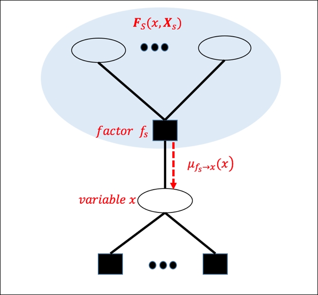
Figure 10. Message-passing from factor node to variable node
- Message from variable nodes to factor nodes: Similar to the previous example, messages from variable to factor can be shown to be


Thus, all the factors coming to the node xm are multiplied except for the factor it is sending to.

Figure 11. Message-passing from variable node to factor node
Inputs:
Output:
- P(Q|E = e)
- Create a factor graph from the Bayesian network as discussed previously.
- View the node Q as the root of the graph.
-
Initialize all the leaf nodes, that is:
 and
and

- Apply message passing from a leaf to the next node in a recursive manner.
- Move to the next node, until root is reached.
- Marginal at the root node gives the result.
The advantages and limitaions are as follows:
We will discuss a simple approach using particles and sampling to illustrate the process of generating the distribution P(X) from the random variables. The idea is to repeatedly sample from the Bayesian network and use the samples with counts to approximate the inferences.
The key idea is to generate i.i.d. samples iterating over the variables using a topological order. In case of some evidence, for example, P(X|E = e) that contradicts the sample generated, the easiest way is to reject the sample and proceed.
Inputs:
- List of Condition Probability Distribution/Table F
- List of query variables Q
- List of observed variables E and the observed value e
Output:
- P(Q|E = e)
- For j = 1 to m //number of samples
- Create a topological order of variables, say X1, X2, … Xn.
- For i = 1 to n
- ui ? X(parent(Xi)) //assign parent(Xi) to variables
- sample(xi, P(Xi | ui) //sample Xi given parent assignments
- if(xi ?, P(Xi | E = e) reject and go to 1.1.2. //reject sample if it doesn't agree with the evidence.
- Return (X1, X2,….Xn) as sample.
- Compute P(Q | E = e) using counts from the samples.
An example of one sample generated for the student network can be by sampling Difficulty and getting Low, next, sampling Intelligence and getting High, next, sampling grade using the CPD table for Difficulty=low and Intelligence=High and getting Grade=A, sampling SAT using CPD for Intelligence=High and getting SAT=good and finally, using Grade=A to sample from Letter and getting Letter=Good. Thus, we get first sample (Difficulty=low, Intelligence=High, Grade=A, SAT=good, Letter=Good)
The idea behind learning is to generate either a structure or find parameters or both, given the data and the domain experts.
The goals of learning are as follows:
- To facilitate inference in Bayesian networks. The pre-requisite of inferencing is that the structure and parameters are known, which are the output of learning.
- To facilitate prediction using Bayesian networks. Given observed variables X, predict the target variables Y.
- To facilitate knowledge discovery using Bayesian networks. This means understanding causality, relationships, and other features from the data.
Learning, in general, can be characterized by Figure 12. The assumption is that there is a known probability distribution P* that may or may not have been generated from a Bayesian network G*. The observed data samples are assumed to be generated or sampled from that known probability distribution P*. The domain expert may or may not be present to include the knowledge or prior beliefs about the structure. Bayesian networks are one of the few techniques where domain experts' inputs in terms of relationships in variables or prior probabilities can be used directly, in contrast to other machine learning algorithms. At the end of the process of knowledge elicitation and learning from data, we get as an output a Bayesian network with defined structure and parameters (CPTs).

Figure 12. Elements of learning with Bayesian networks
Based on data quality (missing data or complete data) and knowledge of structure from the expert (unknown and known), the following are four classes that Learning in Bayesian networks fall into, as shown in Table 2:
Table 2. Classes of Bayesian network learning
In this section, we will discuss two broadly used methodologies to estimate parameters given the structure. We will discuss only with the complete data and readers can refer to the discussion in (References [8]) for incomplete data parameter estimation.
Maximum
likelihood estimation (MLE) is a very generic method and it can be defined as: given a data set D, choose parameters ![]() that satisfy:
that satisfy:

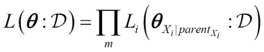
Maximum likelihood is the technique of choosing parameters of the Bayesian network given the training data. For a detailed discussion, see (References [6]).
Given the known Bayesian network structure of graph G and training data ![]() , we want to learn the parameters or CPDs—or CPTs to be precise. This can be formulated as:
, we want to learn the parameters or CPDs—or CPTs to be precise. This can be formulated as:

Now each example or instance ![]() can be written in terms of variables. If there are i variables represented by xi and the parents of each is given by parentXi then:
can be written in terms of variables. If there are i variables represented by xi and the parents of each is given by parentXi then:

Interchanging the variables and instances:

The term is:

This is the conditional likelihood of a particular variable x
i given its parents parentXi. Thus, parameters for these conditional likelihoods are a subset of parameters given by ![]() . Thus:
. Thus:
Here, ![]() is called the local likelihood function. This becomes very important as the total likelihood decomposes into independent terms of local likelihood and is known as the global decomposition property of the likelihood function. The idea is that these local likelihood functions can be further decomposed for a tabular CPD by simply using the count of different outcomes from the training data.
is called the local likelihood function. This becomes very important as the total likelihood decomposes into independent terms of local likelihood and is known as the global decomposition property of the likelihood function. The idea is that these local likelihood functions can be further decomposed for a tabular CPD by simply using the count of different outcomes from the training data.
Let Nijk be the number of times we observe variable or node i in the state k, given the parent node configuration j:
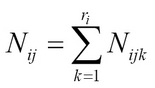
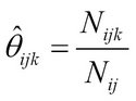
For example, we can have a simple entry corresponding to Xi = a and parentXi = b by estimating the likelihood function from the training data as:

Consider two cases, as an example. In the first, ![]() is satisfied by 10 instances with parentXi = b =100. In the second,
is satisfied by 10 instances with parentXi = b =100. In the second, ![]() is satisfied by 100 when parentXi = b =1000. Notice both probabilities come to the same value, whereas the second has 10 times more data and is the "more likely" estimate! Similarly, familiarity with domain or prior knowledge, or lack of it due to uncertainty, is not captured by MLE. Thus, when the number of samples are limited or when the domain experts are aware of the priors, then this method suffers from serious issues.
is satisfied by 100 when parentXi = b =1000. Notice both probabilities come to the same value, whereas the second has 10 times more data and is the "more likely" estimate! Similarly, familiarity with domain or prior knowledge, or lack of it due to uncertainty, is not captured by MLE. Thus, when the number of samples are limited or when the domain experts are aware of the priors, then this method suffers from serious issues.
This technique overcomes the issue of MLE by encoding prior knowledge about the parameter ? with a probability distribution. Thus, we can encode our beliefs or prior knowledge about the parameter space as a probability distribution and then the joint distribution of variables and parameters are used in estimation.
Let us consider single variable parameter learning where we have instances x[1], x[2] … x[M] and they all have parameter ?X.

Figure 13. Single variable parameter learning

Thus, the network is a joint probability model over parameters and data. The advantage is we can use it for the posterior distribution:
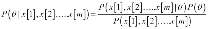
, P(?) = prior,
![]() Thus, the difference between the maximum likelihood and Bayesian estimation is the use of the priors.
Thus, the difference between the maximum likelihood and Bayesian estimation is the use of the priors.
Generalizing it to a Bayesian network G given the dataset D:


If we assume global independence of parameters

Thus, we get
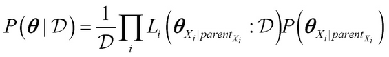
Again, as before, subset ?Xi | parentXi of ? is local and thus the entire posterior can be computed in local terms!
Often, in practice, a continuous probability distribution known as Dirichlet distribution—which is a Beta distribution—is used to represent priors over the parameters.

Probability Density Function:

Here, ![]() ,
, ![]() The alpha terms are known as hyperparameters and aijri > 0. The
The alpha terms are known as hyperparameters and aijri > 0. The ![]() is the pseudo count, also known as equivalent sample size and it gives us a measure of the prior.
is the pseudo count, also known as equivalent sample size and it gives us a measure of the prior.
The Beta function, B(aij) is normally expressed in terms of gamma function as follows

The advantage of using Dirichlet distribution is it is conjugate in nature, that is, irrespective of the likelihood, the posterior is also a Dirichlet if the prior is Dirichlet!
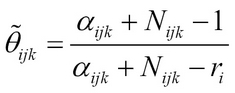
It can be shown that the posterior distribution for the parameters ?ijk is a Dirichlet with updated hyperparameters and has a closed form solution!
aijk = aijk + Nijk
If we use maximum a posteriori estimate and posterior means they can be shown to be:

Learning Bayesian network without any domain knowledge or understanding of structures includes learning the structure and the parameters. We will first discuss some measures that are used for evaluating the network structures and then discuss a few well-known algorithms for building optimal structures.
The measures used to evaluate a Bayes network structure, given the dataset, can be broadly divided into the following categories and details of many are available here (References [14]).
- Deviance-Threshold Measure: The two common techniques to measure deviance between two variables used in the network and structure are Pearson's chi-squared statistic and the Kullback-Leibler distance.
Given the dataset D of M samples, consider two variables Xi and Xj, the Pearson's chi-squared statistic measuring divergence is
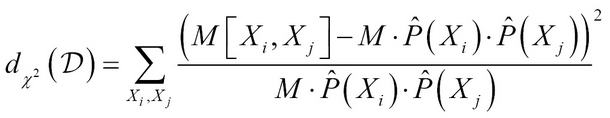


d?2(D) is 0; when the variables are independent and larger values indicate there is dependency between the variables.
Kullback-Leibler divergence is:

dI(D) is again 0, it shows independence and the larger values indicates dependency. Using various statistical hypothesis tests, a threshold can be used to determine the significance.
- Structure Score Measure: There are various measures to give scores to a structure in a Bayes network. We will discuss the most commonly used measures here. A log-likelihood score discussed in parameter learning can be used as a score for the structure:

- Bayesian information score (BIC) is also quite a popular scoring technique as it avoids overfitting by taking into consideration the penalty for complex structures, as shown in the following equation


The penalty function is logarithmic in M, so, as it increases, the penalty is less severe for complex structures.
The Akaike information score (AIC), similar to BIC, has similar penalty based scoring and is:

Bayesian scores discussed in parameter learning are also employed as scoring measures.
We will discuss a few algorithms that are used for learning structures in this section; details can be found here (References [15]).
Constraint-based algorithms use independence tests of various variables, trying to find different structural dependencies that we discussed in previous sections such as the d-separation, v-structure, and so on, by following the step-by-step process discussed here.
The input is the dataset D with all the variables {X,Y..} known for every instance {1,2, ... m}, and no missing values. The output is a Bayesian network graph G with all edges, directions known in E and the CPT table.
- Create an empty set of undirected edge E.
- Test for conditional independence between two variables independent of directions to have an edge.
- If for all subset S = U – {X, Y}, if X is independent of Y, then add it to the set of undirected edge E'.
- Once all potential undirected edges are identified, directionality of the edge is inferred from the set E'.
-
Considering a triplet {X, Y, Z}, if there is an edge X – Z and Y – Z, but no edge between X – Y using all variables in the set, and further, if X is not independent of Y given all the edges S = U – {X, Y, Z}, this implies the direction of
 and
and  .
.
-
Add the edges and to set E.
- Update the CPT table using local calculations.
-
Considering a triplet {X, Y, Z}, if there is an edge X – Z and Y – Z, but no edge between X – Y using all variables in the set, and further, if X is not independent of Y given all the edges S = U – {X, Y, Z}, this implies the direction of
- Return the Bayes network G, edges E, and the CPT tables.
- Lack of robustness is one of the biggest drawbacks of this method. A small error in data can cause a big impact on the structure due to the assumptions of independence that will creep into the individual independence tests.
- Scalability and computation time is a major concern as every subset of variables are tested and is approximately 2n. As the number of variables increase to the 100s, this method fails due to computation time.
The search and score method can be seen as a heuristic optimization method where iteratively, structure is changed through small perturbations, and measures such as BIC or MLE are used to give score to the structures to find the optimal score and structure. Hill climbing, depth-first search, genetic algorithms, and so on, have all been used to search and score.
Input is dataset D with all the variables {X,Y..} known for every instance {1,2, ... m} and no missing values. The output is a Bayesian network graph G with all edges and directions known in E.

Figure 14. Search and Score
- Initialize the Graph G, either based on domain knowledge or empty or full. Initialize the Edge set E based on the graph and initialize the CPT tables T based on the graph G, E, and the data D. Normally terminating conditions are also mentioned such as maxIterations:
- maxScore= -8, score=computeScore(G,E, T)
- Do
- maxScore=score
-
For each variable pair (X, Y)
-
For each

- New Graph G' based on parents and variables with edge changes.
- Compute new CPTs T' ? computeCPT(G',E',D).
- currentScore = computeScore(G',E',T')
- If currentScore > score:
- score = currentScore
- G' = G, E' = E
-
For each
-
Repeat 3 while (
