
In this section, we will cover some basic specialized probabilistic graph models that are very useful in different machine learning applications.
In Chapter 2, Practical Approach to Real-World Supervised Learning, we discussed the Naïve Bayes network, which makes the simplified assumption that all variables are independent of each other and only have dependency on the target or the class variable. This is the simplest Bayesian network derived or assumed from the dataset. As we saw in the previous sections, learning complex structures and parameters in Bayesian networks can be difficult or sometimes intractable. The tree augmented network or TAN (References [9]) can be considered somewhere in the middle, introducing constraints on how the trees are connected. TAN puts a constraint on features or variable relationships. A feature can have only one other feature as parent in addition to the target variable, as illustrated in the following figure:

Figure 17. Tree augmented network showing comparison with Naïve Bayes and Bayes network and the constraint of one parent per node.
Inputs are the training dataset D with all the features as variables {X, Y..}. The features have discrete outcomes, if they don't need to be discretized as a pre-processing step.
Outputs are TAN as Bayesian network with CPTs.
- Compute mutual information between every pair of variables from the training dataset.
- Build an undirected graph with each node being the variable and edge being the mutual information between them.
- Create a maximum weighted spanning tree.
- Transform the spanning tree to a directed graph by selecting the outcome or the target variable as the root and having all the edges flowing in the outwards direction.
- If there is no directed edge between the class variable and other features, add it.
- Compute the CPTs based on the DAG or TAN constructed previously.
Markov Chains are specialized probabilistic graph models, with directed graphs containing loops. Markov chains can be seen as extensions of automata where the weights are probabilities of transition. Markov chains are useful to model temporal or sequence of changes that are directly observable. See (References [12]) for further study.
Figure 17 represents a Markov chain (first order) and the general definition can be given as a stochastic process consisting of
Nodes as states, ![]() .
.
Edges representing transition probabilities between the states or nodes. It is generally represented as a matrix ![]() , which is a N X N matrix where N is the number of nodes or states. The value of
, which is a N X N matrix where N is the number of nodes or states. The value of ![]() captures the transition probability to node ql given the state qk. The rows of matrix add to 1 and the values of
captures the transition probability to node ql given the state qk. The rows of matrix add to 1 and the values of ![]() .
.
Initial probabilities of being in the state, p = {p1, p2, … pN}.
Thus, it can be written as a triple M= (Q, A, p) and the probability of being in any state only depends on the last state (first order):

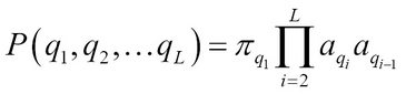

Figure 18. First-order Markov chain
In many real-world situations, the events we are interested in are not directly observable. For example, the words in sentences are observable, but the part-of-speech that generated the sentence is not. Hidden Markov models (HMM) help us in modeling such states where there are observable events and hidden states (References [13]). HMM are widely used in various modeling applications for speech recognition, language modeling, time series analysis, and bioinformatics applications such as DNA/protein sequence predictions, to name a few.

Figure 19. Hidden Markov model showing hidden variables and the observables.
Hidden Markov models can be defined again as a triple ![]() , where:
, where:
-
is a set of finite states or symbols that are observed.

-
Q is a set of finite states that are not observed
 .
.
- T are the parameters.
The state transition matrix, given as ![]() captures the probability of transition from state qk to ql.
captures the probability of transition from state qk to ql.
Emission probabilities capturing relationships between the hidden and observed state, given as ![]() and b ? ?.
and b ? ?. ![]() .
.
Initial state distribution p = {p1, p2, … pN}.
Thus, a path in HMM consisting of a sequence of hidden states Q = {q1, q2, … qL} is a first order Markov chain M= (Q, A, p). This path in HMM emits a sequence of symbols, x1, x2, xL, referred to as the observations. Thus, knowing both the observations and hidden states the joint probability is:

In real-world situations, we only know the observations x and do not know the hidden states q. HMM helps us to answer the following questions:
Let us assume the observations x = x1, x2, xL and we want to find the path ![]() that generated the observations. This can be given as:
that generated the observations. This can be given as:
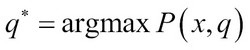
The path q* need not be unique, but for computation and explanation the assumption of the unique path is often made. In a naïve way, we can compute all possible paths of length L of q and chose the one(s) with the highest probability giving exponential computing terms or speed. More efficient is using Viterbi's algorithm using the concept of dynamic programming and recursion. It works on the simple principle of breaking the equation into simpler terms as:


Here, ![]() and
and ![]() Given the initial condition
Given the initial condition ![]() and using dynamic programming with keeping pointer to the path, we can efficiently compute the answer.
and using dynamic programming with keeping pointer to the path, we can efficiently compute the answer.
The probability of being in a state qi = k given the observation x can be written using Bayes theorem as:

The numerator can be rewritten as:


Where  is called a Forward variable and
 ![]() is called a Backward variable.
is called a Backward variable.
The computation of the forward variable is similar to Viterbi's algorithm using dynamic programming and recursion where summation is done instead:


The probability of observing x can be, then

The forward variable is the joint probability and the backward variable is a conditional probability:


It is called a backward variable as the dynamic programming table is filled starting with the Lth column to the first in a backward manner. The backward probabilities can also be used to compute the probability of observing x as:
