
22
Production Planning
22.1 Introduction
In the previous chapters, we examined the processes used to create products. But the creation of a product, especially a modern complex one comprising many elements, also necessitates careful planning and control of the production system. This section of the book considers how the resources of materials, machines, money and people, or manpower to retain the mnemonic, are managed to produce competitive products for the world market.
Improvements in management techniques to increase efficiency are constantly appearing. As technology, markets and society change, so also the methods employed by management change. Concepts and techniques such as Simultaneous (or Concurrent) Engineering, Design For Manufacture (DFM), Manufacturing Resource Planning (MRPII), Just In Time manufacture (JIT), Optimised Production Technology (OPT) and Total Quality Management (TQM) are examples. Most of these are referred to by their acronyms. Simultaneous Engineering and DFM were discussed in earlier chapters; some of the others will be examined in Chapters 23 and 26.
We begin this chapter on planning by considering the geographic location of a manufacturing plant, then examining how the internal layout of the plant may be optimised for maximum efficiency. We next look at how to select the most suitable process to make a particular product, before going on to consider project and process planning. In the following sections, we discuss some of the previously mentioned concepts and techniques used to help organise the flow of the work through the manufacturing system, ensure quality and ensure that the manufacturing operation remains economically viable.
22.2 Plant Location
Determining where to locate a manufacturing facility involves the consideration of a wide range of criteria. The relative importance attached to each criterion is dependent on the company involved. For example, a shipbuilding company will require proximity to a sea or river and possibly a steel plant for supply of steel plate and so on. However, an electronics manufacturing company will he more concerned with the proximity to an inexpensive labour source for manual assembly tasks and skilled engineers for equipment design and maintenance. For larger companies, the decision will be made on a global basis. Criteria such as government incentives to attract foreign investment are important, for example, many USA and Japanese companies have factories in the UK due to factors such as low rates for the use of land, special grants and skilled local workforces. Also much foreign investment is made in the developing countries where labour rates are still relatively low. Conversely, companies may decide to set up a manufacturing facility in an industrialised country simply to avoid trade barriers or the cost of exporting the complete product to it; for example, cars. For smaller scale activities, proximity to the end user is no longer of such importance and proximity to natural energy resources has also become of less importance. Companies now view the world as their market place and take advantage of modern methods of transportation and communication.
It is therefore apparent that the plant location problem is by no means trivial, and that the interrelationship of many criteria must be considered. The decision will be based on a combination of financial incentives offered by each country to invest in a specific locality, the land space available and building costs and the infrastructure of the area, for example, communication and transport links, skill level and cost of local labour, proximity to essential services and resources and availability of local sub‐contractors.
Figure 22.1 shows an example of a decision matrix that could be used to select a location for a new factory. A, B, C, D and E are possible sites, The criteria important to the company are listed down the left‐hand side of the matrix. Each criterion is allocated a weight between 0 and 10, proportionate to its desirability to the company. For example, this company needs a location close to a large pool of unskilled labour, the availability of skilled workers, the presence of financial incentives and the space for eventual expansion. The boxes created by the rows and columns are split into two as shown. In the top left‐hand corner of each box, a number between 0 and 5 is inserted signifying the ability of the site heading the column to satisfy the relevant criterion. After all the corners have been filled, the multiple of each number and the criterion weight is entered in the bottom right hand of the box. The sum of the multiples for each column is now calculated. The site with the highest score at its column base is the one most likely to best satisfy all the needs and wants of the company.

Figure 22.1 Decision matrix for plant location: site E is most desirable.
22.3 Plant Layout
First, we will consider the classic patterns of plant layout that are still commonly found and are effective when used appropriately. We will then consider the use of component classification and coding that can be utilised to help construct what are called ‘cellular layouts’. This classification and coding of parts has implications for the whole manufacturing system, the overall concept being called group technology or GT. Group technology improves the overall efficiency of large manufacturing companies by identifying similarities in parts and grouping them into families. This produces benefits from the optimisation of equipment and tooling usage and the possibility of realising many of the benefits of standardisation.
Proper layout of a manufacturing facility is essential since it will determine the work and material flow throughout the factory. Some of the benefits of good layout design will be to: maximise productivity, ensure best possible use of floor space, simplify handling of work and materials, improve equipment and labour utilisation, reduce throughput time, minimise product damage, improve safety and working conditions, reduce travel times for personnel and materials and simplify production control.
22.3.1 Classic Plant Layout Patterns
The problem of laying out a work area occurs in many situations, for example, a garage, a hospital, a laboratory and even the domestic kitchen. Our concern is with the manufacturing area of a factory. Typical layouts can be identified as follows.
- Random layout. Likely to be very inefficient; this type of layout may be found in small factory units where the production volume and production variety has gradually grown. This may be seen in the initial stages of the evolution of a ‘start up’ manufacturing company.
- Functional layout. This is a common but relatively inefficient type of layout. It is often used where the production of a large variety of products in batch volumes is required, for example, the components for large water pumps for ships or desalination plants and components for sub‐assemblies for the aerospace industry such as radar equipment or jet engines. Similar processes are grouped together, thus creating physical areas such as drilling, turning, milling, injection moulding and casting departments (see Figure 22.2a). The reasons the method is inefficient are that the material transport routes are long since material is transferred from department to department; work in progress is high and in a large plant the tracking and control of individual orders can be difficult. The advantages are that specialist supervision and labour can be employed, and there is flexibility in the processing of the work as it can be transferred from department to department any number of times and in any sequence. The reasons for grouping together common specialised equipment such as injection moulding machines or foundry equipment are obvious; however, the advantages of grouping together the machining equipment such as lathes or milling machines are not so obvious, and today the concept of cellular systems, mentioned in point 6, is more appropriate in many situations.
- Product layout. Used for the mass production of goods where a small variety is involved and production volumes are very high, for example, motor cars, television sets, electric motors and refrigeration compressors. It may also be called a flow or line layout. It is much more efficient but less flexible than the functional layout. Work in progress is minimised and jobs are easily tracked through the system. A reliable and steady demand is essential due to the high investment in capital equipment, much of which will be special purpose and ideally only one product will be involved. Because of its serial nature (as shown in Figure 22.2 b), the layout is very sensitive to machine breakdown or disruption to the material supply. It is therefore important to have rapid attention to breakdowns and reliable material deliveries.
- Fixed position layout. This is used for the manufacture of large, high cost, single artefacts, for example, ships, offshore oil platforms, spacecraft and communication satellites. It differs from the previous three layouts in that the product remains static while the workers, tools and equipment come to the work rather than the reverse (see Figure 22.2 c).
- Process layout. This applies in the process industries such as plastics or steel manufacture. Here, the technology of the process determines the layout, for example, the location of fractionating columns and pipework or blast furnaces and continuous casting equipment.
- Cellular layout. This requires firstly an explanation of workpiece classification, coding and GT.

Figure 22.2 Plant layout patterns: (a) ‘functional’ for batch production, (b) ‘product’ for mass production, (c) ‘fixed‐position’ for jobbing/project production and (d) ‘cellular layout’ for batch production.
This topic could have been appropriately introduced at a number of points throughout the text since it is a method of describing a manufactured part. Its use has implications for component design, process planning, plant layout and purchasing. When properly implemented in conjunction with computerised manufacturing systems, it is also an aid to improving the overall efficiency of the operation. This process, which allows grouping the components used and produced by a company into families, is also the first step in the implementation of GT. The concept of GT attempts to maximise the advantages to be gained from similarities in the design and processing requirements of products; these advantages are particularly important in large companies producing and using many thousands of parts.
Both design and manufacturing attributes can be used as a basis for the classification. Similarities in features of the component design such as the shape, dimensions, tolerances, surface finish, holes or re‐entrant angles and length to width or length to diameter ratio, are used as classification criteria. Similarities in manufacturing features such as the type of process used, the sequence of operations, the equipment employed and the production volumes and rates required can all be used to identify families of components. It should be noted that many of the design and manufacturing criteria are interrelated, for example, the tolerance and surface finish obtainable is dependent on the process used.
The actual code used to define the part may be devised by the user company themselves to suit their own particular circumstances, or an ‘off the shelf’ industrial coding system may be purchased and tailored to suit. Each alphanumeric character in the code defines an attribute of the part and, although the code should be as simple and easily understood as possible, the number of characters can be large. The ‘MultiClass’ system, for example, uses up to 30 digits. However, once allocated, the part code can be stored in a computer along with the codes for all other company parts. The computer is then used to sort the parts into families according to their codes.
Once the part families have been determined, it should be possible to manufacture all the parts from one family by using a group of common processes or machines. A grouping of machines like this is called a manufacturing ‘cell’.
A cellular manufacturing cell is the means of creating the products identified by the classification and coding process as belonging to a single family. The cell is an autonomous manufacturing unit that can produce a finished part and it will contain one or more machines. This aspect of group technology is most commonly applied to machined parts, the cells usually containing numerically controlled machine tools, which are described in Chapter 21, such as machining centres, lathes and milling machines (see Figure 22.2 d). Thus a company that has employed GT throughout its operations will often have a large number of these cells within its factory. The cells may be manned with one operator tending a number of machines, but they are often computer controlled and utilise robots for material handling. Consequently, productivity and quality are maximised, and throughput times and work in progress can be kept to a minimum. Due to its flexibility the cell layout system is particularly suited to the manufacture of products in batches and where design changes often occur.
22.3.2 Other Considerations
Once the general type of layout has been decided, more detailed planning needs to be done. Space requirements for equipment, materials and personnel must be allocated. Material handling methods will be considered, for example, whether to use bulk transfer means such as conveyors or to use discrete load transporters such as fork lift trucks or automated guided vehicles. Safety is obviously very important and aisles of adequate size must be available to provide safe access to all work areas; aisles must be clearly marked, usually by white painted lines, and kept clear at all times. Provision must be made for services such as electricity for lighting and machine power, data transfer links, compressed air, water and possibly automatic removal of swarf from machining installations. Storage space for materials and tools will be made but it should be remembered that in a modern factory work in progress must be kept to a minimum; this means that large storage areas on the shop floor for it should not be necessary.
The detailed layout will also be determined by carrying out studies to ensure minimisation of material flow, personnel movement and work handling. Many techniques exist to aid this process, for example, the use of scale drawings, three dimensional models, string diagrams and computer simulation, are all common. Their description and use cannot be covered fully here, but some of the techniques are also used in method study and these are described in Chapter 24 on Work Study.
22.4 Project Planning
As a scenario for this section we will assume that a small manufacturing company has decided on a location for its plant and has in fact selected a suitable building on an industrial estate. We will further assume that the manufacturing processes to be used have been selected and that the plant layout is being designed. Concurrent with the layout design, the necessary machines and equipment will be ordered and their installation planned. This is the project planning stage and certain techniques have been developed to assist the planner carry out the task efficiently and allow progress to be monitored. Here, we briefly consider three aids for the project manager, that is, the Gantt chart, Critical Path Analysis (CPA) and the Work Schedule chart. These can be used for any type of work where a large number of items or activities have to be drawn together to produce a finished product or task. Activities may be carried out in parallel to each other, in which case they are independent, or they may be dependent and have to be carried out in series. In this type of planning the activities are usually long term and measured in days, weeks or months. This occurs in the jobbing type production noted in Chapter 5 where the task might be the building of a submarine, spacecraft or offshore oil platform. These aids are also applied to projects such as the construction of a bridge, power station, house, the organisation of a trade exhibition and conference or the installation of a new machine or layout in a factory. The basic principles are illustrated here by manual methods for a simple project, however, for larger or more complex projects computer‐based programs will normally be used.
We will assume that a robotic installation is being planned. The installation will comprise a conveyor line that will deliver boxed items to a pick up point. An industrial robot arm will pick up the boxes and stack them on a wooden pallet that, when full, will be removed by a fork lift truck. The robot and pick up point at the end of the conveyor are to be surrounded by a safety cage. The full installation is to be controlled by a PC type computer. We can therefore now identify a number of activities that must take place for the installation to be completed. The conveyor, robot and computer must be ordered and delivered. It is assumed that the safety cage is already on site awaiting installation. The work area must be marked out and a foundation prepared for the robot. These items must all be installed, mains electricity connected and the computer interfaced to the robot, conveyor and safety cage.
Having defined the project we can now list the activities and allocate an estimated duration to each. We can also specify what activities need to take place before others can begin. For example, the foundation preparation cannot take place until‐ the work area has been marked out, the robot cannot be installed until it is delivered and the foundation prepared and the safety cage cannot be erected until the installation of the robot and conveyor is complete. Mains electricity cannot be connected until the conveyor, robot and cage are installed. The computer can be installed any time after its delivery but cannot be interfaced to the rest of the equipment until the mains electricity has been connected. These activities and their expected durations can now be listed as shown in Figure 22.3.
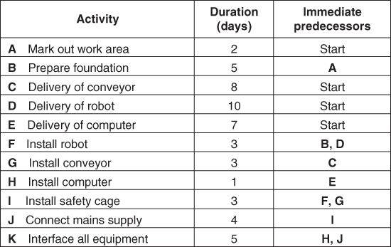
Figure 22.3 Example project list of activities and durations.
The simplest technique to use to represent this data is the basic Gantt chart. This is shown in Figure 22.4. The major project activities are listed down the left‐hand side of the chart and the days represented by columns; calendar dates would probably be used in a real world application. Completed activities are shown as broad bars, activities not yet started or incomplete are shown as thick lines. The thick vertical line joining the two pointers is the present time indicator, the situation at the end of day 9 is shown in the chart. The main advantage of the Gantt chart is immediately apparent, that is, it is easy to obtain a quick impression of the state of the individual project activities at the present time. It can be seen quickly that activities A, B, C and E have all been completed on schedule, that activity G has been completed ahead of schedule and that activities D and H are behind schedule. It also shows that the project activities are all expected to be completed by day 25.

Figure 22.4 Project Gantt chart.
Although the Gantt chart is quick and easy to read regarding the progress of the project, it does have some disadvantages for use as a planning aid and for obtaining more detailed progress information. For example, it does not make it obvious that although activity H is behind schedule by two days it will not interfere with the overall completion time of the project, whereas the two day delay on element D will probably also delay the project completion by two days. As well as not giving a clear indication of the interdependence of the various activities, it also does not allow the planner to see what activities must be completed on schedule to ensure that the project is completed as planned. Neither does it allow the planner to see how much an activity may be delayed without influencing the start of other activities; this difference between the earliest and latest activity start time is termed ‘float’. A knowledge of activity interdependence and float is essential to the planner, as it can allow scarce resources to he applied where and when they will be most effective. This is particularly important where a large number of items and work elements are involved: in a real project these may number thousands. Network planning techniques have been developed to provide this necessary information, the most popular of them being CPA and the Program Evaluation Review Technique (PERT) both developed in the USA in the 1950s. We will briefly examine the Critical Path Analysis (CPA) method here.
The first four steps in the CPA technique have already been carried out, that is, the project has been defined, the activities of which the project will be comprised have been listed, precedence relationships have been established and estimates of the activity durations have been made. The next stage is to construct a network of nodes and arrows. The convention we will use involves representing an activity by an arrow and representing an event, that is, the beginning or end of an activity, by a node. Thus the arrows represent a period of time whereas the nodes represent a point in time. Figure 22.5 shows the network for our project. As can be seen, it provides all the information we need regarding precedence relationships and start and end times for each activity; it is constructed as follows:
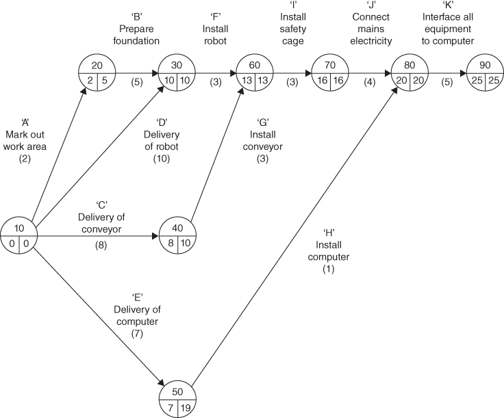
Figure 22.5 The critical path analysis for the project.
Using the previously compiled list of activities and precedence statements the start node is identified; in this case it may be assumed to be the point at which final approval is given for immediate commencement of the project. From this node arrows are drawn for each activity that can begin immediately the project starts. Each node is shown as a circle. The top half of the circle shows the node number; these are in multiples of 10 to allow the addition of extra nodes should this be found necessary. The bottom half of the node circle is split into two; the reason for this is explained later. For example, in Figure 14.6, node 10 is the start point for activities ‘A’, ‘C’, ‘D’ and ‘E’, and node 40 is the finish point for activity ‘C’. Node 40 is also the start of activity ‘G’ and node 60 its finish; the logic of the network is such that activity ‘G’ cannot start until activity ‘C’ is finished. If we now look at node 60 we see that two arrows enter this representing activities ‘F’ and ‘G’; this shows us that activity ‘I’ cannot commence until both activities ‘F’ and ‘G’ are completed. Using the arrows and nodes in this way, the network can be constructed. Further refinements are often necessary, such as the insertion of ‘dummy’ activities to allow precedence relationships to be represented that would otherwise be difficult to show.
The next stage is to carry out a forward pass through the network to determine the earliest event time for each node. For example, node 10 marking the start of the project is assumed to be day zero, although a calendar date would probably be inserted here in practice. Activity ‘A’ takes two days, thus the earliest time for node 20 is after two days; the number 2 is therefore entered in the bottom left of the node circle. Node 30, however, represents the completion of both activities ‘B’ and ‘D’. This means that it cannot exist until both of these activities have been completed. We must therefore insert into the bottom left space the maximum event time elapsed at that point. Since activity ‘B’ takes five days, a total of seven days will have elapsed by the time ‘B’ is completed.
However, since activity ‘D’ takes 10 days it is this value that must be inserted into the node as the earliest event time. This process is carried out throughout the network until the earliest completion date for the project can be entered into the final node. Examination of Figure 22.5 shows that this earliest completion date is 25 days after the project start.
Next a backward pass is carried out to determine the latest event time for each node. This will show the planner the latest each activity can be completed yet still maintain the earliest completion date. It follows logically that this process should also highlight those activities that must be completed according to schedule. The backward pass is carried out in a similar manner to the forward one, except that this time the activity durations are progressively subtracted and the results entered into the bottom right‐hand sector of the node circle. The difference in value between the right‐ and left‐hand numbers represents the ‘float’ time at that point. For example, the computer may arrive any time between day 7 and day 19 without affecting the earliest completion date of the project – that is, activity ‘E’, the delivery of the computer, has a float of 12 days.
The backward pass will also show up those activities with zero float. These activities meet at nodes where the earliest and latest node event times are identical. The network path created by these activities is termed the Critical Path and all activities on this path must be completed on time if the project is to finish on schedule. The critical path for our project passes from node 10, through nodes 30, 60, 70 and 80, to node 90.
Using this information the planner will now create a schedule for the project. Usually, each event will be scheduled to start at the earliest possible time to provide maximum float; this may be modified if two parallel activities demand the same resources, for example, specialised labour. To monitor the progress of the project, the planner may also construct a work schedule chart. This is a variation on the Gantt chart and is illustrated in Figure 22.6. The situation at the end of day 12 is shown and all work to date has been completed to plan. However, since the critical path is shown along the top of the chart, the planner or project manager will immediately recognise a serious delay should one occur on these activities. The float available on the other activities is also shown as broken lines; therefore, as long as the block showing the activity duration does not move beyond the broken lines the project may still be completed according to schedule.
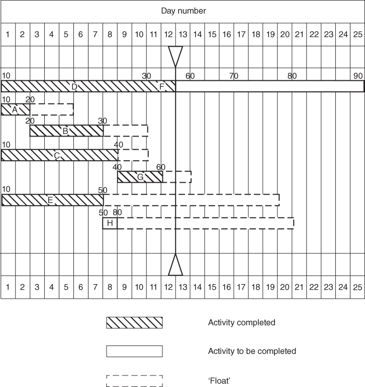
Figure 22.6 The project work schedule chart.
22.5 Process Planning
In order to make a component by any production process it is necessary first to create a plan of how the component will be made. The selection of which process to use has already been covered in Chapter 17; here, we consider the means used to plan the detail of manufacture. Some processes require a smaller number of operations than others to make a component. For example, the process planning for making a component by injection moulding is simple, for example, inject the plastic into the mould, remove component from mould when cool, trim excess material and place component on pallet. However, the sequence of operations is often more complex and this is particularly apparent when producing components by machining. As well as planning the manufacture of individual components, the assembly of these components into a finished product must also be planned; this requires the use of slightly different planning techniques. Process planning also allows labour and capacity requirements to be studied and an accurate estimate to be made of the time taken to produce the component or complete product. These aspects are considered more fully in Chapter 24.
Various types of charts may be constructed as aids to process planning. ‘Assembly charts’ are used to show the sequence of assembly and relationships between manufactured and bought out components and sub‐assemblies. They are particularly useful when complex products comprising many components and sub‐assemblies are being produced.
More detailed descriptions are then produced by creating ‘operations charts’ that now show the individual manufacturing and inspection operations, processes and equipment required. Further refinement is obtained by using ‘flow process charts’ that include additional information on transportation and storage. An indication of the type of charts being discussed can be seen in Figure 24.4, where a process chart for a product is shown.
Production of components by the machining processes often provides the most challenging aspects of this type of planning; despite the relative inefficiency of the process it remains a common problem for the planner. Computer aided process planning, CAPP, is used in industry, but due to the large number of variables, complexity and general need for experiential decisions, some amount of human input is usually required. The type of machines and the skill of the labour involved have a great influence on the length and detail of the process plan. For example, the use of numerically controlled machine tools reduces the amount of handling of the workpiece and the number of times the tooling has to be changed or adjusted, inspection operations are reduced and, apart from relatively simple work, holding devices jigs and fixtures are not required. Skilled craftsmen, such as toolmakers, do not require such detailed planning instruction as unskilled workers. In fact, an experienced toolmaker will be able to make a component or product by simply working from the engineering drawings, whereas an unskilled production worker will require detailed instructions on what material and machines to use, and the sequence of operations to be followed. Naturally, if a computer controlled process is being used such as a numerically controlled machine, the required information is held in the machine program and the machine operator simply has to load the material and unload the finished component.
To conclude this section a simplified example of an ‘operation layout sheet’ is shown in Figure 22.7 for a clevis rod (the clevis assembly is shown in Figure 24.4). For more complex machined components there are general guidelines that should be followed when preparing the operation layout. For example, at least one datum surface should be established as soon as machining commences. This datum will be used as a reference surface for all subsequent operations. To maximise accuracy, as many surfaces as possible should be created at the same setting; that is, without unclamping the workpiece in the machine. The use of surfaces as secondary references other than the original datum should be avoided as long as possible. Precision operations or those producing a smooth finished surface should be created last in order to reduce the possibility of damage. Finally, inspection operations should be included at appropriate intervals to minimise scrap and rework.
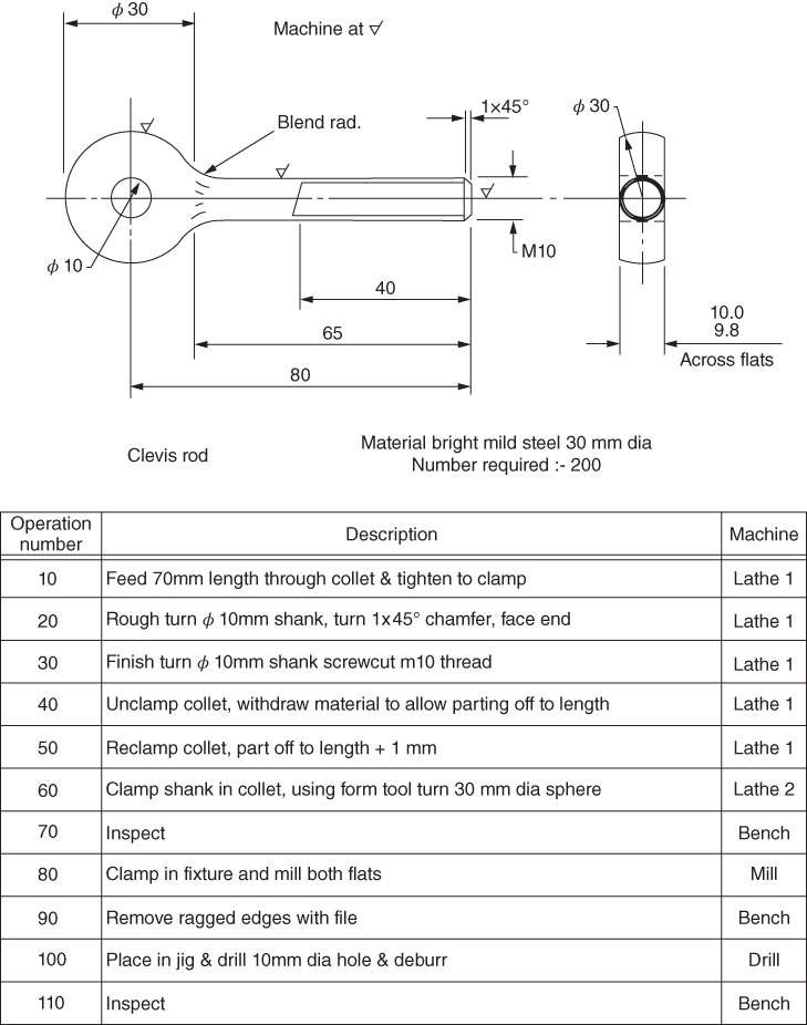
Figure 22.7 An operation layout sheet for a clevis rod.
Review Questions
- 1 List 10 criteria a company might use to decide where to locate a new factory and discuss the implications of each.
- 2 Describe how a company might use a decision matrix to assist with its location decision.
- 3 Briefly describe six types of plant layout.
- 4 What benefits should a company gain by careful attention to its factory layout?
- 5 Compare the advantages and disadvantages of functional and product layouts.
- 6 What do you understand by the term. ‘workpiece classification/coding’ and what benefits might a company gain by carefully applying its principles?
- 7 Explain the term ‘Group Technology’ (GT) and the type of plant layout associated with it.
- 8 Apart from material flow, list and discuss some of the things that should be given careful consideration when making decisions on plant layout.
- 9 What is a ‘Gantt Chart’, how is it used and what are its limitations for project planning?
- 10 Identify and list the steps to be followed in carrying out a CPA of a project.
- 11 What is meant by the terms ‘activity’, ‘node’, ‘activity interdependence’, ‘float’ and ‘critical path’ in CPA?
- 12 Consider the following project information (St = ‘start’)
Activity A B C D E F G H I J K L Duration 4 6 4 2 8 6 12 4 4 12 4 4 Predecessor St A St St B, C E D G D I J F, H, K Construct the network for this, identify the float for each activity and show the critical path.
- 13 Describe the function of the ‘work schedule chart’ and explain how it is an improvement on the basic Gantt chart.
- 14 What is the purpose of ‘process planning’ and how might the type of machinery and labour in use in a factory influence the process planning operation?
- 15 What is the purpose of an ‘operation layout sheet’ and what sort of guidelines should be followed by the planner as he or she constructs it?