
3.2 Proofs for Section 2.2.3 “Second-Order Spectral Characterization”
3.2.1 The μ Functional
In this section, the μ functional is introduced. It is defined as the functional whose value is the infinite-time average of the test function. The μ functional is formally characterized as the limit of approximating functions similar to the characterization of the Dirac delta as the limit of delta-approximating functions (Zemanian 1987, Section 1.3).
Let μ be the functional that associates to a test function ϕ its infinite-time average value. That is,
(3.16) ![]()
provided that the limit exists (and, hence, is independent of t).
In the following, the μ functional is heuristically characterized through formal manipulations. Let it be
(3.17) ![]()
where rect(t) = 1 for |t| ≤ 1/2 and rect(t) = 0 otherwise. For any finite T one has
(3.18) ![]()
Thus, in the limit as T→ ∞, we (rigorously) have
(3.19) 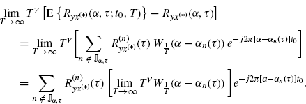
and we can formally write
with rhs independent of t, where μ(t) is formally defined as (see also (Silverman 1957))
In the sense of the ordinary functions, the limit in the rhs of (3.21) is the identically zero function. However, observing that for any finite T it results
(3.22) ![]()
then, in the limit as T→ ∞, we (rigorously) have
(3.23) ![]()
and we can formally write
That is, μ(t) can be interpreted as the limit of a very tiny and large rectangular window with unit area. This limit, of course, is the identically zero function in spaces of ordinary functions. However μ(t) can be formally managed as an ordinary function satisfying (3.20) and (3.24) similar to the formal manipulations of the Dirac delta.
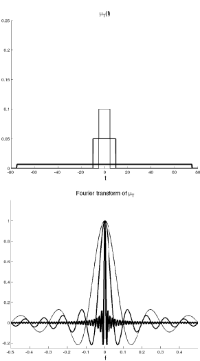
The Fourier transform of μ(t) can be formally derived by the following “limit passage.” Accounting for the Fourier transform pair
(3.25) ![]()
we can formally write (Figure 3.1)
where δf is the Kronecker delta, that is, δf = 1 for f = 0 and δf = 0 for f ≠ 0. Thus, μ(t) cannot be expressed as ordinary inverse Fourier transform (Lebesgue integral) since the Kronecker delta δf is zero a.e.
Figure 3.1 (Top) Function μT(t) and (bottom) its Fourier transform for increasing values of T (form thin line to thick line)
The following properties of the μ functional can be formally proved.
(3.28) 
3.2.2 Proof of Theorem 2.2.22 Loève Bifrequency Spectrum of GACS Processes
From Theorem 2.2.7 (t + τ = t1 and t = t2 in (2.18)) we have
(3.31) 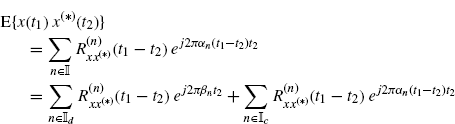
Thus, we formally have
(3.32) 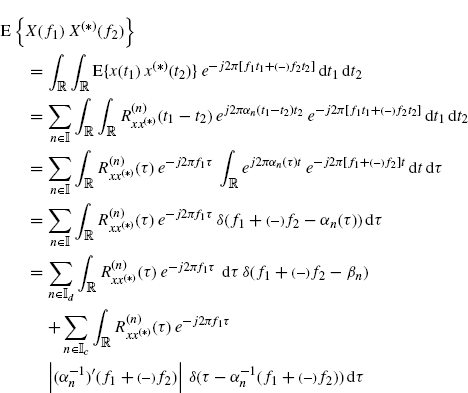
where, in the third equality, the variable change t1 = t + τ and t2 = t is made and in the fourth equality (2.71) and (2.72) are used. Then, (2.70) immediately follows.