
2.4 Estimation of the Cyclic Cross-Correlation Function
Let x(t) and y(t) be jointly GACS stochastic processes with cross-correlation function (2.31a)–(2.31c). In Sections 2.4–2.8 and 3.4–3.13, when it does not create ambiguity, for notation simplification we will put
![]()
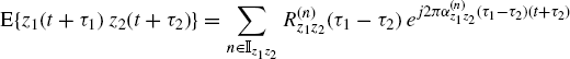
From (2.31b), it follows that the knowledge of the cyclic cross-correlation function ![]() , as a function of the two variables α and τ, completely characterizes the second-order cross-moments of jointly GACS processes. For each τ,
, as a function of the two variables α and τ, completely characterizes the second-order cross-moments of jointly GACS processes. For each τ, ![]() is nonzero only for those values of α such that
is nonzero only for those values of α such that ![]() for some
for some ![]() (see (2.39)). Moreover, for (α, τ) such that
(see (2.39)). Moreover, for (α, τ) such that ![]() for some
for some ![]() , the magnitude and phase of
, the magnitude and phase of ![]() are the amplitude and phase of the finite-strength additive complex sinewave component at frequency α contained in the cross-moment
are the amplitude and phase of the finite-strength additive complex sinewave component at frequency α contained in the cross-moment ![]() (see (2.31c) and (2.39)). Therefore, the problem of estimating second-order cross-moments of jointly GACS processes reduces to estimating the cyclic cross-correlation function as a function of the two variables (α, τ).
(see (2.31c) and (2.39)). Therefore, the problem of estimating second-order cross-moments of jointly GACS processes reduces to estimating the cyclic cross-correlation function as a function of the two variables (α, τ).
2.4.1 The Cyclic Cross-Correlogram
In this section, for jointly GACS processes, the cyclic cross-correlogram, the cyclic correlogram, and the conjugate cyclic correlogram are proposed as estimators of the cyclic cross-correlation function (2.33), the cyclic autocorrelation function (2.12), and the conjugate cyclic autocorrelation function (2.26), respectively. Moreover, their expected value and covariance are determined for finite data-record length (Napolitano 2007a).
Definition 2.4.1 Let ![]() and
and ![]() be continuous-time stochastic processes. Their cyclic cross-correlogram at cycle frequency
be continuous-time stochastic processes. Their cyclic cross-correlogram at cycle frequency ![]() is defined as
is defined as
where ![]() is a unit-area data-tapering window nonzero in (− T/2, T/2).
is a unit-area data-tapering window nonzero in (− T/2, T/2).
Note that since ![]() has finite width, the integral in (2.118) is extended to
has finite width, the integral in (2.118) is extended to ![]()
![]() . Consequently, the cycle-frequency resolution is of the order of 1/T.
. Consequently, the cycle-frequency resolution is of the order of 1/T.
By specializing (2.118) for ![]() and (*) present, one obtains the cyclic correlogram. For
and (*) present, one obtains the cyclic correlogram. For ![]() and (*) absent, one obtains the conjugate cyclic correlogram.
and (*) absent, one obtains the conjugate cyclic correlogram.
Assumption 2.4.2 Uniformly Almost-Periodic Statistics.
Assumption 2.4.3 Fourier Series Regularity.

A necessary condition such that (2.121) holds is that there exists a positive number M such that
(2.123) 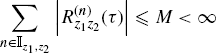
uniformly with respect to τ.
Assumption 2.4.4 Fourth-Order Moment Boundedness. The stochastic processes ![]() and
and ![]() have uniformly bounded fourth-order absolute moments. That is, for any
have uniformly bounded fourth-order absolute moments. That is, for any ![]() there exists a positive number
there exists a positive number ![]() such that
such that
(2.124) ![]()
Assumptions 2.4.2–2.4.4 regard time behavior and regularity of second-and fourth-order (joint) statistical functions of x(t) and y(t). Specifically, under such assumptions the second-order (cross-) moments of x(t) and y(t) and their fourth-order joint cumulants are limits of uniformly convergent sequences of trigonometricR polynomials in t. Moreover, for each Fourier series in (2.119) and (2.120), the nth coefficient has amplitude approaching zero, as n → ∞, sufficiently fast to assure that the infinite sums in (2.121) and (2.122) are convergent. A sufficient condition such that Assumption 2.4.4 holds is that the fourth-order moment functions of x(t) and y(t) are almost-periodic in t in the sense of Besicovitch.
Assumption 2.4.5 Data-Tapering Window Regularity. ![]() is a T -duration data-tapering window that can be expressed as
is a T -duration data-tapering window that can be expressed as
with ![]() , continuous almost everywhere (a.e.),
, continuous almost everywhere (a.e.),
[Note that (2.127) is used only to prove (3.66)].
Let ![]() be the Fourier transform of
be the Fourier transform of ![]() . In Section 3.5 (Lemma 3.5.1), it is shown that
. In Section 3.5 (Lemma 3.5.1), it is shown that ![]() . Let us assume that there exists
. Let us assume that there exists ![]() such that
such that ![]() as
as ![]() .
.
In the proofs of the asymptotic properties of the discrete-time cyclic cross-correlogram (Section 2.6) we also need the assumptions that a(t) is bounded and continuous in (− 1/2, 1/2) except, possibly, at ![]() is Riemann integrable, and is differentiable almost everywhere (a.e.) with bounded first-order derivative
is Riemann integrable, and is differentiable almost everywhere (a.e.) with bounded first-order derivative ![]() (see Lemmas 3.10.1 and 3.10.2).
(see Lemmas 3.10.1 and 3.10.2).
Assumption 2.4.5 is easily verified by taking a(t) with finite support [− 1/2, 1/2] and bounded (e.g., a(t) = rect(t)). If a(t) is continuous at t = 0, then from (2.127) it follows a(0) = 1.
The data-tapering window ![]() , strictly speaking, is a lag-product-tapering-window depending on the lag parameter τ. Its link with the signal-tapering window is discussed in Section 3.5, Fact 3.5.3.
, strictly speaking, is a lag-product-tapering-window depending on the lag parameter τ. Its link with the signal-tapering window is discussed in Section 3.5, Fact 3.5.3.
By taking the expected value of the cyclic cross-correlogram (2.118) and using (2.31c), the following result is obtained, where the assumptions allow to interchange the order of expectation, integral, and sum operations.
Theorem 2.4.6 Expected Value of the Cyclic Cross-Correlogram (Napolitano 2007a, Theorem 3.1). Let y(t) and x(t) be wide-sense jointly GACS stochastic processes with cross-correlation function (2.31c). Under Assumptions 2.4.5a (uniformly almost-periodic statistics), 2.4.3a (Fourier series regularity), and 2.4.5 (data-tapering window regularity), the expected value of the cyclic cross-correlogram ![]() is given by
is given by
where ![]() is the Fourier transform of
is the Fourier transform of ![]() .
.
Proof: See Section 3.4.
The function ![]() has duration T and, hence,
has duration T and, hence, ![]() has a bandwidth of the order of 1/T. Consequently, from (2.128), it follows that in the (α, τ)-plane the expected value of the cyclic cross-correlogram can be significantly different form zero within strips of width 1/T around the support curves
has a bandwidth of the order of 1/T. Consequently, from (2.128), it follows that in the (α, τ)-plane the expected value of the cyclic cross-correlogram can be significantly different form zero within strips of width 1/T around the support curves ![]() , of the cyclic cross-correlation function. Moreover, the expected value along a given lag-dependent cycle-frequency curve
, of the cyclic cross-correlation function. Moreover, the expected value along a given lag-dependent cycle-frequency curve ![]() is influenced not only by
is influenced not only by ![]() , but also by the values of the generalized cyclic cross-correlation functions
, but also by the values of the generalized cyclic cross-correlation functions ![]() relative to all the other lag-dependent cycle-frequency curves
relative to all the other lag-dependent cycle-frequency curves ![]() , the influence being stronger from curves
, the influence being stronger from curves ![]() closer to
closer to ![]() and with larger
and with larger ![]() . The effect becomes negligible as T → ∞. Such a phenomenon, in the case of cyclic statistic estimates of ACS processes is referred to as cyclic leakage (Gardner 1987d).
. The effect becomes negligible as T → ∞. Such a phenomenon, in the case of cyclic statistic estimates of ACS processes is referred to as cyclic leakage (Gardner 1987d).
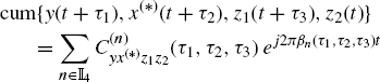
By expressing the covariance of the second-order lag-product ![]() in terms of second-order cross-moments and a fourth-order cumulant, the following result is obtained, where the assumptions allow to interchange the order of expectation, integral, and sum operations.
in terms of second-order cross-moments and a fourth-order cumulant, the following result is obtained, where the assumptions allow to interchange the order of expectation, integral, and sum operations.
Theorem 2.4.7 Covariance of the Cyclic Cross-Correlogram (Napolitano 2007a, Theorem 3.2). Let ![]() and
and ![]() be zero-mean wide-sense jointly GACS stochastic processes with cross-correlation function (2.31c). Under Assumptions 2.4.2 (uniformly almost-periodic statistics), 2.4.3 (Fourier series regularity), 2.4.4 (fourth-order moment boundedness), and 2.4.5 (data-tapering window regularity), the covariance of the cyclic cross-correlogram
be zero-mean wide-sense jointly GACS stochastic processes with cross-correlation function (2.31c). Under Assumptions 2.4.2 (uniformly almost-periodic statistics), 2.4.3 (Fourier series regularity), 2.4.4 (fourth-order moment boundedness), and 2.4.5 (data-tapering window regularity), the covariance of the cyclic cross-correlogram ![]() is given by
is given by
where
with
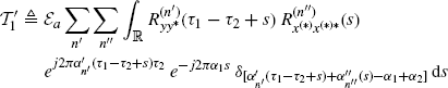
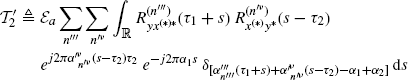
(2.134) ![]()
(2.135) ![]()
(2.136) ![]()
Proof: See Section 3.4.
For complex-valued processes, both covariance and conjugate covariance are needed for a complete second-order wide-sense characterization (Picinbono 1996), (Picinbono and Bondon 1997), (Schreier and Scharf 2003a,b). The expression of the conjugate covariance of the cyclic cross-correlogram can be obtained by reasoning as for Theorem 2.4.7 and is reported in Section 3.7.
Finally, note that in the special case of ACS processes, Theorems 2.4.6 and 2.4.7 reduce to well-known results of (Hurd 1989a, 1991), (Hurd and Le![]() kow 1992b), (Dehay and Hurd 1994), (Genossar et al. 1994), (Dandawaté and Giannakis 1995).
kow 1992b), (Dehay and Hurd 1994), (Genossar et al. 1994), (Dandawaté and Giannakis 1995).
2.4.2 Mean-Square Consistency of the Cyclic Cross-Correlogram
In this section, the cyclic cross-correlogram is shown to be a mean-square consistent estimator of the cyclic cross-correlation function (Napolitano 2007a).
Assumption 2.4.8 Mixing Conditions (I).
In the proofs of the asymptotic properties of the discrete-time cyclic cross-correlogram (Section 2.6) we also need the assumption that the functions ![]() and
and ![]()
![]() are Riemann integrable.
are Riemann integrable.
Assumptions 2.4.8a and 2.4.8b are referred to as mixing conditions and are generally satisfied if the involved stochastic processes have finite or practically finite memory, i.e., if z1(t) and z2(t + s) are asymptotically ![]() independent (Section 1.4.1), (Brillinger and Rosenblatt 1967). For example, under assumption (2.121), the function series
independent (Section 1.4.1), (Brillinger and Rosenblatt 1967). For example, under assumption (2.121), the function series ![]() is uniformly convergent due to the Weierstrass criterium (Smirnov 1964). In addition, in order to satisfy (2.137), the function
is uniformly convergent due to the Weierstrass criterium (Smirnov 1964). In addition, in order to satisfy (2.137), the function ![]() should be vanishing sufficiently fast as
should be vanishing sufficiently fast as ![]() in order to be summable. A sufficient condition is that there exists
in order to be summable. A sufficient condition is that there exists ![]() > 0 such that
> 0 such that ![]()
![]() , where
, where ![]() is the “big oh” Landau symbol.
is the “big oh” Landau symbol.
Assumption 2.4.8b is used to prove the asymptotic vanishing of the covariance of the cyclic cross-correlogram in Theorem 2.4.13. This condition, however, is not sufficient to obtain a bound for the covariance uniform with respect to α1, α2, τ1, τ2. Uniformity is obtained in Corollary 2.4.14 with the following further assumption.
Assumption 2.4.9 Mixing Conditions (II). For any choice of z1 in {y, y*} and z2 in {x, x*} there exist functions ϕ(n)(s) such that
(2.139) ![]()
with
(2.140) ![]()
![]()
Assumption 2.4.9 implies Assumption 2.4.8b with the left-hand side of (2.138) uniformly bounded with respect to τ1 and τ2.
Assumption 2.4.10 Lack of Support Curve Clusters (I). There is no cluster of support curves. That is, let
then for every α0 and τ0, for any ![]() no curve αn(τ) can be arbitrarily close to the value α0 for τ = τ0. Thus, for any α and τ it results in
no curve αn(τ) can be arbitrarily close to the value α0 for τ = τ0. Thus, for any α and τ it results in
![]()
The set ![]() contains the only element
contains the only element ![]() if
if ![]() is the only support curve such that
is the only support curve such that ![]() . The set
. The set ![]() contains more elements if (α0, τ0) is a point where more support curves intercept each other (see (2.20) and (2.21)). The set
contains more elements if (α0, τ0) is a point where more support curves intercept each other (see (2.20) and (2.21)). The set ![]() is empty if α0 ≠ αn(τ0)
is empty if α0 ≠ αn(τ0) ![]() .
.
Assumption 2.8 is used to establish the rate of convergence to zero of the bias and the asymptotic Normality of the cyclic cross-correlogram. In the special case of ACS signals, Assumption 2.8 means that there is no cycle frequency cluster point (see (Hurd 1991), (Dehay and Hurd 1994)).
By taking the limit of the expected value of the cyclic cross-correlogram (2.128) as the data-record length T approaches infinite, the following result is obtained, where the assumptions allow to interchange the order of limit and sum operations.
Theorem 2.4.11 Asymptotic Expected Value of the Cyclic Cross-Correlogram (Napolitano 2007a, Theorem 4.1). Let y(t) and x(t) be wide-sense jointly GACS stochastic processes with cross-correlation function (2.31c). Under Assumptions 2.4.2a (uniformly almost-periodic statistics), 2.4.3a (Fourier series regularity), and 2.4.5 (data-tapering window regularity), the asymptotic expected value of the cyclic cross-correlogram ![]() is given by
is given by
Proof: See Section 3.5. ![]()
Let A(f) be the Fourier transform of a(t) with rate of decay to zero |f|−γ for |f|→ ∞ as specified in Assumption 2.5. For the bias of the cyclic cross-correlogram
(2.144) ![]()
the following result holds.
Theorem 2.4.12 Rate of Convergence of the Bias of the Cyclic Cross-Correlogram (Napolitano 2007a, Theorem 4.2). Let y(t) and x(t) be wide-sense jointly GACS stochastic processes with cross-correlation function (2.31c). Under Assumptions 2.4.2a (uniformly almost-periodic statistics), 2.4.3a (Fourier series regularity), 2.4.5 (data-tapering window regularity), and 2.4.10 (lack of support curve clusters (I)), one obtains
Proof: See Section 3.5. ![]()
We are interested in finding the maximum of the values of γ such that (2.145) holds, provided that such a maximum exists. This can be achieved, for example, by observing that if a(t) is p times differentiable and the p-th order derivative a(p)(t) is summable, then ![]() , where
, where ![]() denotes the L1-norm. As further examples, a(t) = rect(t) ⇒ A(f) = sinc(f) ⇒ γ = 1; a(t) = (1 − |t|)rect(t/2) ⇒ A(f) = sinc2(f) ⇒ γ = 2. Furthermore, the result of Theorem 2.4.12 can be extended with minor changes to the case A(f) = O(g(f)) as |f|→ ∞, with g(f) strictly increasing function with no order of infinity (e.g., g(|f|) = |f| ln |f|).
denotes the L1-norm. As further examples, a(t) = rect(t) ⇒ A(f) = sinc(f) ⇒ γ = 1; a(t) = (1 − |t|)rect(t/2) ⇒ A(f) = sinc2(f) ⇒ γ = 2. Furthermore, the result of Theorem 2.4.12 can be extended with minor changes to the case A(f) = O(g(f)) as |f|→ ∞, with g(f) strictly increasing function with no order of infinity (e.g., g(|f|) = |f| ln |f|).
In Fact 3.5.3, the link between the signal-tapering window and the lag-product-tapering window is established. Consequences of this link on the rate of convergence of bias are discussed in Section 3.5.
Starting from Theorem 2.4.7, the following result is obtained, where the assumptions allow to interchange the order of limit and sum operations.
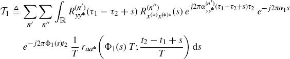
Theorem 2.4.13 Asymptotic Covariance of the Cyclic Cross-Correlogram (Napolitano 2007a, Theorem 4.3). Let y(t) and x(t) be zero-mean wide-sense jointly GACS stochastic processes with cross-correlation function (2.31c). Under Assumptions 2.4.2 (uniformly almost-periodic statistics), 2.4.3 (Fourier series regularity), 2.4.4 (fourth-order moment boundedness), 2.4.5 (data-tapering window regularity), and 2.4.8 (mixing conditions (I)), the asymptotic covariance of the cyclic cross-correlogram ![]() is given by
is given by
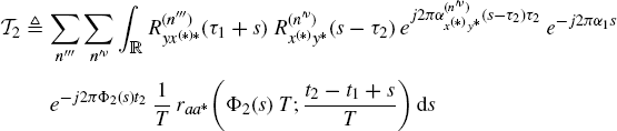
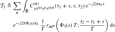
where
with![]() . In (2.147)–(2.149), for notation simplicity,
. In (2.147)–(2.149), for notation simplicity, ![]() ,
, ![]() ,
, ![]() , and
, and ![]() .
.
Proof: See Section 3.5. ![]()
Theorem 2.4.13 can also be proved by substituting the mixing condition in Assumption 2.6 a with the mixing condition in Assumption 3.5.4 as explained in Section 3.5.
In Theorem 2.4.13, the terms in (2.147), (2.148), and (2.149) can give nonzero contribution only if the argument of the Kronecker deltas is zero in a set of values of s with a positive Lebesgue measure. For example, if the signals x(t) and y(t) are singularly and jointly purely GACS (Section 2.2.2), then in (2.147) with α1 = α2 and τ1 = τ2, the terms with ![]() can give nonzero contribution.
can give nonzero contribution.
From Theorem 2.4.11 it follows that the cyclic cross-correlogram (2.118), as a function of ![]() , is an asymptotically unbiased estimator of the cyclic cross-correlation function (2.33). Moreover, from Theorem 2.4.13 it follows that its variance
, is an asymptotically unbiased estimator of the cyclic cross-correlation function (2.33). Moreover, from Theorem 2.4.13 it follows that its variance
(2.150) ![]()
is O(T−1) as T→ ∞. Therefore, since
(2.151) 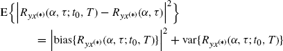
the cyclic cross-correlogram is a mean-square consistent estimator of the cyclic cross-correlation function.
The expression of the asymptotic conjugate covariance of the cyclic cross-correlogram is reported in Section 3.7.
By specializing Theorems 2.4.11 –2.4.13 for y = x and (*) present, we have that the cyclic correlogram is a mean-square consistent estimator of the cyclic autocorrelation function. For y = x and (*) absent, we have that the conjugate cyclic correlogram is a mean-square consistent estimator of the conjugate cyclic autocorrelation function.
For ACS processes, we obtain as a special case results of (Hurd 1989a, 1991), (Hurd and Le![]() kow 1992b), (Dehay and Hurd 1994), (Genossar et al. 1994), (Dandawatacute; and Giannakis 1995), (Schell 1995). In particular, in the asymptotic covariance (2.146), the terms
kow 1992b), (Dehay and Hurd 1994), (Genossar et al. 1994), (Dandawatacute; and Giannakis 1995), (Schell 1995). In particular, in the asymptotic covariance (2.146), the terms ![]() ,
, ![]() and
and ![]() defined in (2.147), (2.148), and (2.149) specialize into
defined in (2.147), (2.148), and (2.149) specialize into
(2.152) ![]()
(2.153) ![]()
(2.154) ![]()
where the sum over n′ is extended to all cycle frequencies ![]() of
of ![]() such that
such that ![]() is a cycle frequency of
is a cycle frequency of ![]() , the sum over n′′ ′ is extended to all cycle frequencies
, the sum over n′′ ′ is extended to all cycle frequencies ![]() of
of ![]() such that
such that ![]() is a cycle frequency of
is a cycle frequency of ![]() , and the last term is nonzero only if α1 − α2 is a (fourth-order) cycle frequency of
, and the last term is nonzero only if α1 − α2 is a (fourth-order) cycle frequency of ![]() .
.
The asymptotic bias (Theorem 2.4.12), in general, is not uniform with respect to α and τ. In fact, from (2.128) and the continuity of ![]() (Lemma 3.5.1a),
(Lemma 3.5.1a), ![]() is a continuous function of α for each fixed τ at least in the case of
is a continuous function of α for each fixed τ at least in the case of ![]() finite or for
finite or for ![]() approaching zero sufficiently fast as n→ ∞. In contrast, since for each fixed τ the set Aτ defined in (2.32a) is countable, the function
approaching zero sufficiently fast as n→ ∞. In contrast, since for each fixed τ the set Aτ defined in (2.32a) is countable, the function ![]() is discontinuous in α (see also (2.39)). Thus, we have the convergence of a family of continuous functions to a discontinuous function and, hence, the convergence cannot be uniform. In particular, the closer the point (α, τ) is to a support curve, the slower the convergence of the estimator bias. An analogous result was found in (Genossar et al. 1994) for discrete-time asymptotically-mean cyclostationary processes. Furthermore, the asymptotic variance (Theorem 2.4.13) is not uniform with respect to α1, α2, τ1, and τ2. However, a bound for the covariance, uniform with respect to cycle frequencies and lag shifts can be obtained starting from Theorem 2.4.10 with the aid of Assumptions 2.6 a and 2.7. It is the analogous for continuous-time GACS processes of a similar result proved in (Genossar et al. 1994) for discrete-time asymptotically-mean cyclostationary processes.
is discontinuous in α (see also (2.39)). Thus, we have the convergence of a family of continuous functions to a discontinuous function and, hence, the convergence cannot be uniform. In particular, the closer the point (α, τ) is to a support curve, the slower the convergence of the estimator bias. An analogous result was found in (Genossar et al. 1994) for discrete-time asymptotically-mean cyclostationary processes. Furthermore, the asymptotic variance (Theorem 2.4.13) is not uniform with respect to α1, α2, τ1, and τ2. However, a bound for the covariance, uniform with respect to cycle frequencies and lag shifts can be obtained starting from Theorem 2.4.10 with the aid of Assumptions 2.6 a and 2.7. It is the analogous for continuous-time GACS processes of a similar result proved in (Genossar et al. 1994) for discrete-time asymptotically-mean cyclostationary processes.
Corollary 2.4.14 (Napolitano 2007a, Corollary 4.1). Let y(t) and x(t) be zero-mean wide-sense jointly GACS stochastic processes with cross-correlation function (2.31c). Under Assumptions 2.2 (uniformly almost-periodic statistics), 2.3 (Fourier series regularity), 2.4 (fourth-order moment boundedness), 2.5 (data-tapering window regularity), 2.6 (mixing conditions (I)), and 2.7 (mixing conditions (II)), there exists K such that
(2.155) ![]()
uniformly with respect to α1, α2, τ1, and τ2.
Proof: See Section 3.5. ![]()
2.4.3 Asymptotic Normality of the Cyclic Cross-Correlogram
In this section, the asymptotic complex Normality (Picinbono 1996), (van den Bos 1995) of the cyclic cross-correlogram is proved (Napolitano 2007a).
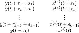
Let
(2.156) ![]()
be second-order lag-product waveforms, with optional complex conjugations [*]i, i = 1, ..., k, having kth-order cumulant
(2.157) ![]()
where the cumulant of complex processes is defined according to (Spooner and Gardner 1994, App. A) (see also Section 1.4.2).
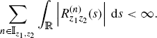
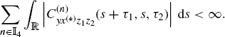
Assumption 2.4.15 Mixing Conditions (III). For every integer k ≥ 2, ![]() , i = 1, ..., k and every conjugation configuration [*]1, ..., [*]k, there exists a positive summable function ϕ(s1, ..., sk−1) (depending on τi, i = 1, ..., k and the conjugation configuration) such that
, i = 1, ..., k and every conjugation configuration [*]1, ..., [*]k, there exists a positive summable function ϕ(s1, ..., sk−1) (depending on τi, i = 1, ..., k and the conjugation configuration) such that
(2.158) ![]()
uniformly with respect to t. ![]()
The cumulant of the lag products zi(t) can be expressed in terms of cumulants of y(t + τj) and x(t). For this purpose, let us consider the k × 2 table
and a partition of its elements into disjoint sets {ν1, ..., νp}, that is, νi ∩ νj = ∅ for i ≠ j and ![]() the whole table. Then, let us denote each element of the table (2.159) by its row and column indices (
the whole table. Then, let us denote each element of the table (2.159) by its row and column indices (![]() , m). We say that the two sets
, m). We say that the two sets ![]() and
and ![]() hook if there exist
hook if there exist ![]() and
and ![]() such that
such that ![]() 1 =
1 = ![]() 2, that is, the two sets contain (al least) two elements with the same row index. We say that the sets
2, that is, the two sets contain (al least) two elements with the same row index. We say that the sets ![]() and
and ![]() communicate if there exists a sequence of sets
communicate if there exists a sequence of sets ![]() such that
such that ![]() and
and ![]() hook for each h. A partition is said to be indecomposable if all its sets communicate (Leonov and Shiryaev 1959), (Brillinger 1965), (Brillinger and Rosenblatt 1967). It can be seen that if r1, ..., rk denote the rows of the table (2.159), then the partition {ν1, ..., νp} is indecomposable if and only if there exist no sets
hook for each h. A partition is said to be indecomposable if all its sets communicate (Leonov and Shiryaev 1959), (Brillinger 1965), (Brillinger and Rosenblatt 1967). It can be seen that if r1, ..., rk denote the rows of the table (2.159), then the partition {ν1, ..., νp} is indecomposable if and only if there exist no sets ![]() , (n < p), and rows
, (n < p), and rows ![]() , (h < k), such that
, (h < k), such that ![]() ; that is, if and only if we cannot build a rectangle of size h × 2, with h < k, using some of the sets of the partition.
; that is, if and only if we cannot build a rectangle of size h × 2, with h < k, using some of the sets of the partition.
The cumulant ![]() can be expressed as (Leonov and Shiryaev 1959), (Brillinger 1965), (Brillinger and Rosenblatt 1967)
can be expressed as (Leonov and Shiryaev 1959), (Brillinger 1965), (Brillinger and Rosenblatt 1967)
where νi (i = 1, ..., p) are subsets of elements of the k × 2 table (2.159), ![]() is the cumulant of the elements in νi, and the (finite) sum in (2.160) is extended over all indecomposable partitions of table (2.159), including the partition with only one element (see (3.45) for the case k = 2 and zero-mean processes). Therefore, Assumption 2.9 is satisfied provided that the cumulants up to order 2k of the elements taken from table in (2.159) are summable with respect to the variables s1, ..., sk−1 and a bound uniform with respect to t exists. That is
is the cumulant of the elements in νi, and the (finite) sum in (2.160) is extended over all indecomposable partitions of table (2.159), including the partition with only one element (see (3.45) for the case k = 2 and zero-mean processes). Therefore, Assumption 2.9 is satisfied provided that the cumulants up to order 2k of the elements taken from table in (2.159) are summable with respect to the variables s1, ..., sk−1 and a bound uniform with respect to t exists. That is
Assumption 2.4.15 is referred to as a mixing condition and is fulfilled if the processes x(t) and y(t) have finite-memory or a memory decaying sufficiently fast. It generalizes to the nonstationary case, assumption made in (Brillinger 1965, eq. (5.5)) in the stationary case. Examples of processes satisfying Assumption 2.4.15 are communications signals with independent and identically distributed (i.i.d.) symbols or block coded symbols, processes with exponentially decaying joint probability density function, and finite-memory (time-variant) transformations of such processes.
For a single process x(t) (y ≡ x), according to the results of Section 1.4.1, the asymptotic statistical independence implies that, for every ![]() ,
,
(2.162) ![]()
where ![]() . Thus, the summability condition (2.161) is satisfied provided that
. Thus, the summability condition (2.161) is satisfied provided that
(2.163) ![]()
for some ![]() > 0, uniformly with respect to t, for every
> 0, uniformly with respect to t, for every ![]() ≤ 2k.
≤ 2k.
Assumption 2.4.15 turns out to be verified if the stochastic processes zi(t), i = 1, ..., k are jointly kth-order GACS (Section 2.2.4), (Izzo and Napolitano 1998a), that is
(uniformly almost-periodic in t in the sense of Besicovitch (Besicovitch 1932)) and, moreover,
Assumption 2.4.16 Cross-Moment Boundedness. For every ![]() and every {
and every { ![]() 1, ...,
1, ..., ![]() n} ⊆ {1, ..., k}, there exists a positive number
n} ⊆ {1, ..., k}, there exists a positive number ![]() such that
such that
(2.166) ![]()
![]()
Assumption 2.4.16 means that the processes y(t) and x(t) have uniformly bounded 2kth-order cross-moments for every k.
The proof of the zero-mean joint complex asymptotic Normality of the random variables
is given in Theorem 2.4.14 showing that asymptotically (T → ∞)
with superscript [*]h denoting optional complex conjugation. In fact, in Section 1.4.2 it is shown that these are necessary and sufficient conditions for the joint asymptotic Normality of complex random variables, where cumulants of complex random variables are defined according to (Spooner and Gardner 1994, App. A) (see also (1.209) and Section 1.4.2 for a discussion on the usefulness of this definition). Condition 1 follows from Theorem 2.4.12 on the rate of decay to zero of the bias of the cyclic cross-correlogram. Condition 2a is a consequence of Theorem 2.4.13 on the asymptotic covariance of the cyclic cross-correlogram. Condition 2b follows form Theorem 3.7.2. Finally, Condition 3 follows from Lemma 2.4.2 on the rate of decay to zero of the joint cumulant of cyclic cross-correlograms.
The main assumptions used to prove these theorems and lemmas are regularity of the (generalized) Fourier series of the almost-periodic second-and fourth-order cumulants of the processes (Assumptions 2.4.2 –2.4.3), short-range statistical dependence of the processes expressed in terms of summability of joint cumulants (Assumptions 2.4.8 and 2.4.15), lack of clusters of support curves (Assumption 2.4.10), and regularity of the data-tapering window (Assumption 2.4.5). In addition, Assumptions 2.4.4 and 2..4.16 on boundedness of moments are used for technicalities (application of the Fubini and Tonelli theorem).
Lemma 2.4.17 (Napolitano 2007a, Lemma 5.1). Under Assumptions 2.4.5 (data-tapering window regularity), 2.4.15 (mixing conditions (III)), and 2.4.16 (cross-moment boundedness), for any k ≥ 2 and ![]() > 0 one obtains
> 0 one obtains
Proof: See Section 3.6. ![]()
Theorem 2.4.18 Asymptotic Joint Normality of the Cyclic Cross-Correlograms (Napolitano 2007a, Theorem 5.1). Let x(t) and y(t) be zero mean. Under Assumptions 2.4.2 (uniformly almost-periodic statistics), 2.4.3 (Fourier series regularity), 2.4.4 (fourth-order moment boundedness), 2.4.5 (data-tapering window regularity), 2.4.8 (mixing conditions (I)), 2.4.10 (lack of support curve clusters (I)), 2.4.15 (mixing conditions (III)), 2.5.16 (cross-moment boundedness), and if ![]() in Theorem 2.4.12, one obtains that, for every fixed αi, τi, ti, i = 1, ..., k, the random variables
in Theorem 2.4.12, one obtains that, for every fixed αi, τi, ti, i = 1, ..., k, the random variables ![]() defined in (2.167)
defined in (2.167)
are asymptotically (T→ ∞) zero-mean jointly complex Normal with asymptotic covariance matrix Σ with entries
(2.169) ![]()
given by (2.146) and asymptotic conjugate covariance matrix Σ(c) with entries
(2.170) ![]()
given by (3.137).
Proof: See Section 3.6. ![]()
Corollary 2.4.19 Under the Assumptions for Theorem 2.4.18, one obtains that, for every fixed α, τ, t0, the random variable ![]() is asymptotically zero-mean complex Normal:
is asymptotically zero-mean complex Normal:
(2.171) ![]()
![]()
By specializing Theorem 2.4.18 and Corollary 2.4.19 for y = x and (*) present, we find that the cyclic correlogram is an asymptotically Normal estimator of the cyclic autocorrelation function. For y = x and (*) absent, we find that the conjugate cyclic correlogram is an asymptotically Normal estimator of the conjugate cyclic autocorrelation function. For ACS processes, we obtain as a special case the results of (Hurd and Le![]() kow 1992b), (Dehay and Hurd 1994), (Dandawatacute; and Giannakis 1995).
kow 1992b), (Dehay and Hurd 1994), (Dandawatacute; and Giannakis 1995).
As a final remark, note that here it was preferred to describe the finite or practically finite memory of the involved processes by assuming summability of (joint) cumulants of the processes. These assumptions turn out to be more easily verifiable than ϕ-mixing assumptions (Billingsley 1968, p. 166), (Rosenblatt 1974, pp. 213–214), (Hurd and Le![]() kow 1992a,b) which are expressed in terms of a function ϕ(s) which describes or controls the dependence between events separated by s time unites. In contrast, summability of cumulants can be derived from properties of the stochastic processes for which cumulants can be calculated (see e.g., (Gardner and Spooner 1994), (Spooner and Gardner 1994), (Napolitano 1995)). A discussion of the finite or practically finite memory of processes by using cumulants is given in Section 1.4.1 and (Brillinger 1965).
kow 1992a,b) which are expressed in terms of a function ϕ(s) which describes or controls the dependence between events separated by s time unites. In contrast, summability of cumulants can be derived from properties of the stochastic processes for which cumulants can be calculated (see e.g., (Gardner and Spooner 1994), (Spooner and Gardner 1994), (Napolitano 1995)). A discussion of the finite or practically finite memory of processes by using cumulants is given in Section 1.4.1 and (Brillinger 1965).