2.7 Numerical Results

In this section, simulation experiments are carried out, aimed at corroborating the theoretical results of the previous sections.

2.7.1 Aliasing in Cycle-Frequency Domain

In the simulation experiments, a GACS signal is obtained as the output of the Doppler channel existing between a transmitter and a receiver with constant relative radial acceleration, when the input signal is a cyclostationary PAM signal (Section 2.2.6.1). In this case, an analytical condition on the sampling frequency can be deduced, which limits aliasing. Starting from (2.179a) specialized for x ≡ y and ACS signals, it follows that aliasing in the cycle-frequency domain can be avoided, provided that f_s ≥ 4B, where B is the monolateral bandwidth of x(t) (Theorem 1.3.7), (Izzo and Napolitano 1996). Since 2B is the maximum allowable cycle frequency for an ACS signal with bandwidth B, condition f_s ≥ 4B prevents replicas in (2.179a) with p ≠ 0 from contributing to the discrete-time cyclic autocorrelation function in the “principal domain” . If x(t) is not strictly bandlimited, with approximate monolateral bandwidth B, then 2B is the maximum cycle frequency at which x(t) exhibits a significant degree of cyclostationarity. For the chirp-modulated signal y(t) in (2.99) with x(t) ACS, the effect of the chirp modulation is to rotate by an angle θ, where tan θ = γ, the support lines of the cyclic autocorrelation function of x(t) (see (2.104) and Figures 2.2 (bottom) and 2.3 (bottom)). Consequently, denoted by τ_corr the maximum value of |τ| such that (and, hence, ) is significantly different from zero, we have that the maximum cycle frequency exhibited by the GACS signal y(t) is 2B + τ_corr sin θ. Thus, the condition

(2.239)

is sufficient to prevent aliasing in the discrete-time cyclic autocorrelation function of the samples of y(t).

2.7.2 Simulation Setup

In the experiments, unless otherwise specified, the input signal is a PAM signal with a raised cosine pulse with excess bandwidth η = 0.85, a stationary white binary modulating sequence, and symbol period T_p = 10T_s, where T_s is the sampling period. Such a signal passes through a Doppler channel which produces a delay d₀ = 20T_s, a frequency shift ν = 0.02/T_s, and a chirp rate . The resulting output GACS signal is the chirp-modulated signal (2.99). Since the PAM signal has a white modulating sequence and the raised cosine pulse decay sufficiently fast as |t|→ ∞, its cyclic autocorrelation functions are summable. Moreover, since this PAM signal is strictly bandlimited, then the number of cycle frequencies is finite and Assumptions 2.4.3a and 2.4.8a turn out to be verified. Furthermore, similar considerations hold for the fourth-order cumulants. For the adopted values, condition (2.239) turns out to be verified.

2.7.3 Cyclic Correlogram Analysis with Varying N

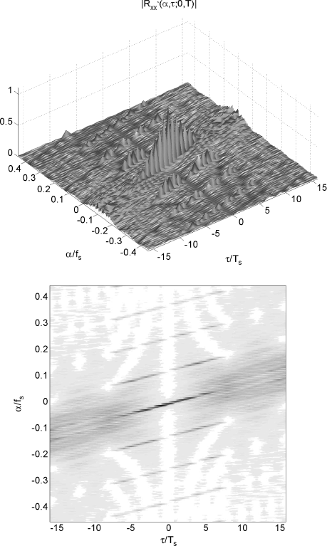
The sample mean and the sample standard deviation, computed by 400 Monte Carlo runs, of the cyclic correlogram of the samples of y(t) are evaluated for different data-record lengths T = NT_s and using a rectangular data-tapering window. For N = 2⁹, in Figure 2.5 (top) graph and (bottom) “checkerboard” plot of the magnitude of the sample mean of the cyclic correlogram, and in Figure 2.6 (top) graph and (bottom) “checkerboard” plot of the sample standard deviation of the cyclic correlogram are reported as functions of αT_s and τ/T_s. The same quantities are reported in Figures 2.7 and 2.8 for N = 2¹². The adopted data-record lengths N = 2⁹ and N = 2¹², correspond to about 52 and 411 symbols of the PAM signal. A discrete set of values of is considered by taking 400 cycle-frequency values in the cycle-frequency interval [− 1/4, 1/4).

Figure 2.5 Cyclic correlogram of the chirp-modulated signal (2.99) computed by a data-record length T = NT_s with N = 2⁹: (Top) graph and (bottom) “checkerboard” plot of the magnitude of the sample mean of the cyclic correlogram as a function of αT_s and τ/T_s.

Source: (Napolitano 2007a) © IEEE

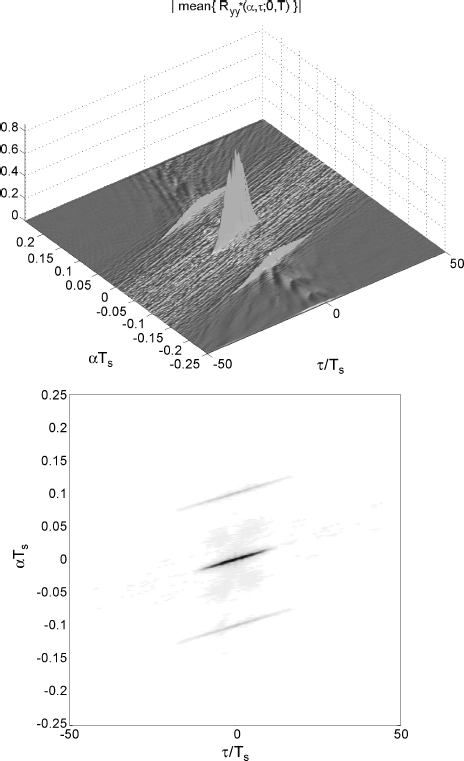
Figure 2.6 Cyclic correlogram of the chirp-modulated signal (2.99) computed by a data-record length T = NT_s with N = 2⁹: (Top) graph and (bottom) “checkerboard” plot of the sample standard deviation of the cyclic correlogram as a function of αT_s and τ/T_s.

Source: (Napolitano 2007a) © IEEE

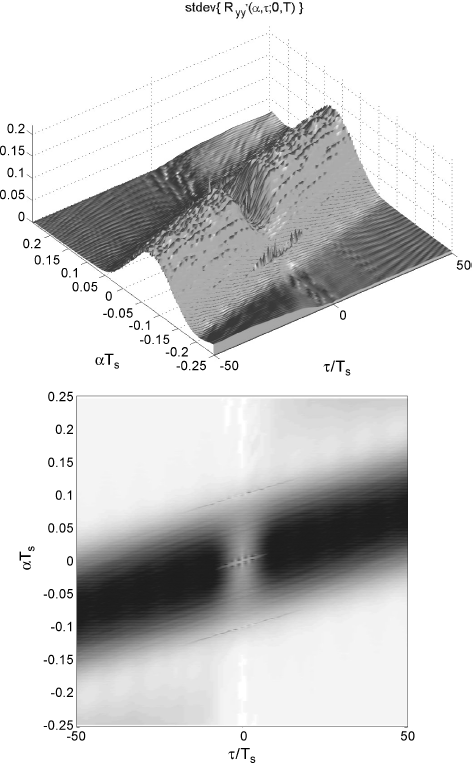
Figure 2.7 Cyclic correlogram of the chirp-modulated signal (2.99) computed by a data-record length T = NT_s with N = 2¹²: (Top) graph and (bottom) “checkerboard” plot of the magnitude of the sample mean of the cyclic correlogram as a function of αT_s and τ/T_s.

Source: (Napolitano 2007a) © IEEE

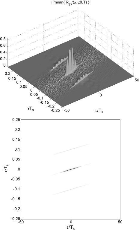
Figure 2.8 Cyclic correlogram of the chirp-modulated signal (2.99) computed by a data-record length T = NT_s with N = 2¹²: (Top) graph and (bottom) “checkerboard” plot of the sample standard deviation of the cyclic correlogram as a function of αT_s and τ/T_s.

Source: (Napolitano 2007a) © IEEE

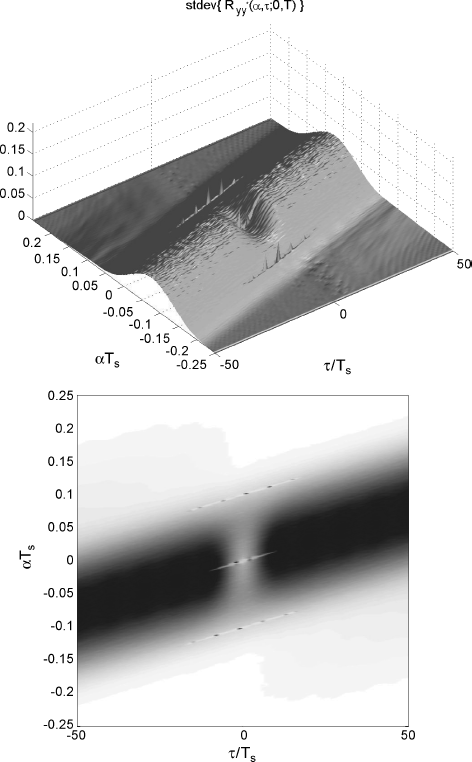
The numerical results corroborate the theoretical results of Section 2.4.2. In fact, as the data-record is increased from N = 2⁹ to N = 2¹², both bias and standard deviation decrease. Specifically, as regards the sample mean of the cyclic correlogram, the blurred region outside the support of the cyclic autocorrelation function exhibits reduced oscillations as N is increased (Figures 2.5 (top) and 2.7 (top)) and the sample mean approaches the true cyclic autocorrelation function (Figure 2.3 (top)). Moreover, the sample mean is significantly different from zero within thin strips around the true lag-dependent cycle frequencies and the strip width becomes narrower as the data-record is increased (see Figures 2.5 (bottom) and 2.7 (bottom) compared with Figure 2.3 (bottom)). Furthermore, the sample standard deviation decreases as N increases (Figures 2.6 (top) and 2.8 (top)).

2.7.4 Cyclic Correlogram Analysis with Varying N and T_s

In this section, results of experiments are reported to corroborate the results of Section 2.6.

The sample mean and the sample standard deviation, computed by 10⁴ Monte Carlo runs, of the discrete-time cyclic correlogram of the ACS discrete-time signal obtained by uniformly sampling the continuous-time GACS signal are evaluated for different numbers of data samples N and sampling periods T_s. The overall data-record length is T = NT_s. For a rectangular signal-tapering window, the continuous-time lag-product tapering window and its Fourier transform are given by (Fact 3.5.3)

(2.240)

(2.241)

respectively. Hence, according to the results of Section 2.6, the rate of decay of bias is T^−γ with γ = 1 (Theorems 2.6.7 and 2.6.17). Moreover, the rate of decay to zero of standard deviation is T^−1/2 (Theorems 2.6.5 and 2.6.18).

In Figure 2.9, the results of the first experiment are reported. Specifically, the normalized (by T) real and imaginary parts of the sample bias of the discrete-time cyclic correlogram for , with , estimated by a sampling period T_s = T_p/6 and (a) N = 2¹¹ and (b) N = 2¹³ data samples are shown as functions of τ/T_s. Samples for non-integer values of τ/T_s are obtained by interpolation. The thin lines represent the normalized (by T) real and imaginary parts of the analytical bias evaluated by (2.183), the tick lines represent the normalized (by T) real and imaginary parts of the sample bias, and the shaded areas represent the normalized (by T^1/2) sample standard deviation of real and imaginary parts of the discrete-time cyclic correlogram. According to the theoretical results of Section 2.6, due to the presence of the normalizing factors T and T^1/2 for bias and standard deviation, respectively, the behavior of the estimated bias and standard deviation is almost the same for different values of N and different for few parts of 1/T from the analytical values.

Figure 2.9 Normalized bias of the discrete-time cyclic correlogram as a function of τ/T_s, for , estimated by sampling period T_s = T_p/6 and (a) N = 2¹¹ and (b) N = 2¹³ data samples. Thin line: Normalized (by T) actual value; Thick line: Normalized (by T) estimated value; Shaded area: Normalized (by T^1/2) sample standard deviation.

Source: (Napolitano 2009) © IEEE

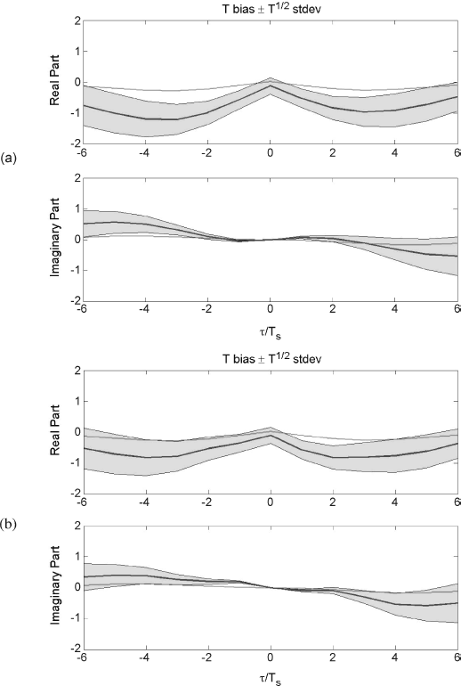
In order to test the dependence on the sampling period T_s of the sample statistics, a second experiment is carried out (see Figure 2.10), where the sampling period T_s = T_p/12 is half that of the previous experiment and (a) N = 2¹² and (b) N = 2¹⁴ data samples are taken in order to obtain the same overall data-record lengths T = NT_s as in cases (a) and (b), respectively, of the first experiment. Similar considerations as for the first experiment hold about the behavior of the normalized sample bias and standard deviation. In particular, according to the theoretical results, the behavior of quantities reported in Figure 2.10 is almost the same as that of those reported in Figure 2.9.

Figure 2.10 Normalized bias of the discrete-time cyclic correlogram as a function of τ/T_s, for , estimated by sampling period T_s = T_p/12 and (a) N = 2¹² and (b) N = 2¹⁴ data samples. Thin line: Normalized (by T) actual value; Thick line: Normalized (by T) estimated value; Shaded area: Normalized (by T^1/2) sample standard deviation.

Source: (Napolitano 2009) © IEEE

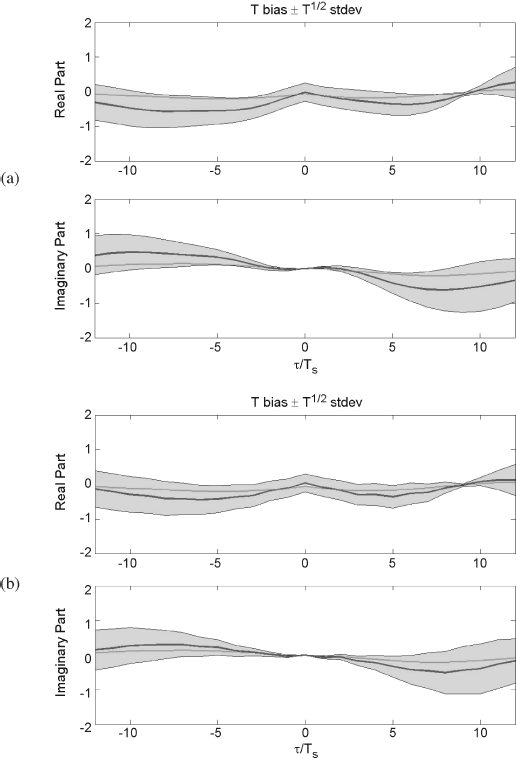
Finally, by comparing the results with the analytic expression of the bias of the continuous-time estimator evaluated by (2.128), the result is that the effect of aliasing is negligible.

2.7.5 Discussion

From Theorems 2.4.11–2.4.13 it follows that the cyclic cross-correlogram is a mean-square consistent estimator of the cyclic cross-correlation function. Such a consistency result does not depend on the knowledge, or not, of the lag-dependent cycle-frequencies α_n(τ). This could appear to contrast with a well-known result valid for (jointly) ACS processes. That is, for ACS processes, if the estimation of the cyclic cross-correlation function has to be performed at a fixed cycle frequency, say α₀, then the not exact knowledge of the value of α₀ leads to a biased estimate. The results established in the chapter do not require the knowledge of the functions α_n(τ) since the estimation of the cyclic cross-correlogram as a function of the two variables (α, τ) is performed. From Theorem 2.4.6, it follows that the expected value of the cyclic cross-correlogram is significantly different from zero within strips of width 1/T around the support curves α = α_n(τ), , of the cyclic cross-correlation function. Thus, in the limit as T→ ∞, the regions of the (α, τ) plane where is significantly different from zero tend to the support curves of the cyclic cross-correlation function, that is, the curves α = α_n(τ), (see (2.39)). If the estimation of the cyclic cross-correlation function has to be performed along a fixed lag-dependent cycle frequency curve α = α_n(τ), that is, a generalized cyclic cross-correlation function has to be estimated, then the not exact knowledge of the function α_n(τ) leads to an asymptotically biased estimate, in accordance with the well-known result for ACS processes. Moreover, in the discrete-time implementation of the estimator, the spacing between adjacent values of in the set should decrease faster than 1/N as N increases.

If the lag-dependent cycle frequencies are unknown, a statistical test for the presence of generalized almost-cyclostationarity can be performed to estimate the unknown functions α_n(τ) by exploiting the asymptotic complex Normality of the cyclic cross-correlogram. A point in the (α, τ) plane belongs to the estimated support if the magnitude of the cyclic cross-correlogram exceeds a threshold whose value has to be fixed in order to find assigned probabilities of false alarm or missed detection.

Note that a different behavior of statistical-function estimators is found for the class of the spectrally correlated stochastic processes (Chapter 4), (Napolitano 2003) that also extend the class of the ACS processes. Spectrally correlated processes have the Loève bifrequency spectrum with spectral masses concentrated on a countable set of curves in the bifrequency plane. The support curves of the Loève bifrequency spectrum play, for spectrally correlated processes, in the frequency domain, a role analogous to that played for GACS processes, in the time domain, by the lag-dependent cycle frequencies. The ACS processes are obtained as a special case of spectrally correlated processes when the separation between correlated spectral components can assume values only in a countable set (which is the set of the cycle frequencies). In such a case, the support curves of the Loève bifrequency spectrum are lines with unit slope. In Chapter 4 it is shown that, for spectrally correlated processes, when the location of the spectral masses is unknown, time-or frequency-smoothed versions of the periodogram do not provide estimates of the bifrequency spectral correlation density function that are asymptotically unbiased and with zero asymptotic variance. Moreover, there exists a tradeoff between the departure of the spectral-correlation-type nonstationarity from the almost cyclostationarity and the reliability of spectral correlation measurements obtainable by a single sample path.

Finally, note that the results of this chapter can be extended to the case in which the second-order cross-moments (2.119) and the fourth-order cumulant (2.120) in Assumption 2.4.2 and the kth-order cumulant (2.164) can be expressed as the sum of an almost-periodic component and a residual term not containing any additive sinewave component (see for example, (2.28b), (2.80a), (2.80b), (2.90a), and (2.90b)), provided that the residual terms are bounded and summable (or at least with finite principal-value integral) with respect to all the variables. For this class of processes, in (Napolitano and Tesauro 2011) continuous-time estimators are proposed for cyclic higher-order statistics.

2.7.6 Conjecturing the Nonstationarity Type of the Continuous-Time Signal

In Section 2.5, it is shown that both ACS and GACS that are not ACS continuous-time signals, by sampling, give rise to ACS discrete-time signals. Thus, the nonstationarity type of the subsumed continuous-time signal cannot be derived from that of the discrete-time signal of its samples. In this section, it is shown how the possible ACS nature of a continuous-time GACS signal can be conjectured from the behavior of the support of the estimated cyclic correlogram of the sampled ACS signal (Izzo and Napolitano 2003, 2005).

Let be the discrete-time process obtained by uniformly sampling with period T_s a continuous-time GACS signal x(t). According to (2.179b) we have

(2.242)

Thus, the support of (in the main cycle frequency domain) is

(2.243)

Let the cyclic correlogram be evaluated by a N-point DFT-based algorithm with zero padding factor P. Thus, the cycle frequency step for the estimator is . Therefore, if the parameters T_s, N, and P are such that the cycle frequency variations within a sampling period are smaller than twice the (normalized) cycle frequency step, that is,

(2.244)

then, due to the interpolation made by the graphic software, the support (2.243) will appear to be continuous in correspondence of the continuous tracts of the functions . Thus, in the case of piecewise constant functions , according to (2.23), the continuous-time signal should be conjectured to be ACS. In contrast, when the are not piecewise constant, the continuous-time GACS signal should be conjectured to be not ACS.

The above-described conjecturing procedure can be found to be inadequate when the relationship involving analysis and signal parameters is not appropriate. In fact, if (2.244) is not satisfied, then the support (2.243) appears discontinuous also in correspondence of the continuous tracts of the functions . Specifically, it is constituted by small constant tracts and, hence, the continuous-time signal should be conjectured to be anyway ACS.

To illustrate how different relationships among analysis and signal parameters can lead to different conjectures on the nonstationarity type of the continuous-time signal, two experiments were conducted. A continuous-time chirp-modulated PAM signal x(t) (see (2.99)) is sampled with period T_s. The PAM signal has full-duty-cycle rectangular pulse, stationary white binary modulating sequence, and symbol period T_p = 8T_s. According to (7.356), the lag-dependent cycle frequencies of x(t) are linear functions with slope γ

(2.245)

where are the cycle frequencies of the PAM signal with rectangular pulse (Gardner 1985), (Gardner et al. 2006). Moreover, according to (7.357), the generalized cyclic autocorrelation functions of x(t) are proportional to the cyclic autocorrelation functions of the PAM signal. From (2.245) it follows

(2.246)

and (2.244) specializes into

(2.247)

The data-record length is T = NT_s with N = 2¹⁰ and the padding factor is P = 1. Therefore, .

In the first experiment, the chirp modulation is with frequency shift ν = 0.02/T_s and chirp rate . Consequently, (2.247) is satisfied and due to the behavior of the support (2.243), x(t) is conjectured to be GACS (Figure 2.11). In the second experiment, ν = 0.02/T_s and . Thus, (2.247) is not satisfied and x(t) is conjectured to be ACS since the support appears as constituted by small constant tracts (Figure 2.12).

Figure 2.11 Chirp-modulated PAM signal. (Top) graph and (bottom) “checkerboard” plot of the magnitude of the cyclic correlogram as a function of αT_s and τ/T_s. The signal is conjectured to be GACS

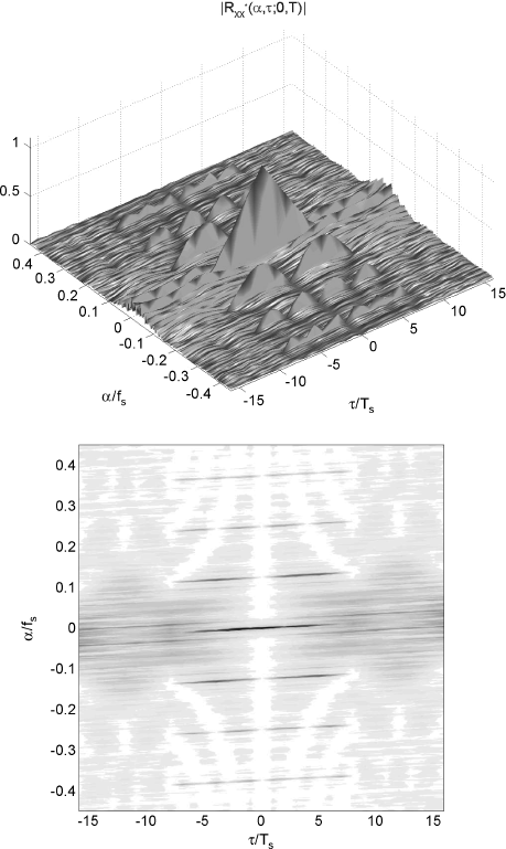
Figure 2.12 Chirp-modulated PAM signal. (Top) graph and (bottom) “checkerboard” plot of the magnitude of the cyclic correlogram as a function of αT_s and τ/T_s. The signal is conjectured to be ACS

Finally, it is worth emphasizing that variations of the (continuous-time) lag-dependent cycle frequencies can be evidenced by finite data-record analysis, provided that the cycle-frequency resolution Δα = 1/T is sufficiently fine, that is, the data-record length T is sufficiently large. For example, let us assume that the lag-dependent cycle frequency is monotone within the interval [τ_a, τ_b]. The cycle-frequency dependence on the lag parameter τ when τ ranges in [τ_a, τ_b] can be appreciated by an observation interval of length T provided that

(2.248)

For the discrete-time estimator, based on N samples, where T = NT_s, condition (2.248) is equivalent to

(2.249)

where and , with , and denoting the floor operation.

In the special case of continuous-time chirp-modulated PAM signal x(t) (see (2.99)), condition (2.248) specializes into

(2.250)

and condition (2.249) into

(2.251)

where , τ_corr is the maximum value of |τ| such that is significantly different from zero, and .

If condition (2.248) is not satisfied , then the lag-dependent cycle frequencies are modeled as constant and the process x(t), on the basis of the data-record length T, is modeled as ACS.

2.7.7 LTI Filtering of GACS Signals

In Section 2.3, it is shown that as a consequence of the input/output relationship (2.117), low-pass or band-pass filtering a purely GACS process leads to a zero power process. In this section, a simulation experiment is conducted aimed at illustrating this result.

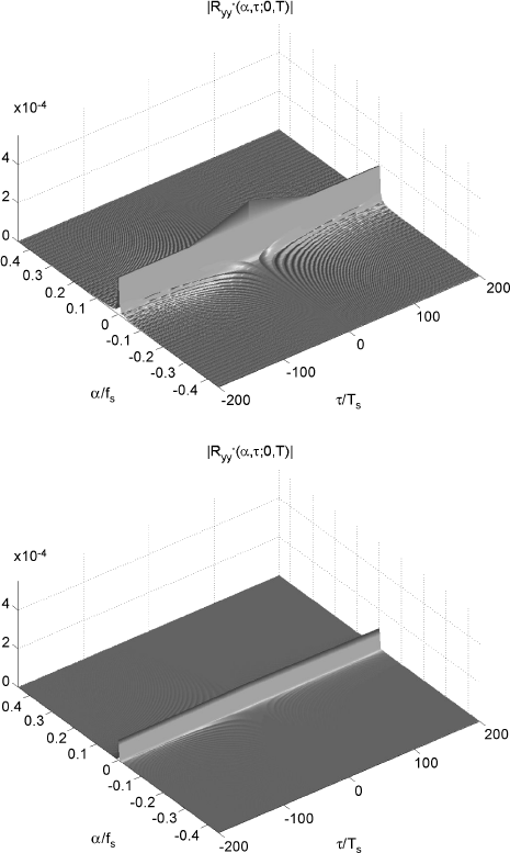
The chirp-modulated PAM signal considered in Section 2.7.6 with chirp rate passes through a low-pass filter with harmonic response H(f) = (1 + jf/B_h)⁻⁴, with B_h = 2 · 10⁻³/T_s. The cyclic correlogram of the output signal y(t) is estimated on observation intervals T = 2⁹T_s (Figure 2.13 (top)) and T = 2¹²T_s (Figure 2.13 (bottom)). The approach of the estimates to the identically zero value as the data-record length increases is evident.

Figure 2.13 LTI filtered chirp-modulated PAM signal. Graph of the magnitude of the cyclic correlogram as a function of αT_s and τ/T_s. (Top) 2⁹ samples and (bottom) 2¹² samples