Chapter 6: Prediction

Being able to predict the future using data is becoming increasingly possible. Not only that; soon, being able to perform successful predictive modeling will not be a competitive advantage anymore—it will be a necessity to survive. To improve the effectiveness of predictive modeling, many focus on the algorithms that are used for prediction; however, there are many meaningful steps you can take to improve the success of prediction by performing more effective data preprocessing. That is the end goal in this book: learning how to preprocess data more effectively. However, in this chapter, we are going to take a very important step toward that goal. In this chapter, we are going to learn the fundamentals of predictive modeling. When we learn the concepts and the techniques of data preprocessing, we will rely on these fundamentals to make better data preprocessing decisions.

While many different algorithms can be applied for predictive modeling, the fundamental concepts of these algorithms are all the same. After covering those fundamentals in this chapter, we will cover two of these algorithms that are distinct from one another in terms of complexity and transparency: linear regression and multi-layer perceptron (MLP).

These are the main topics that this chapter will cover:

• Predictive models
• Linear regression
• MLP

Technical requirements

You will be able to find all of the code and the datasets that are used in this book in a GitHub repository exclusively created for this book. To find the repository, click on this link: https://github.com/PacktPublishing/Hands-On-Data-Preprocessing-in-Python. In this repository, you will find a folder titled Chapter06, from which you can download the code and the data for better learning.

Predictive models

Using data to predict the future is exciting and doable using data analytics. In the realm of data analytics, there are two types of future predictions, outlined as follows:

• Predict a numerical value—for example, predict next year's price of Amazon's stock market.
• Predict a label or a class—for example, predict whether a customer is likely to stop purchasing your services and switch to your competition.

By and large, when we use the term prediction, we mean predicting a numerical value. To predict a class or a label, the term that is used is classification. In this chapter, we will focus on the prediction goal of data analytics, and the next chapter will cover classification.

The prediction of future numerical values also falls into two major overarching types: forecasting and regression analysis. We will briefly explain forecasting, before turning our attention to regression analysis.

Forecasting

In data analytics, forecasting refers to techniques that are used to predict the future numerical values of time-series data. Where forecasting is distinct is in its application to time-series data—for instance, the simplest forecasting method is the simple moving average (SMA). Under this method, you would forecast the numerical value of a future data point in your time-series data using the most recent data points.

Example of using forecasting to predict the future

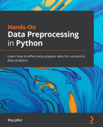
Let's look at an example that features the moving average (MA) for forecasting. The following table shows the number of student applications that Mississippi State University (MSU) received from 2006 to 2021:

Figure 6.1 – Number of MSU applications from 2006 to 2021

The following screenshot visualizes the data presented in the preceding table using a line plot:

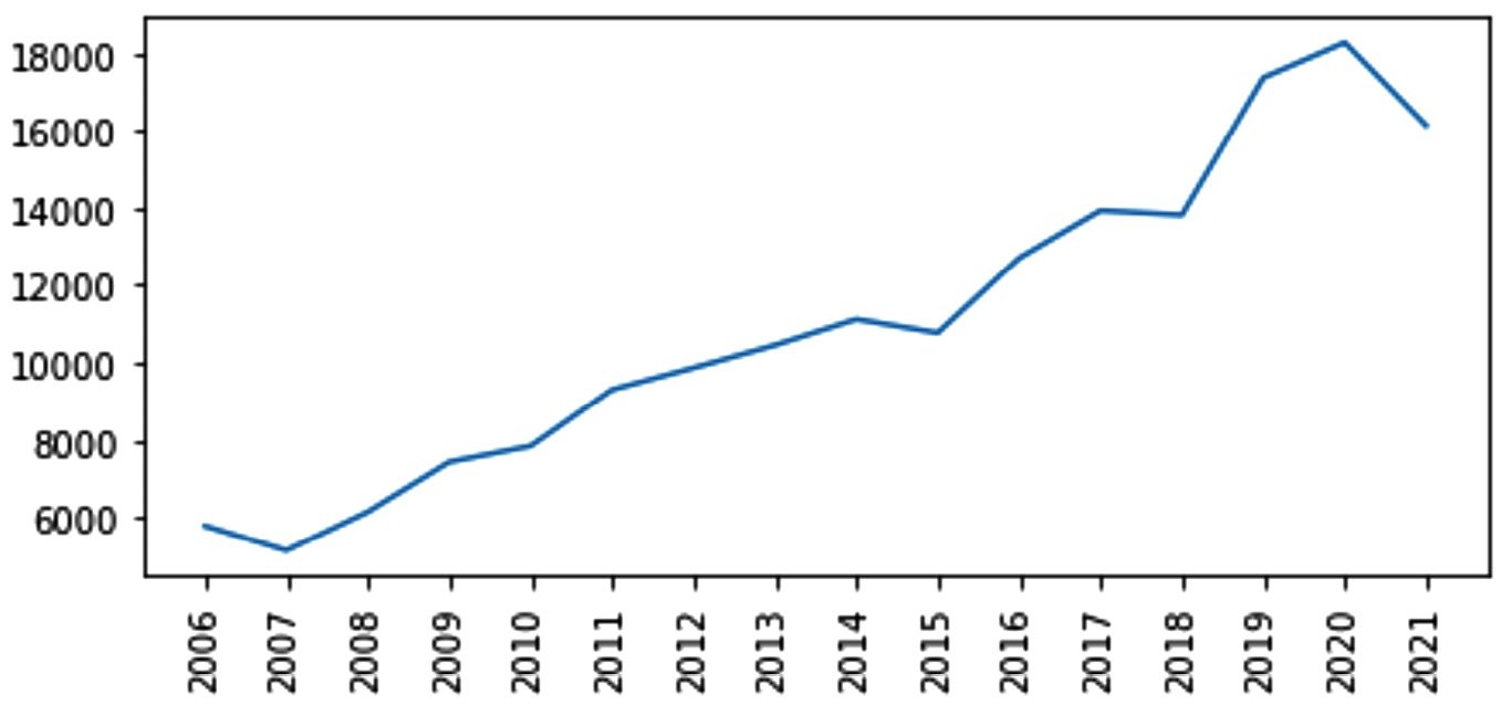
Figure 6.2 – Line plot for the number of MSU applications from 2006 to 2021

MSU, for planning purposes, would like to have some ideas of how many new applications they will receive in 2022. One way to go about this would be to use the MA method. For this method, you need to specify the number of data points you want to use for forecasting. This is often denoted by n. Let's use five data points (n=5). In that case, you would use the data from 2017, 2018, 2019, 2020, and 2021 in your prediction. Simply, you calculate the average number of applications for these years and use that as the estimated forecast for the next year. The average value of 13,930, 13,817, 17,363, 18,269, and 16,127 is 15,901.2, which can be used as an estimate for the number of applications for 2022.

The following screenshot depicts the application of MA with n=5:

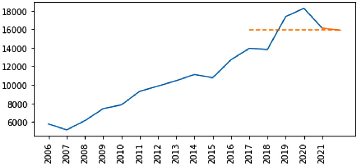
Figure 6.3 – Application of a simple MA forecasting method on the number of MSU applications from 2006 to 2021

There are more complicated methods for forecasting using time-series data such as weighted MA, exponential smoothing, double exponential smoothing, and more.

We do not cover these methods in this book as the data preprocessing that is needed for all time-series data is the same. However, what you'd want to remember from forecasting is that the methods work on single-dimensional time-series data for prediction. For instance, in the MSU example, the only dimension of data we had was the N_Applications attribute.

This single dimensionality is in stark contrast to the next prediction methodology we will cover. Regression analysis, in contrast to forecasting, finds relationships between multiple attributes to estimate numerical values of one of the attributes.

Regression analysis

Regression analysis tackles the task of predicting numerical values using the relationship between predictor attributes and the target attribute.

The target attribute is the attribute whose numerical values we are interested in predicting. The term dependent attribute is another name that is used for the same idea. The meaning of dependent attribute comes from the fact that the value of the target attribute is dependent on other attributes; we call those attributes predictors or independent attributes.

Many different methods could be used for regression analysis. As long as the methods seek to find relationships between the independent attributes and the dependent attribute for predicting the dependent attribute, we categorize the methods under regression analysis. Linear regression, which is one of the simplest and yet widely used methods of regression analysis is, of course, one of these methods. However, other techniques such as MLP and regression tree are also categorized under regression analysis.

Example of designing regression analysis to predict future values

For example, the prediction of the number of MSU applications in the next year can also be modeled using regression analysis. The following figure shows two independent attributes that have the potential to predict the Number of Applications dependent attribute. You can see in this example that the prediction model engages more than one dimension; we have three dimensions—two independent attributes and one dependent attribute.

The first independent attribute, Previous year football performance, is the MSU football team ratio of winning games. The second independent attribute is Average number of applications from last two years:

Figure 6.4 – Example of regression analysis

The second independent attribute is interesting as it depicts that you can interface forecasting methods with regression analysis by including the value of forecasting methods as independent attributes of regression analysis. The average number of applications from the last 2 years is the value of the SMA method with n=2.

How Do We Find Possible Independent Attributes?

You can see the vital role of having appropriate independent attributes for predicting the attribute of interest (dependent attribute) in regression analysis. Envisioning and collecting possible predictors (independent attributes) is the most important part of performing successful regression analysis.

So far, you have learned valuable skills in this book that can help you in the quest to envision possible predictors. The understanding you amassed in Chapter 4, Databases, will allow you to imagine what is possible and search for and collect that data.

In one of the future chapters, Chapter 12, Data Fusion and Integration, you will learn all the skills you will need to go about integrating data from different sources to support your regression analysis.

Once the independent and dependent attributes are identified, we have completed and modeled our regression analysis. Next, we will need to employ the appropriate algorithms to find relationships between these attributes and use those relationships for prediction. In this chapter, we will cover two very different algorithms that can do this: linear regression and MLP.

Linear regression

The name linear regression will tell you all you need to know about it—the regression part tells you this method performs regression analysis, and the linear part tells you the method assumes linear relationships between attributes.

To find a possible relationship between attributes, linear regression assumes and models a universal equation that relates the target (the dependent attribute) to the predictors (the independent attributes). This equation is depicted here:

This equation uses a parameter approach. In this equation N stands for the number of predictors shows the linear regression universal equation.

The working of linear regression is very simple. The method first estimates the βs so that the equation fits the data best, and then uses the estimated βs for prediction.

Let's learn this method with an example. We will continue solving the number of MSU applications in the following example.

Example of applying linear regression to perform regression analysis

We have so far identified our independent and dependent attributes, so we can show the linear regression equation for this example. The equation is shown here:

The MSU applications.csv dataset has all the attributes we need to estimate the βs. Let's first read this data and take a look at it. The following screenshot shows the code we run to read the data and the whole dataset:

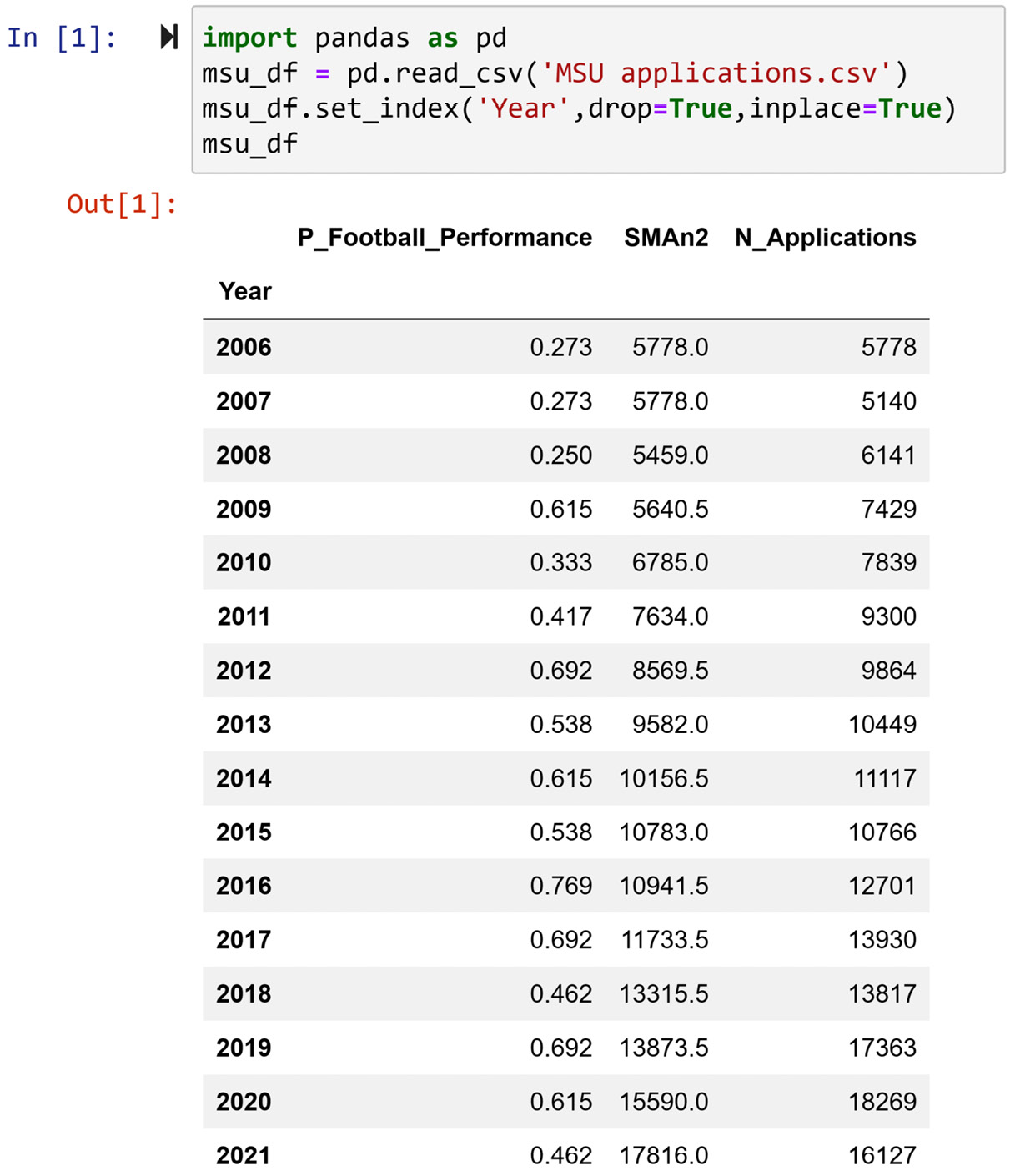
Figure 6.5 – Reading MSU applications.csv and showing the dataset

In this dataset, we have the following attributes:

• P_Football_Performance: This attribute is the overall winning ratio of the MSU football team during the previous academic year.
• SMAn2: This attribute is the calculated value of the SMA with n=2. For instance, SMAn2 for row 2009 is the average of the N_Applications attribute in 2008 and 2007. Confirm this calculation before reading on.
• N_Applications: This is the same data as what we saw in Figure 6.1 and Figure 6.2. This is the dependent attribute that we are interested in predicting.

We are going to use the scikit-learn module to estimate these βs using msu_df, so first, we need to install this module on our Anaconda platform. Running the following code will install the module:

conda install scikit-learn

Once installed, you need to import the module to start using it every time, just as with the other module we have been using. However, since scikit-learn is rather large, we will import exactly what we want to use each time. For instance, the following code only imports the LinearRegression function from the module:

from sklearn.linear_model import LinearRegression

Now, we have at our disposal a function that can seamlessly calculate the βs of our model using msu_df. We now only need to introduce the data to the LinearRegression() function in the appropriate way.

We can do this in four steps, as follows:

1. First, we will specify our independent and dependent attributes, by specifying the X and y list of variables. See the following code snippet:

   X = ['P_Football_Performance','P_2SMA']

   Y = 'N_Applications'

2. Second, we will create two separate datasets from msu_df using the list X and Y: data_X and data_y. data_X is a DataFrame with all the independent attributes, and data_y is a Series that is the dependent attribute. The following code shows this:

   data_X = msu_df[X]

   data_y = msu_df[y]

   This step and the previous step could have been merged with the next steps; however, it is best to keep your code clean and tidy, and I highly recommend using my guidelines, at least in the beginning.

3. Next, we will create the model and introduce the data. The following code will do that. We create a linear regression model and call it lm, and introduce the data to it:

   lm = LinearRegression()

   lm.fit(data_X, data_y)

   When you run the following code almost nothing happens, but don't worry—the model has done its bit, and we only need to access the estimated βs in the next step.

4. As indicated, the estimated βs are within the trained lm model. We can use lm.intercept_ to access β0, and lm.coef_ will show you β1, and β2. The following code prints out an organized report with all the β0 instances:

   print('intercept (b0) ', lm.intercept_)

   coef_names = ['b1','b2']

   print(pd.DataFrame({'Predictor': data_X.columns,                    'coefficient Name':coef_names,                     'coefficient Value': lm.coef_}))

After running these four steps successfully, you will have estimated the βs. I did show the code for this step by step, but all this is normally done in one chunk of code. The following screenshot shows the preceding lines of code and a small report from Step 4:

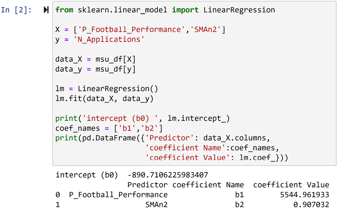
Figure 6.6 – Fitting msu_df data to LinearRegression() and reporting the βs

Now that we have estimated the βs of the regression model, we can introduce our trained model. The following equation shows the trained regression equation:

Next, we will learn how the trained regression equation can be used for prediction.

How to use the trained regression equation for prediction

To use the equation to predict the number of MSU applications in 2022, MSU needs to put together the P_Football_performance and SMAn2 attributes for 2022. Here, we describe the process of finding these values:

• P_Football_performance: At the time of writing this chapter (April 2021), the college football season of 2020-21 had ended and MSU achieved 4 wins out of 11 games, reaching 0.364 winning ratios.
• SMAn2: The N_Applications values for 2021 and 2020 are 18,269 and 16,127, respectively. The average value of these numbers is 17,198.

Here is the calculation to predict N_Applications values in 2022:

We do not have to do the preceding calculations ourselves; we did this for learning purposes. We can use the .predict() function that comes with all of the scikit-learn predictive models. The following screenshot shows how this can be done:

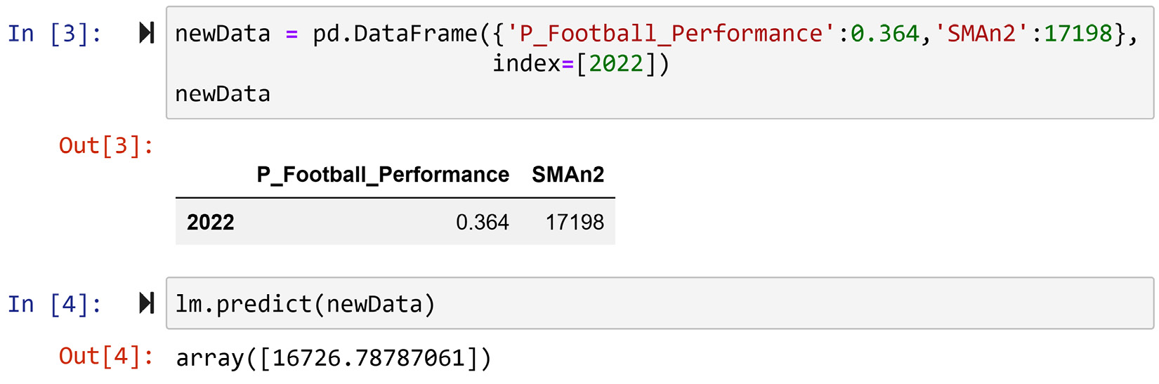
Figure 6.7 – Calculating the number of applications for 2022 using the .predict() function

There is some difference between the preceding equation calculation and programming calculation. One reached 16777.82 and the other arrived at 16726.78. The difference is due to the rounding-ups we did to present the regression equation. The value that the .predict() function came to, 16726.78, is more accurate.

Pay Attention!

Linear regression, and regression analysis in general, is a very established field of analytics. There are many evaluative methods and procedures to ensure the model we have created is of good quality. In this book, we will not cover those concepts, as the goal of this chapter is to introduce techniques that may need data preprocessing. By knowing the mechanism of these techniques, you will be able to perform data preprocessing more effectively.

Now that we have completed this prediction, look back and examine the working of linear regression. Here, linear regression achieved the following two objectives:

1. Linear regression used its universal and linear equation to find the relationship between the independent and dependent attributes. The β coefficient of each independent attribute tells you how the independent attributes relate to the dependent attribute—for instance, the coefficient of SMAn2, β2, came out to be 0.91. This means that even if the MSU football team loses all of its games (which makes the value of N_Football_Performance zero), next year, the number of applications will be an equation of -890.71 + 0.91×SMAn2.
2. The linear regression equation has packaged the estimated relationship in an equation that can be used for future observations.

These two matters, extraction and estimation of the relationships and packaging the estimated relationship for future data objects, are essential for the proper working of any predictive model.

What is great about linear regression is that the simplicity of these matters can be seen and appreciated. This simplicity helps in understanding the working of linear regression and comprehending the patterns it extracts. However, the simplicity works against the method as far as its reach to estimate and package a more complex and non-linear relationship between the independent and dependent attributes.

Next in this chapter, we will be briefly introduced to another prediction algorithm that is at the other end of the spectrum. MLP is a complex algorithm that is capable of finding and packaging more complex patterns between independent and dependent attributes, but it lacks the transparency and intuitiveness of linear regression.

MLP

MLP is a very complex algorithm with many details, and going over its functioning and different parts abstractly will be difficult to follow. So, let's dive in with an example. We will continue using the number of MSU applications in this section.

While linear regression uses an equation, MLP uses a network of neurons to connect the independent attributes to the dependent attribute. An example of such a network is shown in the following screenshot:

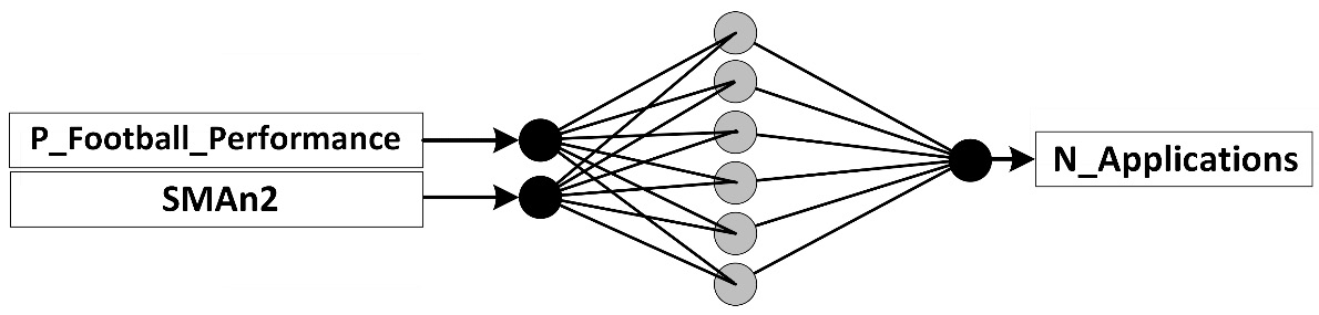
Figure 6.8 – An MLP network example for the number of MSU applications problem

Every MLP network has six distinct parts. Let's go through these parts using Figure 6.8, as follows:

• Neurons: Each of the circles in Figure 6.8 is called a neuron. A neuron could be in the input layer, output layer, and hidden layers. We will cover three tree types of layers in the following section.
• Input layer: A layer of neurons from which values are inputted to the network. In a prediction task, for as many as the number of independent attributes, we will have neurons in the input layer. In Figure 6.8, you can see we have two neurons in the input layer, one for each of our independent attributes.
• Output layer: A layer of neurons out of which the processed values of the network come. In a prediction task, for as many as the number of dependent attributes, we will have neurons in the output layer. More often than not, we only have one dependent attribute. This holds true for Figure 6.8, as our prediction task only has one dependent attribute and the network has only one neuron in the output layer.
• Hidden layers: One or more layers of neurons that come between the input and output layers. The number of hidden layers and the number of neurons in each hidden layer can be—and should be—adjusted for the desired level of model complexity and computational cost. For example, Figure 6.8 only has one hidden layer and six neurons in that hidden layer.
• Connections: The lines that connect the neurons of one layer to the next level are called connections. These connections must exist exhaustively from one level to the next; exhaustively means that all the neurons in a left layer are connected to all the neurons to its right layer.

Now that you understand each part of the preceding MLP network, we will turn our attention to how MLP goes about finding the relationship between the independent attributes and the dependent attribute.

How does MLP work?

MLP works both similarly to and differently from linear regression. Let's first go over their similarities, and then we will cover their differences. Their similarities are listed here:

• Linear regression relies on its structured equation to capture the relationships between the independent attributes and the dependent attribute. MLP, too, relies on its network structure to capture the same relationships.
• Linear regression estimates the βs as a way to use its structured equation to fit itself to the data and hence find the relationship between the independent attributes and the dependent attribute. MLP, too, estimates a value for each of the connections on its structure to fit itself to the data; these values are called the connection's weight. So, both linear regression and MLP use the data to update themselves so that they can explain the data using their predefined structures.
• Once the βs for linear regression and the connections' weight for MLP are properly estimated using the data, both algorithms are ready to be used to predict new cases.

We can see that both algorithms are very similar; however, they also have many differences. Let's go over those now, as follows:

• While the linear regression algorithm's structured equation is fixed and simple, MLP's structure is adjustable and can be set to be very complex. In essence, the more hidden layers and neurons an MLP structure has, the more the algorithm is capable of capturing more complex relationships.
• While linear regression relies on proven mathematical formulas to estimate the βs, MLP has to resort to heuristics and computations to estimate the best connections' weights for the data.

The most famous heuristic that is used to estimate the connections' weights for MLP is called backpropagation. The heuristic is very simple in essence; however, coding it and getting it to work can be tricky. The good news for us is that we do not have to worry about coding it, as there are stable modules we can use. However, let's go through its simple idea once before seeing how we can use the aforementioned modules.

Backpropagation

For backpropagation, each connection's weight is first assigned a random number between -1 and 1. Yes—this is done completely randomly and it is called MLP's random initialization.

After MLP's random initialization, the algorithm will be capable of predicting a value for any inputted data object. Of course, these predictions will be erroneous. Backpropagation uses these errors and the extent of these errors to learn.

Every time a data object is exposed to the MLP network, MLP expects its dependent attribute. As mentioned, this expectation is wrong, at least in the beginning. So, backpropagation calculates the error of the network for each exposure, moves backward on the network, and updates the connection's weight in such a way that if the same data object is exposed again, the amount of error will be a little less.

The network will be exposed to all data objects in the dataset more than once. Every time all the data objects are exposed to the network, we call that one epoch of learning. Backpropagation makes the network undergo enough epochs of learning so that the collective amount of error for the network will be acceptable.

Now that we have this general understanding of MLP and its major heuristic to estimate the connections' weights, let's together see an example of using the scikit-learn module to perform a prediction task using MLP.

Example of applying MLP to perform regression analysis

To implement MLP using the scikit-learn module, we need to take the same four steps that we took for linear regression. In short, these four steps are listed as follows.

1. Specifying our independent and dependent attributes
2. Creating two separate datasets: data_X and data_y
3. Creating a model and introducing the data
4. Predicting

The following code snippet shows these four steps being applied to the number of MSU applications problem. It shows the MLPRegressor class being imported from the sklearn.neural_network module first:

from sklearn.neural_network import MLPRegressor

X = ['P_Football_Performance','SMAn2']

y = 'N_Applications'

data_X = msu_df[X]

data_y = msu_df[y]

mlp = MLPRegressor(hidden_layer_sizes=6, max_iter=10000)

mlp.fit(data_X, data_y)

mlp.predict(newData)

The code is almost the same as the code that we used for linear regression, with some minor changes. Let's go over those, as follows:

• Instead of creating lm using LinearRegression(), we created mlp using MLPRegressor().
• The LinearRegression() function did not need any input, as linear regression is a simple algorithm with no hyperparameters. But MLPRegressor() needed at least two inputs, hidden_layer_sizes=6 and max_iter=10000. The first input (hidden_layer_sizes=6) specifies the network structure. By inputting only one number, we are indicating we only have one hidden layer, and by using the number 6, we are indicating that the hidden layer has six neurons. This is in line with the network design we saw in Figure 6.8. The second input (max_iter=10000) specifies that you want at least 10,000 epochs of learning before the module should give up on converging.

If you successfully run the preceding code a few times, you will observe the following two general trends:

• The code will output a somewhat different prediction for newData every time, but the values are all around 18,000.
• On some runs, the code will also create a warning. The warning is that the MLP algorithm was not able to converge even after 10,000 epochs of learning.

Now, let's discuss these two trends.

MLP reaching different predictions on every run

Let's discuss the first observation: The code will output a somewhat different prediction for newData every time, but the values are all around 18,000.

MLP is a random-based algorithm. If you remember from our backpropagation learning, every time the network is initialized, a random number between -1 and 1 is assigned to each of the connections. These values are then updated so that the network fits the data better; however, the beginning is random, and therefore the results are going to be different.

However, if you pay attention to these different conclusions the random-based model reached, you will see that even though they are different, they are somewhat consistent. They are all around 18,000. This shows that the random-based procedure is capable of finding similar and meaningful patterns in the data.

MLP needing significant epochs of learning

Let's now discuss the second observation: On some runs, the code will also create a warning. The warning is that the MLP algorithm was not able to converge even after 10,000 epochs of learning.

As we will never know when the random-based algorithm will converge, we will have to put a cap on the number of epochs of learning. In fact, having 10,000 epochs of learning is extravagantly high, and we can afford it only because the data has only 16 data objects. The default value of max_iter for MLPRegressor() is 200. That means if we had not specified max_iter=10000, the function would have assumed max_iter=200. In this case, that would mean the algorithm would not converge more often, and its conclusions would be less consistent. Give this a try and observe the aforementioned patterns.

Pay Attention!

MLP is a very complex and flexible algorithm; here, we only discussed two of its hyperparameters (hidden_layer_sizes and max_iter), but it has many more, and to successfully use MLP, you will need to tune it first. To tune an algorithm is to find the hyperparameters that work best for a dataset. We will not cover how MLP is tuned here, as we only need a basic understanding of the algorithm so that it will support our data preprocessing journey.

Furthermore, just as with linear regression, MLP should be rigorously evaluated for validity and reliability before implementation. We will not use those concepts and techniques in this book either for the same reason.

Summary

Congratulations! You made really good progress in this chapter. Together, we learned the fundamental concepts and techniques for using data to perform predictions. We separated the predictions into predicting numerical values and predicting events and labels. In data mining, the term prediction is used for predicting numerical values, and we use classification for predicting events and labels. In this chapter, we covered data mining task prediction, and in the next chapter, we will cover data mining task classification.

Before moving forward and starting your journey to learn about classification and how it can be done in the next chapter, spend some time on the following exercises and solidify your learnings.

Exercises

1. MLP has the potential to create prediction models that are more accurate than prediction models that are created by linear regression. This statement is generally correct. In this exercise, we want to explore one of the reasons why the statement is correct. Answer the following questions:

   a) The following formula shows the linear equation that we used to connect the dependent and independent attributes of the number of MSU applications problem. Count and report the number of coefficients that linear regression can play with to fit the equation to the data.

   

   b) Figure 6.8 shows the MLP network structure we used to connect the dependent and independent attributes of the number of MSU applications problem. Count and report the number of connections' weights MLP can play with to fit the network to the data.

   c) Use your answers from a) and b) to state why MLP has more potential in terms of creating prediction models with higher accuracy.

2. In this exercise, we will be using ToyotaCorolla_preprocessed.csv. This dataset has the following columns: Age, Mileage_KM, Quarterly_Tax, Weight, Fuel_Type_CNG, Fuel_Type_Diesel, Fuel_Type_Petrol, and Price. Each data object in this dataset is a used Toyota Corolla car. We would like to use this dataset to predict the price of used Toyota Corolla cars.

   a) Read the data into the car_df pandas DataFrame.

   b) Use the skills you picked up in the previous chapter to come up with data visualizations that show the relationship between the attribute price and the rest of the attributes.

   c) Use the visuals in b) to describe the relationship each of the attributes has with the attribute price.

   d) Create a correlation matrix for all the attributes, and report the correlation values for the relationship that you investigated in b) and c).

   e) Were the visual investigations you performed in b) and c) confirmed in d)? For which types of attributes were the conclusions for c) not confirmed in d)?

   f) Perform linear regression to predict the attribute price. Use all the attributes that you detect had a meaningful relationship with the attribute price as independent attributes. Predict the price of a car with the following specifications: Age: 74 months, Mileage_KM: 124,057, Quarterly_Tax: 69, and Weight: 1,050. The car fuel type is petrol.

   g) Implement an MLP algorithm to predict the attribute price. Use all the attributes that you used in f) and predict the price of the same new car presented in f). Use 15 neurons in one hidden layer (hidden_layer_sizes), and set the max_iter attribute as 100.

   h) The actual price of the new car presented under f) is 7,950. Report which algorithm performed a better prediction.