Chapter 12: Data Fusion and Data Integration

The popular understanding of data pre-processing goes hand in hand with data cleaning. Although data cleaning is a major and important part of data preprocessing, there are other important areas regarding this subject. In this chapter, we will learn about two of those important areas: data fusion and data integration. In short, data fusion and integration have a lot to do with mixing two or more sources of data for analytic goals.

First, we will learn about the similarities and differences between data fusion and data integration. After that, we will learn about six frequent challenges regarding data fusion and data integration. Then, by looking at three complete analytic examples, we will get to encounter these challenges and deal with them.

In this chapter, we are going to cover the following main topics:

• What are data fusion and data integration?
• Frequent challenges regarding data fusion and integration
• Example 1 (Challenges 3 and 4)
• Example 2 (Challenges 2 and 3)
• Example 3 (Challenges 1, 2, 3, 5, and 6)

Technical requirements

You can find the code and dataset for this chapter in this book's GitHub repository, which can be found at https://github.com/PacktPublishing/Hands-On-Data-Preprocessing-in-Python. You can find chapter12 in this repository and download the code and the data for a better learning experience.

What are data fusion and data integration?

In most cases, data fusion and data integration are terms that are used interchangeably, but there are conceptual and technical distinctions between them. We will get to those shortly. Let's start with what both have in common and what they mean. Whenever the data we need for our analytic goals are from different sources, before we can perform the data analytics, we need to integrate the data sources into one dataset that we need for our analytic goals. The following diagram summarizes this integration visually:

Figure 12.1 – Data integration from different sources

In the real world, data integration is much more difficult than what's shown in the preceding figure. There are many challenges that you need to overcome before integration is possible. These challenges could be due to organizational privacy and security challenges that restrict our data accessibility. But even assuming that these challenges are not in the way when different data sources need to be integrated, they arise because each data source is collected and structured based on the needs, standards, technology, and opinions of the people who have collected them. Regardless of correctness, there are always differences in the ways that the data is structured and because of that, data integration becomes challenging.

In this chapter, we will cover the most frequently faced data integration challenges and learn how to deal with them. These challenges will be discussed in the next subchapter. First, let's understand the difference between data fusion and data integration.

Data fusion versus data integration

As we implied previously, both data integration and data fusion are all about mixing more than one source of data. With data integration, the act of mixing is easier as all the data sources have the same definition of data objects, or with simple data restructuring or transformation, the definitions of the data objects can become the same. When the definitions of the data objects are the same and the data objects are indexed similarly across the data sources, mixing the data sources becomes easy; it will be one line of code. This is what data integration does; it matches the definitions of the data objects across the data sources and then mixes the data objects.

On the other hand, data fusion is needed when the data sources do not have the same definitions as the data objects. With restructuring and simple data transformation, we cannot create the same definitions of data objects across the data sources. For data fusion, we often need to imagine a definition of data objects that is possible for all the data sources and then make assumptions about the data. Based on those assumptions, we must restructure the data sources. So, again, the data sources are in states that have the same definitions of data objects. At that point, the act of mixing the data sources becomes very easy and can be done in one line of code.

Let's try and understand the differences between the two by using two examples: one that needs data integration and one that needs data fusion.

Data integration example

Imagine that a company would like to analyze its effectiveness in how it advertises. The company needs to come up with two columns of data – the total sales per customer and the total amount of advertisement expenditure per customer. As the sales department and marketing department keep and manage their databases, each department will be tasked with creating a list of customers with the relevant information. Once they've done that, they need to connect the data of each customer from the two sources. This connection can be made by relying on the existence of real customers, so no assumptions need to be made. No changes need to be made to connect this data. This is a clear example of data integration. The definition of data objects for both sources is customers.

Data fusion example

Imagine a technology-empowered farmer who would like to see the influence of irrigation (water dispersion) on yield. The farmer has data regarding both the amount of water its revolving water stations have dispensed and the amount of harvest from each point in the farm. Each stationary water station has a sensor and calculates and records the amount of water that is dispensed. Also, each time the blade in the combine harvester moves, the machine calculates and record the amount of harvest and the location.

In this example, there is no clear connection between the sources of data. In the previous example, the clear connection was the definition of data objects - customers. However, we don't have that here, so we need to make assumptions and change the data so that a connection is possible. The situation in this example could look like something like the following figure. The blue dots represent the water stations, while the gray ones represent harvest points:

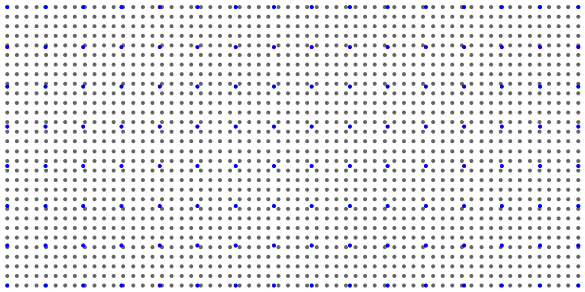
Figure 12.2 – Water points and harvest points

To perform data fusion, we need different sets of assumptions and sets of preprocessing that combine or fuse these data sources. Next, let us see how these assumptions to make the fusion possible may look like.

How about if we defined our data objects as the pieces of land that are harvested? In other words, we define our data objects as harvest points. Then, based on the proximity of the revolving water station to each harvest point, we calculate a number that represents the amount of water the point received. Each water point could be attributed a radius of reach. The closer a harvest point is to the water point within this radius of reach, the more the harvest point got from the amount of water that was dispensed from the water station. We don't know how much water arrives at the harvest points, but we make assumptions about it. These assumptions could be completely naïve or based on some careful experimentation or research.

In this example, we had to come up with a definition of data objects that did not exist within both data sources. Then, we had to make many assumptions about the collected data so that the data sources could be fused.

Good news! You will get to do this data fusion yourself in Exercise 8 at the end of this chapter.

You will see the term data integration for both data integration and data fusion throughout this chapter. When you need to be aware of the distinction between them, the text will inform you of that.

You are almost ready to start seeing the frequent challenges that occur in these areas, as well as some examples, but first, let's discuss one more thing. In the next section, we will introduce two directions of data integration.

Directions of data integration

Data integration may happen in two different directions. The first is by adding attributes; we might want to supplement a dataset with more describing attributes. In this direction, we have all the data objects that we need, but other sources might be able to enrich our dataset. The second is by adding data objects; we might have multiple sources of data with distinct data objects, and integrating them will lead to a population with more data objects that represent the population we want to analyze.

Let's look at two examples to understand the two directions of data integration better.

Examples of data integration by adding attributes

The examples we saw earlier in the Data integration example and Data fusion example sections were both data integration by adding attributes. In these examples, our aim was to supplement the dataset by including more attributes that would be beneficial or necessary for the analytic goals. In both examples, we looked at situations where we would need to perform data integration by adding attributes. Next, we will examine situations that needs data integration by adding data objects.

Examples of data integration by adding data objects

In the first example (Data integration example), we wanted to integrate customer data from the sales and marketing departments. The data objects and customers were the same, but different databases included the data we needed for the analytic goals. Now, imagine that the company has five regional managing bodies and that each managing body is in charge of keeping the data of their customers. In this scenario, data integration will happen after each managing body has come up with a dataset that includes the total sales per customer and the total amount of advertisement expenditure per customer. This type of integration, where we're using five sources of data that include the data of distinct customers, is known as performing data integration by adding data objects.

In the second example (Data fusion example), our goal was to fuse the irrigation and yield data for one piece of land. Regardless of how we would define the data objects to serve the purpose of our analysis, at the end of the day, we will have analyzed only one piece of land. So, different sets of assumptions that would allow the data sources to be fused may have led to different numbers of data objects, but the piece of land stays the same. However, let's imagine that we had more than one piece of land whose data we wanted to integrate. That would become data integration by adding data objects.

So far, we have learned about different aspects of data integration. We have learned what it is and its goals. We've also covered the two directions of data integration. Next, we will learn about the six challenges of data integration and data fusion. After that, we will look at examples that will feature those frequent challenges.

Frequent challenges regarding data fusion and integration

While every data integration task is unique, there are a few challenges that you will face frequently. In this chapter, you will learn about those challenges and, through examples, you will pick up the skills to handle them. First, let's learn about each. Then, through examples that feature one or more of them, we will pick up valuable skills to handle them.

Challenge 1 – entity identification

The entity identification challenge – or as it is known in the literature, the entity identification problem – may occur when the data sources are being integrated by adding attributes. The challenge is that the data objects in all the data sources are the same real-world entities with the same definitions of data objects, but they are not easy to connect due to the unique identifiers in the data sources. For instance, in the data integration example section, the sales department and the marketing department did not use a central customer unique identifier for all their customers. Due to this lack of data management, when they want to integrate the data, they will have to figure out which customer is which in the data sources.

Challenge 2 – unwise data collection

This data integration challenge happens, as its name suggests, due to unwise data collection. For instance, instead of using a centralized database, the data of different data objects is stored in multiple files. We covered this challenge in Chapter 9, Data Cleaning Level I – Cleaning Up the Table, as well. Please go back and review Example 1 – Unwise data collection, before reading on. This challenge could be seen as both level I data cleaning or a data integration challenge. Regardless, in these situations, our goal is to make sure that the data is integrated into one standard data structure. This type of data integration challenge happens when data objects are being added.

Challenge 3 – index mismatched formatting

When we start integrating data sources by adding attributes, we will use the pandas DataFrame .join() function to connect the rows of two DataFrames that have the same indices. To use this valuable function, the integrating DataFrames needs to have the same index formatting; otherwise, the function will not connect the rows. For example, the following figure shows three attempts of combining two DataFrames: temp_df and electric_df. temp_df contains the hourly temperature (temp) of 2016, while electric_df carries the hourly electricity consumption (consumption) for the same year. The first two attempts (the top one and the middle one) are unsuccessful due to the index mismatched formatting challenge. For instance, consider the attempt at the top; while both DataFrames are indexed with Date and Time and both show the same Date and Time, attempting the .join() function will produce a "cannot join with no overlapping index names" error. What is happening? The attempt to integrate was unsuccessful because the index formatting from the two DataFrames is not the same:

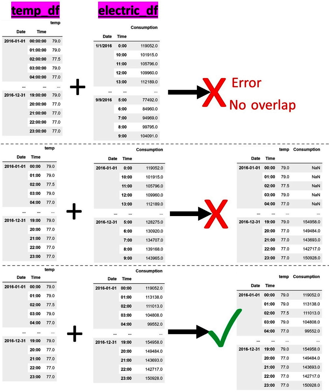
Figure 12.3 – Examples of index mismatched formatting when combining two data sources

In the preceding diagram, while the attempt in the middle is better than the one at the top, it is still unsuccessful. Pay close attention and see if you can figure out why there are so many NaNs in the output of the integration.

Challenge 4 – aggregation mismatch

This challenge occurs when integrating data sources by adding attributes. When integrating time series data sources whose time intervals are not identical, this challenge arises. For example, if the two DataFrames presented in the following figure are to be integrated, not only do we have to address the challenge of index mismatch formatting, but we will also need to face the aggregation mismatch challenge. This is because temp_df carries the hourly temperature data but electric_df carries the electricity consumption of every half an hour:

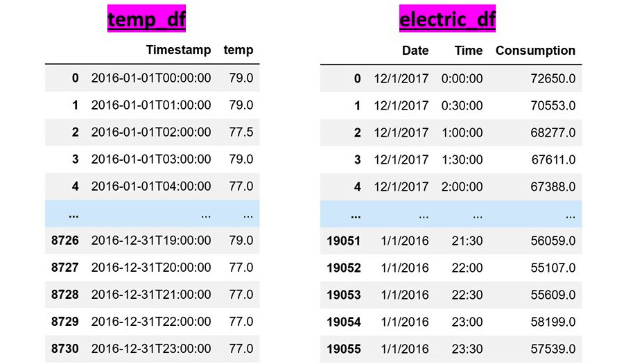
Figure 12.4 – Example of an aggregation mismatch when combining two data sources

To deal with this challenge, we will have to restructure one source or both sources to get them to have the same level of data aggregation. We will see this shortly, so now, let's cover another challenge.

Challenge 5 – duplicate data objects

This challenge occurs when we're integrating data sources by adding data objects. When the sources contain data objects that are also in the other sources, when the data sources are integrated, there will be duplicates of the same data objects in the integrated dataset. For example, imagine a hospital that provides different kinds of healthcare services. For a project, we need to gather the socioeconomic data of all of the patients in the hospital. The imaginary hospital does not have a centralized database, so all of the departments are tasked with returning a dataset containing all the patients they have provided services for. After integrating all of the datasets from different departments, you should expect that there are multiple rows for the patients that had to receive care from different departments in the hospital.

Challenge 6 – data redundancy

This challenge's name seems to be appropriate for the previous challenge as well, but in the literature, the term data redundancy is used for a unique situation. Unlike the previous challenge, this challenge may be faced when you're integrating data sources by adding attributes. As the name suggests, after data integration, some of the attributes may be redundant. This redundancy could be shallow as there are two attributes with different titles but the same data. Or, it could be deeper. In deeper data redundancy cases, the redundant attribute does not have the same title, nor is its data the same as one of the other attributes, but the values of the redundant attribute can be derived from the other attributes.

For example, after integrating data sources into a dataset of customers, we have the following seven attributes: age, average order $, days from the last visit, weekly visit frequency, weekly $ purchase, and satisfaction score. If we use all seven attributes to cluster customers, we have made a mistake regarding data redundancy. Here, the weekly visit frequency, weekly $ purchase, and average order $ attributes are distinct but the value of weekly $ purchase can be derived from weekly visit frequency and average order $. By doing so, inadvertently, we will have given the information regarding the customer's visit and their purchase amount more weight in the clustering analysis.

We should deal with data redundancy challenges that are informed by the analytic goals and data analysis tools. For instance, if we were employing the decision tree algorithm to predict the satisfaction score of the customers, we needn't have worried about data redundancy. This is because the decision tree algorithm only uses the attributes that help its performance.

However, if the same task were to be done using linear regression, you would have a problem if you didn't remove weekly $ purchase. This is because the same information being in more than one attribute would confuse the linear regression. There are two reasons for this:

• First, the linear regression algorithm will have to use all the independent attributes as they are inputted.
• Second, the algorithm needs to come up with a set of weights that works for all the data objects for all the independent attributes, all at the same time. In regression analysis, this situation is referred to as collinearity and it should be avoided.

Now that we've learned about these six common challenges of data integration, let's look at some examples that feature one or some of these challenges.

Example 1 (challenges 3 and 4)

In this example, we have two sources of data. The first was retrieved from the local electricity provider that holds the electricity consumption (Electricity Data 2016_2017.csv), while the other was retrieved from the local weather station and includes temperature data (Temperature 2016.csv). We want to see if we can come up with a visualization that can answer if and how the amount of electricity consumption is affected by the weather.

First, we will use pd.read_csv() to read these CSV files into two pandas DataFrames called electric_df and temp_df. After reading the datasets into these DataFrames, we will look at them to understand their data structure. You will notice the following issues:

• The data object definition of electric_df is the electric consumption in 15 minutes, but the data object definition of temp_df is the temperature every 1 hour. This shows that we have to face the aggregation mismatch challenge of data integration (Challenge 4).
• temp_df only contains the data for 2016, while electric_df contains the data for 2016 and some parts of 2017.
• Neither temp_df nor electric_df has indexes that can be used to connect the data objects across the two DataFrames. This shows that we will also have to face the challenge of index mismatched formatting (challenge 3).

To overcome these issues, we will perform the following steps:

1. Remove the 2017 data objects from electric_df. The following code uses Boolean masking and the.drop() function to do so:

   BM = electric_df.Date.str.contains('2017')

   dropping_index = electric_df[BM].index

   electric_df.drop(index = dropping_index,inplace=True)

   Check the state of electric_df after successfully running the preceding code. You will see that electric_df in 2016 is recorded every half an hour.

2. Add a new column titled Hour to electric_df from the Time attribute. The following code manages to do this in one line of code using the.apply() function:

   electric_df['Hour'] = electric_df.Time.apply(lambda v: '{}:00'.format(v.split(':')[0]))

3. Create a new data structure whose definition of the data object is hourly electricity consumption. The following code uses the .groupby() function to create integrate_sr. The Pandas integrate_sr series is a stopgap data structure that will be used for integration in the later steps:

   integrate_sr = electric_df.groupby(['Date','Hour']).Consumption.sum()

   One good question to ask here is this, why are we using the.sum() aggregate function instead of .mean()? The reason is the nature of the data. The electricity consumption of an hour is the summation of the electricity consumption of its half-hour pieces.

4. In this step, we will turn our attention to temp_df. We will add the Date and Hour columns to temp_df from Timestamp. The following code does this by applying an explicit function:

   First, we will create the function:

   def unpackTimestamp(r):

       ts = r.Timestamp

       date,time = ts.split('T')

       hour = time.split(':')[0]

       year,month,day = date.split('-')

       r['Hour'] = '{}:00'.format(int(hour))

       r['Date'] = '{}/{}/{}'.    format(int(month),int(day),year)

       return(r)

   Then, we will apply the function to the temp_df DataFrame:

   temp_df = temp_df.apply(unpackTimestamp,axis=1)

   Check the status of temp_df after successfully running the preceding code block before moving to the next step.

5. For temp_df, set the Date and Hour attributes as the index and then drop the Timestamp column. The following code does this in one line:

   temp_df = temp_df.set_index(['Date', 'Hour']).drop( columns = ['Timestamp'])

   Again, check the status of temp_df after successfully running the preceding code before moving on to the next step.

6. After all this reformatting and restructuring, we are ready to use .join() to integrate the two sources. The hard part is what comes before using .join(). Applying this function is just as easy as applying it. See for yourself:

   integrate_df =temp_df.join(integrate_sr)

   Note that we came to integrate_sr as a stopgap data structure from Step 3. As always, take a moment to investigate what integrate_df looks like before reading on.

7. Reset the index of integrate_df as we no longer need the index for integration purposes, nor do we need those values for visualization purposes. Running the following code will take care of this:

   integrate_df.reset_index(inplace=True)

8. Create a line plot of the whole year's electricity consumption, where the dimension of temperature is added to the line plot using color. This visualization is shown in Figure 12.5 and was created using the tools we have learned about in this book. The following code creates this visualization:

   days = integrate_df.Date.unique()

   max_temp, min_temp = integrate_df.temp.max(), integrate_df.temp.min()

   green =0.1

   plt.figure(figsize=(20,5))

   for d in days:

       BM = integrate_df.Date == d

       wdf = integrate_df[BM]

       average_temp = wdf.temp.mean()

       red = (average_temp - min_temp)/ (max_temp - min_    temp)

       blue = 1-red

       clr = [red,green,blue]

       plt.plot(wdf.index,wdf.Consumption,c = clr)

   BM = (integrate_df.Hour =='0:00') & (integrate_df.Date.str.contains('/28/'))

   plt.xticks(integrate_df[BM].index,integrate_df[BM].Date,rotation=90)

   plt.grid()

   plt.margins(y=0,x=0)

   plt.show()

   The preceding code brings many parts together to make the following visualization happen. The most important aspects of the code are as follows:

   • The code created the days list, which contains all the unique dates from integrate_df. By and large, the preceding code is a loop through the days list, and for each unique day, the line plot of electricity consumption is drawn and added to the days before and after. The color of each day's line plot is determined by that day's temperature average, that is, temp.mean().
   • The colors in the visualization are created based on the RGB color codes. RGB stands for Red, Green, and Blue. All colors can be created by using a combination of these three colors. You can specify the amount of each color you'd like and Matplotlib will produce that color for you. These colors can take values from 0 to 1 for Matplotlib. Here, we know that when green is set to 0.1, and the red and blue have a blue = 1 - red relationship with one another, we can create a red-blue spectrum of color that can nicely represent hot and cold colors. The spectrum can be used to show hotter and colder temperatures. This has been done by calculating the maximum and minimum of the temperature (using max_temp and min_temp) and calculating the three red, green, and blue elements of clr at the right time to pass as the color value to the plt.plot() function.
   • A Boolean Mask (BM) and plt.xticks() are used to include the 28th of each month on the x axis so that we don't have a cluttered x axis:

Figure 12.5 – Line plot of electricity consumption color-coded by temperature

Now, let's bring our attention to the analytic values shown in the preceding diagram. We can see a clear relationship between temp and Consumption; as the weather becomes colder, the electricity consumption also increases.

We would not be able to draw this visualization without integrating these two data sources. By experiencing the added analytic values of this visualization, you can also appreciate the value of data integration and see the point of having to deal with both Challenge 3 – index mismatched formatting and Challenge 4 – aggregation mismatch.

Example 2 (challenges 2 and 3)

In this example, we will be using the Taekwondo_Technique_Classification_Stats.csv and table1.csv datasets from https://www.kaggle.com/ali2020armor/taekwondo-techniques-classification. The datasets were collected by 2020 Armor (https://2020armor.com/), the first ever provider of e-scoring vests and applications. The data includes the sensor performance readings of six taekwondo athletes, who have varying levels of experience and expertise. We would like to see if the athlete's gender, age, weight, and experience influence the level of impact they can create when they perform the following techniques:

• Roundhouse/Round Kick (R)
• Back Kick (B)
• Cut Kick (C)
• Punch (P)

The data is stored in two separate files. We will use pd.read_csv() to read table1.csv into athlete_df and Taekwondo_Technique_Classification_Stats.csv into unknown_df. Before reading on, take a moment to study athlete_df and unknown_df and evaluate their state to perform the analysis.

After analysis, it will be obvious that the data structure that's been chosen for athlete_df is simple to understand. The data object's definition of athlete_df is athletes, which means that each row represents a taekwondo athelete_df. However, the unknown_df data structure is not readily understandable and is somewhat confusing. The reason for this is that even though a very common data structure – a table – is being used, it is not appropriate. As we discussed in Chapter 3, Data – What Is It Really?, The most universal data structure – a table, we know that the glue that holds a table together is an understandable definition of data objects. Therefore, the major data integration challenge we will face in this example is Challenge 2 – unwise data collection.

To integrate the data when we face unwise data collection challenges, similar to what we did in Chapter 9, Data Cleaning Level I – Cleaning Up the Table, in Example 1 – unwise data collection, we need the data structure and its design to support the following two matters:

• The data structure can include the data of all the files.
• The data structure can be used for the mentioned analysis.

As we've discussed, the athlete_df dataset is simple and easy to understand, but what does the information in unknown_df include? After putting two and two together, we will realize that the sensor readings from the performance of six taekwondo athletes are in athlete_df. From studying unknown_df, we also realize that each athlete has performed each of the four aforementioned techniques five times. These techniques are coded in unknown_df using the letters R, B, C, and P; R stands for roundhouse, B stands for back kick, C stands for cut kick, and P stands for punch. Furthermore, we can see that each technique is performed five times by each athlete.

Running the following code will create an empty pandas DataFrame called performance_df. This dataset has been designed so that both athlete_df and unknown_df can be integrated into it.

The number of rows (n_rows) we have designed for performance_df is one minus the number of columns in unknown_df: len(unknown_df.columns)-1. We will see why that is the case when we are about to fill up performance_df:

designed_columns = ['Participant_id', 'Gender', 'Age', 'Weight', 'Experience', 'Technique_id', 'Trial_number', 'Average_read']

n_rows = len(unknown_df.columns)-1

performance_df = pd.DataFrame(index=range(n_rows),columns =designed_columns)

The following table shows performance_df, which the preceding code creates:

Figure 12.6 – The empty performance_df DataFrame before being filled in

Because the dataset has been collected unwisely, we cannot use simple functions such as .join() for data integration here. Instead, we need to use a loop to go through the many records of unknown_df and athlete_df and fill out performance_df row by row and, at times, cell by cell.

The following pieces of code will use both athlete_df and unknown_df to fill performance_df. Let's get started:

1. First, we need to perform some level I data cleaning for athlete_df so that accessing this DataFrame within the loop becomes easier. The following code takes care of these cleaning steps for athlete_df:

   athlete_df.set_index('Participant ID',inplace=True)

   athlete_df.columns = ['Sex', 'Age', 'Weight', 'Experience', 'Belt']

   Study the state of athlete_df after running the preceding code and make sure that you understand what each line of code does before reading on.

2. Now that athlete_df is cleaner, we can create and run the loop that will fill up performance_df. As shown in the following screenshot, the loop goes through all of the columns in unknown_df. Except for the first column in unknown_df, each column contains information for one of the rows in performance_df. So, in each iteration of looping through the columns of unknown_df, one of the rows of performance_df will be filled. To fill up each row in performance_df, the data must come from both athlete_df and unknown_df. We will use the structures we know about from athlete_df and unknown_df:
   

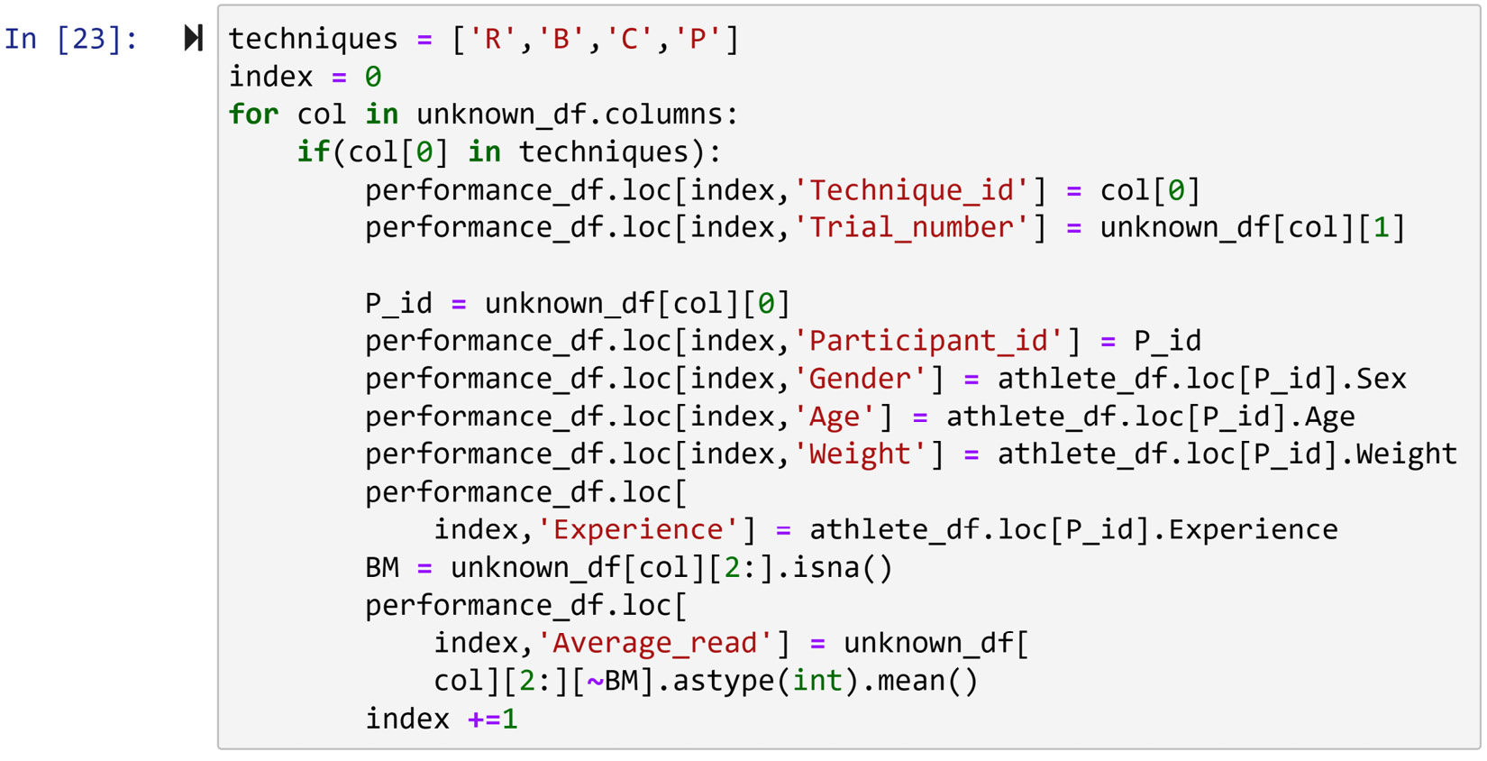
   Figure 12.7 – The code that fills performance_df

   Attention!

   In this chapter, there are going to be a few instances of very large code, such as that shown in the preceding screenshot. Because of the size of this code, we had to include a screenshot instead of a copiable code block. To copy this code, please see the chapter12 folder in this book's GitHub repository.

3. After successfully running the code in the preceding screenshot, performance_df will be filled up. Print performance_df to check its status before reading on.
4. Now that data integration has been performed, we can bring our attention to the data analytic goals. The following code creates a box plot of Average_read based on Gender, Age, Weight, and Experience:

   select_attributes = ['Gender', 'Age', 'Experience', 'Weight']

   for i,att in enumerate(select_attributes):

       plt.subplot(2,2,i+1)

       sns.boxplot(data = performance_df,                y='Average_read', x=att)

   plt.tight_layout()

   plt.show()

   After running the preceding code, the following visualization will be created:

Figure 12.8 – A box plot of Average_read based on Gender, Age, Experience, and Weight

In the preceding diagram, we can see meaningful relationships between Average_read and Gender, Age, Experience, and Weight. In a nutshell, these attributes can change the impact of the techniques that are performed by the athletes. For example, we can see that as the experience of an athlete increases, the impact of the techniques that are performed by the athlete increases.

We can also see a surprising trend: the impact of the techniques that are performed by female athletes is significantly higher than the impact of male athletes. After seeing this surprising trend, let's look back at athlete_df. We will realize that there is only one female athlete in the data, so we cannot count on this visualized trend.

Before we move on to the next data integration example, let's have some fun and create visualizations with higher dimensions. The following code creates multiple box plots that include the Average_read, Experience, and Technique_id dimensions:

sns.boxplot(data = performance_df, y= 'Average_read', x= 'Experience', hue='Technique_id')

The following diagram will be created after running the preceding code:

Figure 12.9 – A three-dimensional box plot of Average_read, Experience, and Technique_id

Before reading on, look at the preceding diagram and see if you can detect more relationships and patterns.

Now, let's bring our attention to the next example. Buckle up – the next example is going to be a complex one with many different aspects.

Example 3 (challenges 1, 3, 5, and 6)

In this example, we would like to figure out what makes a song rise to the top 10 songs on Billboard (https://www.billboard.com/charts/hot-100) and stay there for at least 5 weeks. Billboard magazine publishes a weekly chart that ranks popular songs based on sales, radio play, and online streaming in the United States. We will integrate three CSV files – billboardHot100_1999-2019.csv, songAttributes_1999-2019.csv, and artistDf.csv from https://www.kaggle.com/danield2255/data-on-songs-from-billboard-19992019 to do this.

This is going to be a long example with many pieces that come together. How you organize your thoughts and work in such data integration challenges is very important. So, before reading on, spend some time getting to know these three data sources and form a plan. This will be a very valuable practice.

Now that you've had a chance to think about how you would go about this, let's do this together. These datasets seem to have been collected from different sources, so there may be duplicate data objects among any or all of the three data files. After reading the files into billboard_df, songAttributes_df, and artist_df, respectively, we will check if there are duplicate data objects in them. This is dealing with Challenge 5 – duplicate data objects.

Checking for duplicate data objects

We will have to do this for every file. We will start with billboard_df before doing the same for songAttributes_df and artist_df.

Checking for duplicates in billboard_df

The following code reads the billboardHot100_1999-2019.csv file into Billboard_df and then creates a pandas series called wsr. The name wsr is short for Working SeRies. As I've mentioned previously, I tend to create a wdf (Working DataFrame) or wsr when I need a temporary DataFrame or series to do some analysis. In this case, wsr is used to create a new column that is a combination of the Artists, Name, and Week columns, so we can use it to check if the data objects are unique.

The reason for this multi-column checking is obvious, right? There might be different unique songs with the same name from different artists; every artist may have more than one song; or, the same song may have a different weekly report. So, to check for the uniqueness of the data objects across billboard_df, we need this column:

billboard_df = pd.read_csv('billboardHot100_1999-2019.csv')

wsr = billboard_df.apply(lambda r: '{}-{}-{}'.format(r.Artists,r.Name,r.Week),axis=1)

wsr.value_counts()

After running the preceding code, the output shows that all the data objects appear once except for the song Outta Control by 50 Cent in week 2005-09-14. Running billboard_df.query("Artists == '50 Cent' and Name=='Outta Control' and Week== '2005-09-14'") will filter out these two data objects. The following screenshot displays the outcome of running this code:

Figure 12.10 – Filtering the duplicates in bilboard_df

Here, we can see that the two rows are almost identical and that there is no need to have both of them. We can use the.drop() function to delete one of these two rows. This is shown in the following line of code:

billboard_df.drop(index = 67647,inplace=True)

After running the preceding line of code successfully, it seems that nothing has happened. This is due to inplace=True, which makes Python update the DataFrame in place instead of outputting a new DataFrame.

Now that we are certain about the uniqueness of each row in bilboard_df, let's move on and do the same thing for songAttributes_df.

Checking for duplicates in songAttributes_df

We will use a very similar code and approach to see if there are any duplicates in songAttributes_df. The following code has been altered for the new DataFrame.

First, the code reads the songAttributes_1999-2019.csv file into songAttributes_df, then creates the new column and checks for the duplicates using .value_counts(), which is a function of every pandas Series:

songAttribute_df = pd.read_csv('songAttributes_1999-2019.csv')

wsr = songAttribute_df.apply(lambda r: '{}---{}'.format(r.Artist,r.Name),axis=1)

wsr.value_counts()

After running the preceding code, we will see that many songs have duplicate rows in songAttributes_df.

We need to find out the causes of these duplicates. We can filter out the duplicates of a few songs and study them. For instance, from the top, we can run the following lines of codes separately to study their output:

• songAttribute_df.query("Artist == 'Jose Feliciano' and Name == 'Light My Fire'")
• songAttribute_df.query("Artist == 'Dave Matthews Band' and Name == 'Ants Marching - Live'")

After studying the output of these codes, we will realize that there are two possible reasons for the existence of duplicates:

• First, there might be different versions of the same song.
• Second, the data collection process may have been done from different resources.

Our study also shows that the attributes' value of these duplicates, while not identical, are very similar.

To be able to do this analysis, we need to have only one row for each song. Therefore, we need to either remove all but one row for the songs with duplicates or aggregate them. Either might be the right course of action, depending on the circumstances. Here, we will drop all the duplicates except for the first one. The following code loops through the songs with duplicate data objects in songAttributes_df and uses .drop() to delete all the duplicate data objects, except for the first one. First, the code creates doFrequencies (do is short for data object), which is a pandas series that shows the frequencies of each song in songAttributes_df, and loops through the elements of doFrequencies whose frequency is higher than 1:

songAttribute_df = pd.read_csv('songAttributes_1999-2019.csv')

wsr = songAttribute_df.apply(lambda r: '{}---{}'.format(r.Name,r.Artist),axis=1)

doFrequencies = wsr.value_counts()

BM = doFrequencies>1

for i,v in doFrequencies[BM].iteritems():

    [name,artist] = i.split('---')

    BM = ((songAttribute_df.Name == name) & (songAttribute_    df.Artist == artist))

    wdf = songAttribute_df[BM]

    

    dropping_index = wdf.index[1:]

    songAttribute_df.drop(index = dropping_index, inplace=True)

If you try running the preceding code, you will see that it will take a long time. It took around 30 minutes on my computer. In these situations, it is nice to add some elements to the code that give users some idea of how much the code has run and how much more time will be needed. The following code is the same as the preceding one, but some more elements have been added to create a mechanism for reporting the progress of the runtime. I would suggest running the following code instead. But before doing so, compare the two options and study how the reporting mechanism is added. Do not forget that you will need to import the time module before you can run the following code. The time module is an excellent module that allows us to work with time and time differences:

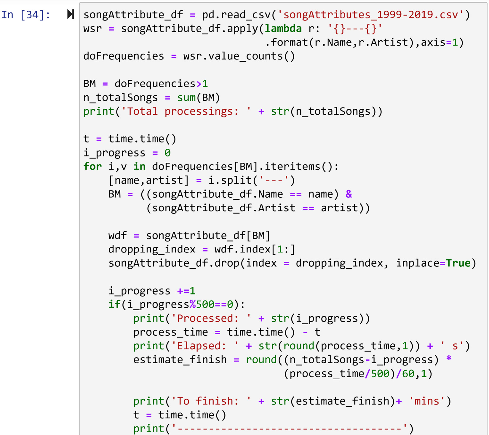
Figure 12.11 – Dropping the duplicates that were added with code to report progress

Once you've successfully run the preceding code, which will take a while, songAttributes_df will not suffer from duplicate data object problems.

Next, we will check if artist_df contains duplicates and address them if it does.

Checking for duplicates in artist_df

Checking the uniqueness of the data objects in artisit_df is easier than it was for the two DataFrames we looked at previously. The reason for this is that there is only one identifying column in artist_df. There were two and three identifying columns for songAttribute_df and billboard_df.

The following code reads artistDf.csv into artisit_df and uses the .value_counts() function to check if all the rows in artisit_df are unique:

artist_df = pd.read_csv('artistDf.csv')

artist_df.Artist.value_counts()

After running the preceding code and studying its results, you will see that two rows represent the artist Reba McEntire. Running artist_df.query("Artist == 'Reba McEntire'") will filter out these two rows. The following screenshot displays the outcome of running this code:

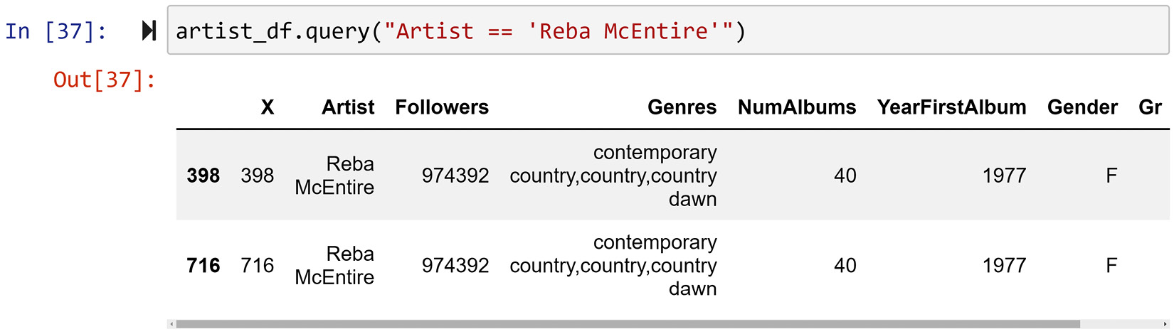
Figure 12.12 – Filtering the duplicates in artist_df

Here, we can see that the two rows are the same and that there is no need to have both of them. The following line of code uses the .drop() function to delete one of these two rows:

artist_df.drop(index = 716, inplace=True)

After running the preceding line of code successfully, it seems that nothing has happened. This is due to inplace=True, which makes Python update the DataFrame in place instead of outputting a new DataFrame.

Well done! Now, we know that all of our DataFrames only contain unique data objects. We can use this knowledge to tackle the challenging task of data integration.

We are better off if we start with the end in sight. In the next section, we will envision and create the structure of the DataFrame we would like to have at the end of the data integration process.

Designing the structure for the result of data integration

As there are more than two data sources involved, it is paramount that we have a vision in sight for the result of our data integration. The best way to do this is to envision and create a dataset whose definition of data objects and its attribute have the potential to answer our analytic questions and, at the same time, can be filled by the data sources that we have.

The following screenshot shows the code that can create a dataset that contains the listed characteristics. The definition of the data objects is songs, while the attributes can be filled in using one of three DataFrames. Once songIntegrate_df has been filled, it can help us answer the question of what makes a song go all the way up to the top 10 on Billboard and stay there for at least 5 weeks:

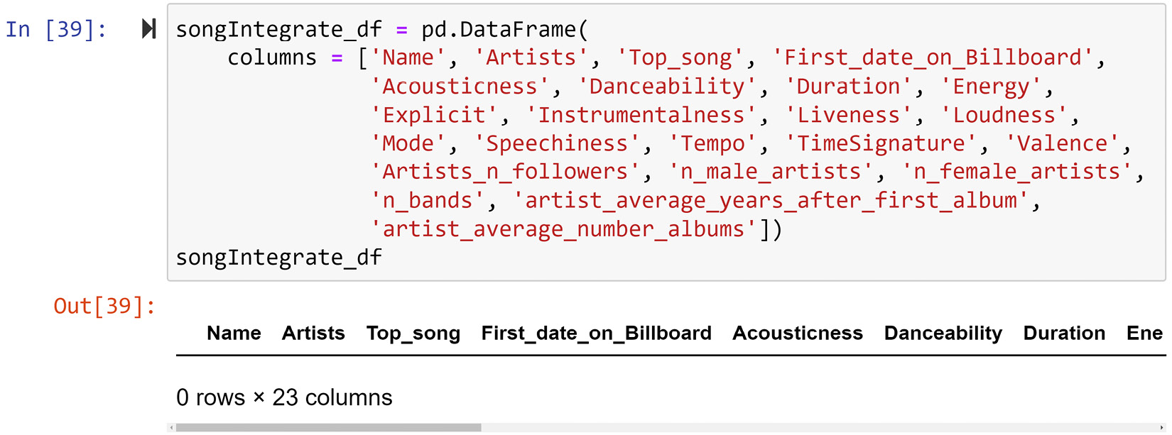
Figure 12.13 – Designing and creating the result of data integration for songIntegrate_df

Most of the envisioned attributes in songIntegrate_df are intuitive. Let's go over the ones that might not be as obvious:

• Top_song: A binary attribute that describes if the song has been in the top 10 songs of Billboard for at least 5 weeks.
• First_date_on_Billboard: The first date that the song was on Billboard.
• Acousticness, Danceability, Duration, Energy, Explicit, Instrumentalness, Liveness, Loudness, Mode, Speechiness, Tempo, TimeSignature, and Valence are the artistic properties of songs. These attributes will be integrated into songIntegrate_df from songAttribute_df.
• Artists_n_followers: The artist's or artists' number of followers on social media. If there is more than one artist, the summation of their number of followers will be used.
• n_male_artists and n_female_artists are the attributes that show the gender of the artists. If one female artist has produced the song, their values will be 0 and 1, respectively. If two male artists have produced the song, their values will be 2 and 0, respectively.
• n_bands: The number of bands that have been involved in producing the song.
• artist_average_years_after_first_album tries to capture the experience of the artists in the business. If one artist has created the song, then a single value will be used, and when more than one artist is involved, an average value is used. These values will be calculated based on First_date_on_Billboard.
• artist_average_number_albums also attempts to capture the experience of the artists in the business. Similar to the previous attribute, if one artist has created the song, then a single value will be used, while when more than one artist is involved, an average value will be used.

The first four attributes will be filled using billboard_df, the last six attributes will be filled using artist_df, and the rest will be filled using songAttribute_df.

Note that the First_date_on_Billboard attribute will be created temporarily. It will be filled from billboard_df so that when we get around to filling from artist_df, we can use First_date_on_Billboard to calculate artist_average_years_after_first_album.

Before we start filling up songIntegrate_df from the three sources, let's go over the possibility of having to remove some songs from songIntegrate_df. This might become inevitable because the information we may need for every song on file may not exist in the other resource. Therefore, the rest of the subsections in this example will be as follows:

• Filling songIntegrate_df from billboard_df
• Filling songIntegrate_df from songAttribute_df
• Removing data objects with incomplete data
• Filling songIntegrate_df from artist_df
• Checking the status of songIntegrate_df
• Performing the analysis

It seems that we've got a lot of ground to cover, so let's get to it. We will start by using billboard_df to fill songIntegrate_df.

Filling songIntegrate_df from billboard_df

In this part of filling songIntegrate_df, we will be filling the first four attributes: Name, Artists, Top_song, and First_date_on_Billboard. Filling the first two attributes is simpler; the latter two need some of the rows in billboard_df to be calculated and aggregated.

The challenge of filling data from billboard_df into songIntegrate_df is two-fold. First, the definitions of the data objects in the two DataFrames are different. We have designed the definition of the data objects in songIntegrate_df to be songs, while the definition of the data objects in billboard_df is the weekly reports of songs' billboard standings. Second, as billboard_df has a more complex definition of data objects, it will also need more identifying attributes to distinguish between unique data objects. For billboard_df, the three identifying attributes are Name, Artists, and Week, but for songIntegrate_df, we only have Name and Artists.

The songIntegrate_df DataFrame is empty and contains no data objects. Since the definition of data objects we have considered for this DataFrame is songs, it is best to allocate a new row in songIntegrate_df for all the unique songs in billboard_df.

The following code loops through all the unique songs in billboard_df using nested loops to fill songIntegrate_df. The first loop goes over all the unique song names, so each iteration will be processing one unique song name. As there might be different songs with the same song name, the code does the following within the first loop:

1. First, it will filter all the rows with the song name of the iteration.
2. Second, it will figure out all Artists who have had a song with the song name of the iteration.
3. Third, it will go over all Artists we recognized in the second step and as per each iteration of this second loop, we will add a row to songIntegrate_df.

To add a row to songIntegrate_df, the following code has used the.append() function. This function either takes a pandas Series or a Dictionary to add it to a DataFrame. Here, we are using a dictionary; this dictionary will have four keys, which are the four attributes – Name, Artists, Top_song, First_date_on_Billboard – of songIntegrate_df that we intend to fill from billboard_df. Filling Name and Artists is easy as all we need to do is insert the values from billboard_df. However, we need to make some calculations to figure out the values of Top_song and First_date_on_Billboard.

Study the following code and try to understand the logic behind the parts of the code that try to calculate these two attributes. For Top_song, try to see if you can connect the logic to what we are trying to do. Go back to the very first paragraph in this example. For First_date_on_Billboard, the code has assumed something about billboard_df. See if you can detect what that assumption is and then investigate if that assumption is reliable.

Now, it is time for you to give the code a try. Just a heads-up before you hit run: it might take a while to finish. It will not be as lengthy as the preceding code to run, but it won't be instantaneous either:

SongNames = billboard_df.Name.unique()

for i, song in enumerate(SongNames):

    BM = billboard_df.Name == song

    wdf = billboard_df[BM]  

    Artists = wdf.Artists.unique()

    for artist in Artists:

        BM = wdf.Artists == artist

        wdf2 = wdf[BM]

        topsong = False

        BM = wdf2['Weekly.rank'] <=10

        if(len(wdf2[BM])>=5):

            topsong = True

        first_date_on_billboard = wdf2.Week.iloc[-1]

        dic_append = {'Name':song,'Artists':artist, 'Top_        song':topsong, 'First_date_on_Billboard': first_date_        on_billboard}

        

        songIntegrate_df = songIntegrate_df.append(dic_append,         ignore_index=True)

After successfully running the preceding code, print songIntegrate_df to study the state of the DataFrame.

The challenge we just faced and addressed here can be categorized as Challenge 3 – index mismatched formatting. This particular challenge is more difficult as not only do we have different index formatting but also we have different definitions of data objects. To be able to perform data integration, we had to refrain from declaring the identifying attributes as indexes. Why? Because that would not help our data integration goal. However, having to do that also forced us to take things into our hands and use loops instead of simpler functions such as .join(), as we saw in Example 1 (challenges 3 and 4) and Example 2 (challenges 2 and 3).

Next, we will fill in some of the remaining attributes of songIntegrate_df from songAttribute_df. Doing this will challenge us somewhat differently; we will have to deal with Challenge 1 – entity identification.

Filling songIntegrate_df from songAttribute_df

The challenge we have to reckon with in this part of data integration is entity identification. While the definitions of the data objects for both songIntegrate_df and songAttribute_df are the same – that is, songs – the way the unique data objects are distinguished in the two DataFrames is different. The crux of the difference goes back to the songIntegrate_df.Artists and songAttribute_df.Artist attributes; pay attention to the plural of Artists and the singular of Artist. You will see that the songs that have more than one artist are recorded differently in these two DataFrames. However, in songIntegrate_df, all of the artists of a song are included in the songIntegrate_df.Artists attribute, separated by commas (,); in songAttribute_df, only the main artist is recorded in songAttribute_df.Artist and if other artists are involved in a song, they are added to songAttribute_df.Name. This makes identifying the same songs from the two DataFrames very difficult. So, we need to have a plan before we approach data integration here.

The following table shows the five different situations where the same songs entered our two sources. Let's answer two questions about these five situations.

First, how did we come up with these five situations? That is an excellent question. When dealing with the entity identification challenge, you will need to study the sources of the data and figure out how to work with the identifying attributes in the sources. Then, you can use a computer to connect the rows that are for the same entity but not coded the same way. So, the answer to this question is that we just studied the two sources enough to realize that these five situations exist.

Second, what do we do with these situations? Answering this question is simple. We will use them to draft some code that will connect the identifiable songs from both sources to connect and integrate the datasets:

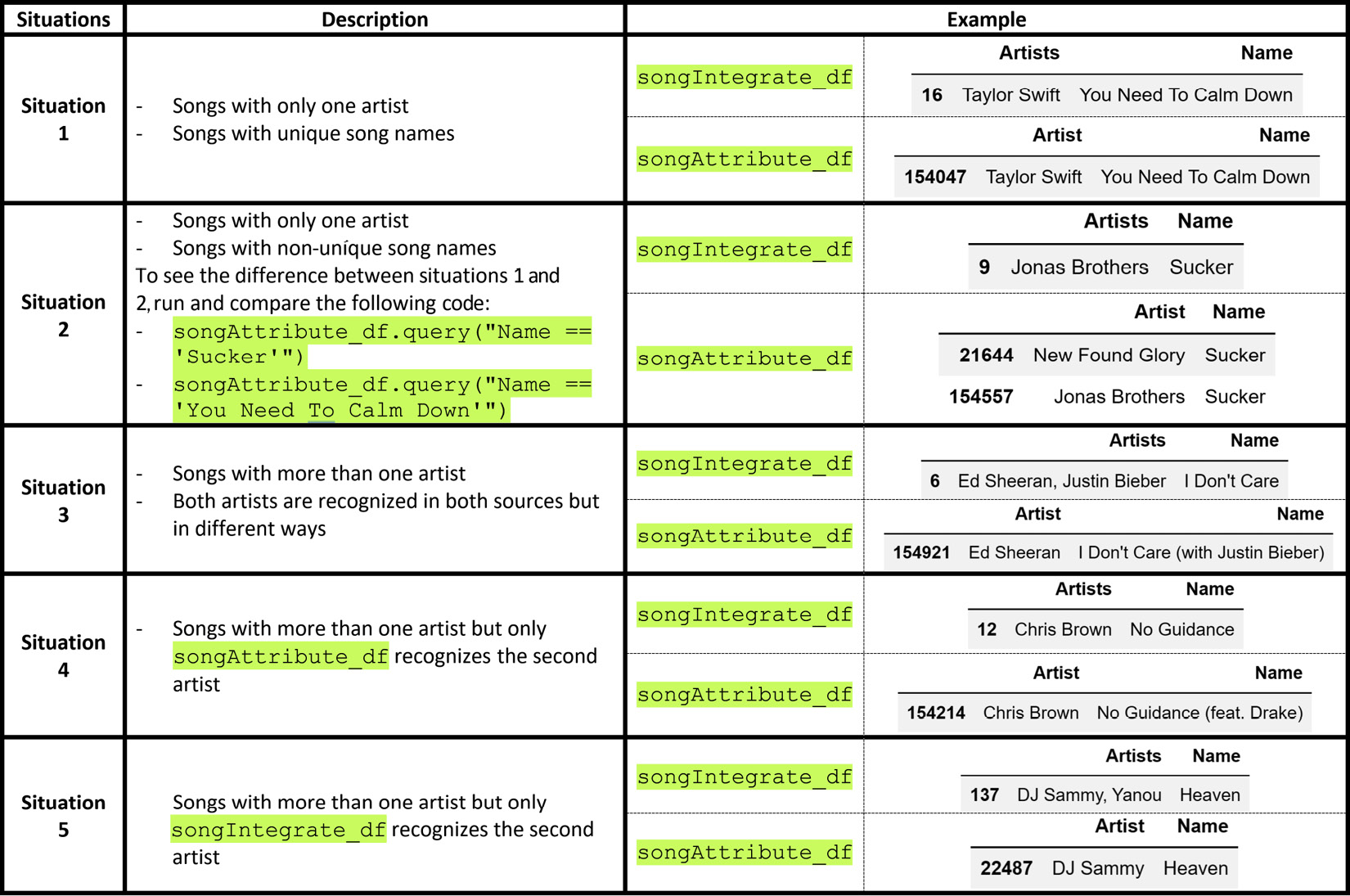
Figure 12.14 – Five situations in the integration of songIntegrate_df with songAttribute_df due to the entity identification challenge

The following code, which is rather long, uses the five extracted situations from the preceding diagram and all the other coding capabilities we've picked up in this book to perform the integration task. The code loops through the rows of songIntegrate_df and searches for any rows in songAttribute_df that have listed the song. The code employes the five situations we've extracted to create the preceding diagram as a guideline to search for songAttribute_df.

Before you look at the following code, allow me to bring your attention to a quick matter. Since the code is lengthy, it's been commented to help you decipher it. Python line comments can be created using #, so, for example, when you see # Situation 1, that means what's coming has been created by our understanding of situation 1.

Now, spend some time using the preceding diagram and the code in the following screenshot to understand how the connection between songIntegrate_df and songAttribute_df has been made:

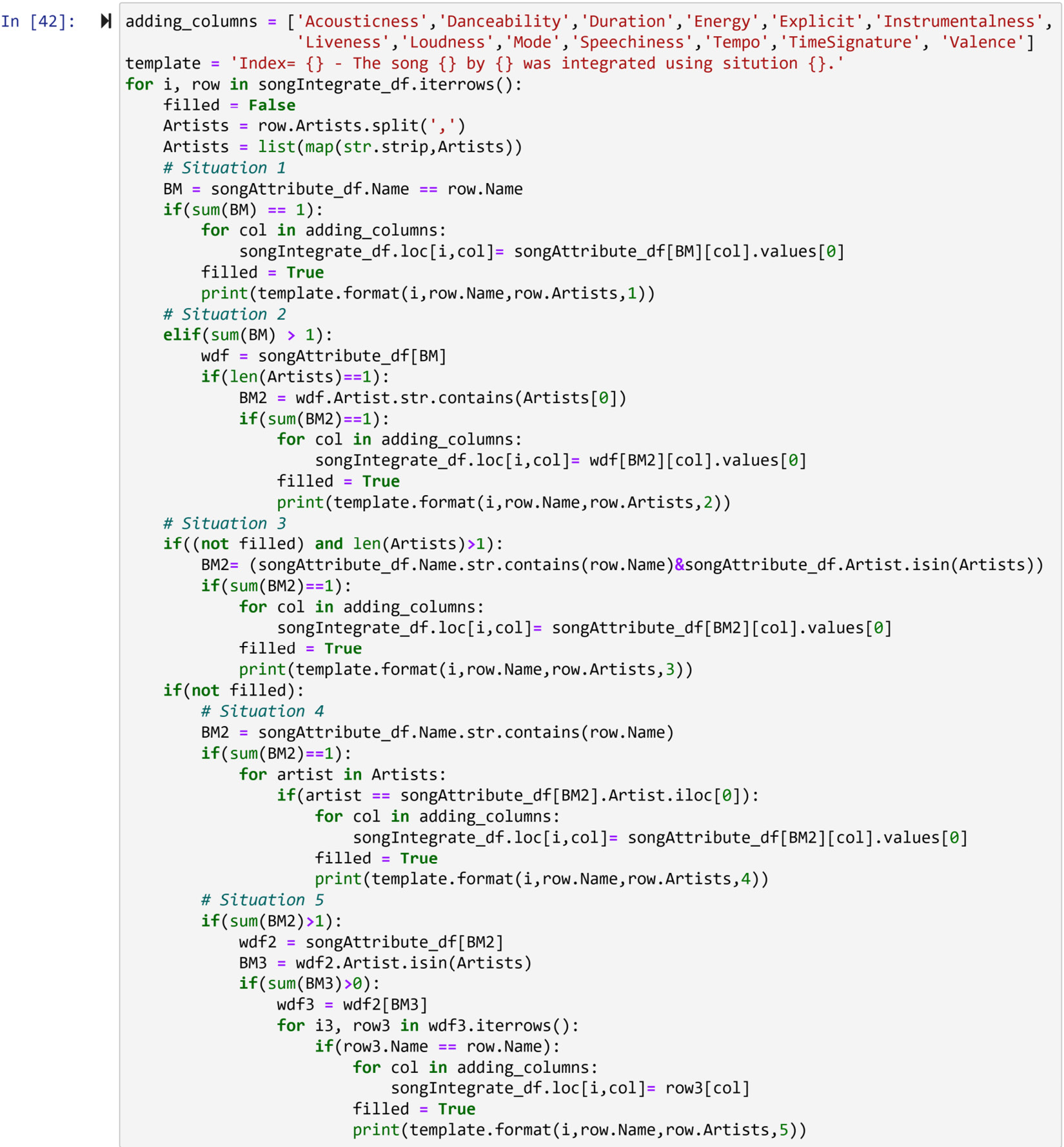
Figure 12.15 – Creating the connection between songIntegrate_df and songAttribute_df

After successfully running the preceding code, which might take a while, spend some time studying the report it provided. If you have paid attention, then you'll know that the code is printed out every time a connection between songs is found. This also happens if the connection was possible. Study the printout to see the frequencies of the situations. Answer the following questions:

• Which situation was the most frequent?
• Which situation was the least frequent?
• Were all of the rows in songIntegrate_df filled in with the values found in songAttribute_df?

The answer to the last question is no – running songIntegrate_df.info() will only show you that 4,045 out of 7,213 rows were filled from songAttribute_df. A critical question to answer regarding this data not being filled completely is to see if there is meaningful discrimination between the top songs and not the top song. If there is any meaningful discrimination, then the values listed in songAttribute_df become much less valuable. This is because our goal is to study the impact that the song attributes have on the song becoming a top song. So, let's study this before moving on to the next filling.

The following screenshot shows the contingency table for the two binary variables, songIntegrate_df.Top_song, and the missing values. It also shows the p-value of the chi-square test of association:

Figure 12.16 – The code and their output for studying if missing values in songIntegrate_df after integrating with songAttribute_df are meaningfully connected to songIntegrate_df.Top_song

After studying the preceding screenshot, we can conclude that there is not enough evidence for us to reject the hypothesis that the missing values don't have a relationship with the songs being a top song or not.

This makes our job easier as we won't need to do anything but remove the rows that don't contain values before we start using artist_df to fill songIntegrate_df. The following code uses the .drop() function to delete the rows in songIntegrate_df that songAttribute_df failed to fill. Note that the B_MV variable comes from the code in the preceding screenshot:

dropping_index = songIntegrate_df[B_MV].index

songIntegrate_df.drop(index = dropping_index,inplace=True)

Successfully running the preceding code and before moving on to the next step, which is using artist_df to fill the rest of songIntegrate_df, run songIntegrate_df.info() to evaluate the state of the DataFrame and ensure that the drops went as planned.

Filling songIntegrate_df from artist_df

The last six attributes of songIntegrate_df, which are Artists_n_followers, n_male_artsits, n_female_artsits, n_bands, artist_average_years_after_first_album, and artist_average_number_albums, will be filled from artist_df. The entity identification challenge that we face here is much simpler than what we did when integrating songIntegrate_df and songAttribute_df. The definitions of the data objects in artist_df are artists, and that is only one part of the definition of the data objects in songIntegrate_df. All we need to do is find the unique artist or artists of each song of songIntegrate_df in artist_df and then fill in songIntegrate_df.

All of the attributes we need to fill in here need information from artist_df, but there will be no direct filling. All of the aforementioned attributes will need to be calculated using the information from artist_df.

Before data integration is possible, we will need to perform one pre-processing task on artist_df. We need to make artist_df searchable by the name of the artist; that is, we must set the index of artist_df as Artist. The following line of code makes sure that happens. The following code also drops the X column, which will not serve any purpose at this point:

artist_df = artist_df.set_index('Artist').drop(columns=['X'])

Now, before moving on to the data integration part, give the searchable artist_df a chance to show you how easy it can gather the information of each artist. For example, try artist_df.loc['Drake'] or any other artist you may know of.

The code in the following screenshot loops through all the rows of songIntegrate_df to find the needed information about the songs' artists and fill up the last six attributes of songIntegrate_df. In each iteration, the code separates the artists of the songs in songIntegrate_df and checks if artists_df contains the information of all of the song's artists. If not, the code terminates as there is not enough information in artist_df to fill out the six attributes. If this information exists, the code assigns zero to all six new attributes and then, within some conditional and logical calculations, updates the zero values.

Before you get your teeth into this rather large piece of code, a few words of caution. First, the lines of code are rather long, so they may have been cut into more than one line. There are two different ways to cut a line of code into more lines. The better method is called implicit line continuation; whenever the line breaks after a parenthesis, (, a curly brace, {, or square bracket, [, Python assumes there is more to come and automatically goes to the next line while looking for it. The other method – the one we try to avoid if we can – is known as explicit line continuation and is where Python will not go looking for more in the next line unless we explicitly request this by using a backslash, , at the end of the line.

The second word of caution is that the code uses what is called augmented arithmetic assignment to save space when writing code. These types of assignments are used to avoid writing the same variable twice when the calculation of the new value of the variable involves the old value of the variable. For instance, you can write x+=1 instead of x = x +1, or you can write y/=5 instead of y = y/5. Augmented arithmetic assignment has been used in multiple places throughout the following code:

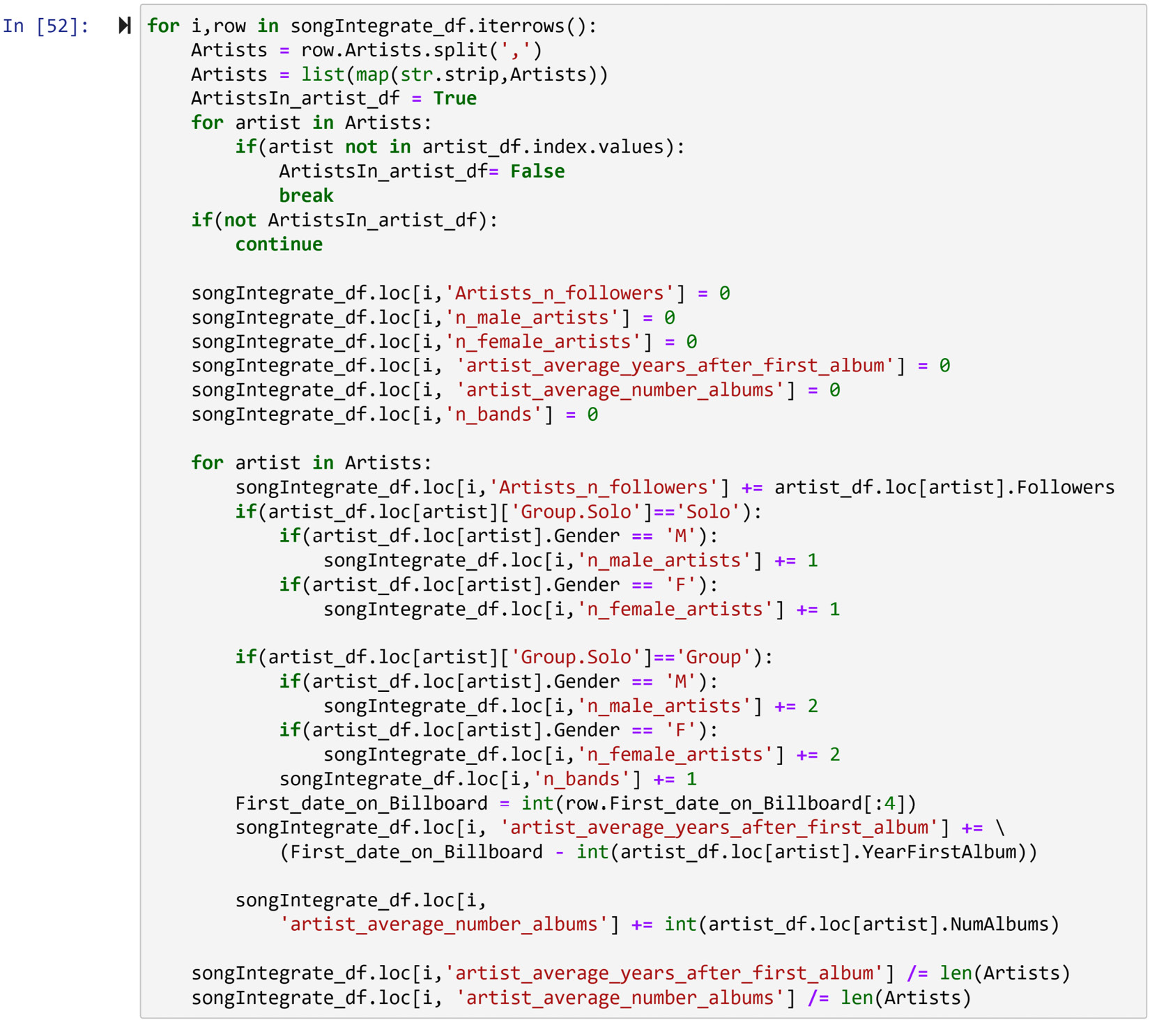
Figure 12.17 – Filling up the last six attributes of songIntegrate_df

You may have noticed that the code adds 2 to n_male_artists when the song's artist is a group and the gender is listed as male, while it adds 2 to n_female_artists when the song's artist is a group and the gender is listed as female. This includes the assumption that all the groups have only two artists. As we don't have other sources so that we can be more accurate about these situations, this is a reasonable assumption that lets us continue while avoiding the infliction of too much bias in the data. However, this assumption must be communicated if the results are going to be presented to any interested decision-maker.

After successfully running the preceding code, run songIntegrate_df.info() to investigate how many of the rows in songIntegrate_df were completed using the information from artist_df. You will see that 3,672 out of 4,045 songs were completed. While this is the major portion of songIntegrate_df, we still need to make sure that there are no missing values due to reasons connected to the songs being top songs or not. So, we will do a similar analysis to what we did for Figure 12.16. The following screenshot shows the result of the same analysis with the updated songIntegrate_df:

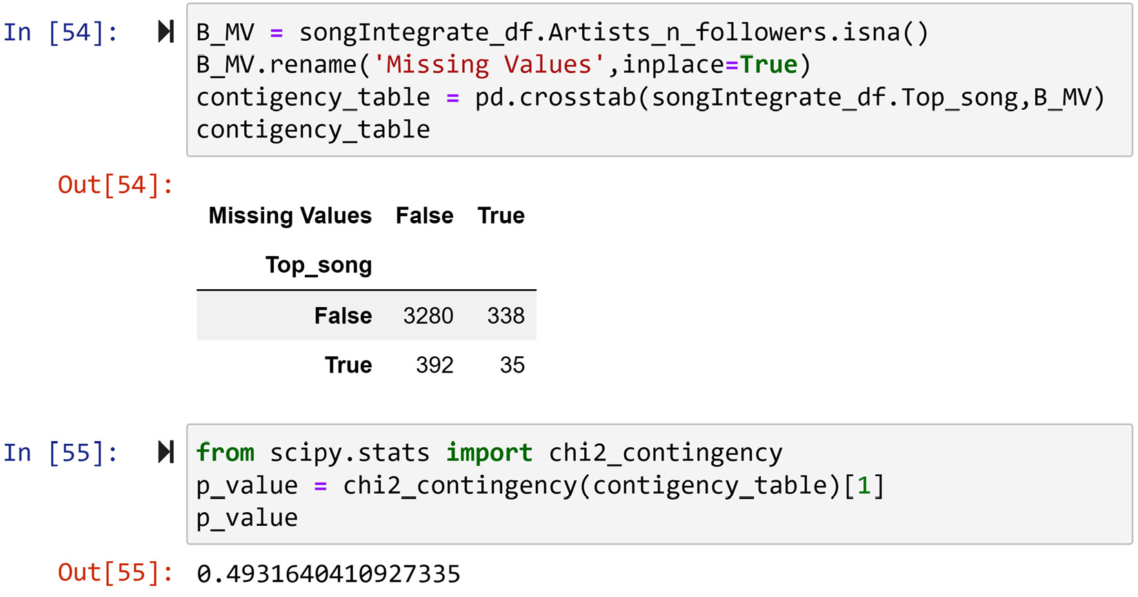
Figure 12.18 – The code and their output for studying if missing values in songIntegrate_df after integrating with artist_df are meaningfully connected to songIntegrate_df.Top_song

After studying the preceding screenshot, we can see that there is no meaningful pattern that points to the possible connection between a song being a top song and its tendency to have missing values at this juncture. So, we can comfortably remove the rows with missing values and proceed. The following line of code does the prescribed removal:

droping_indices = songIntegrate_df[B_MV].index.values

songIntegrate_df.drop(index = droping_indices, inplace=True)

The preceding code uses the .drop() function to delete the rows in songIntegrate_df that artist_df failed to fill. Note that the B_MV variable comes from the code in the preceding screenshot.

Congratulations – you have integrated these three data sources! This was due to your excellent understanding of data structures and your capability to see the definitions of data objects in each of these sources. Furthermore, you were able to envision a dataset that could house the information from all the sources and, at the same time, be useful for your analytic goals.

Before we proceed to the analysis, we need to tackle another challenge. Whenever we bring data together from different sources, we may have inadvertently created a case that we called data redundancy earlier (Challenge 6 – data redundancy). As we mentioned previously, data redundancy is where you repeat the same attribute but where you repeat the same information.

Checking for data redundancy

As we mentioned previously, this part deals with Challenge 6 – data redundancy. Even though we've never dealt with this challenge before in this book, we've seen many examples of investigating the relationships between attributes. If there are attributes in songIntegrate_df that have a strong relationship with each other, that can be our red flag for data redundancy. It's as simple as that!

So, let's get to it. First, we will use correlation analysis to investigate the relationship between the numerical attributes. Then, we will use box plots and t-tests to investigate the relationship between numerical attributes and categorical ones.

We would have investigated the relationships between categorical attributes as well if we didn't only have one categorical attribute. If you do have more than one categorical attribute, to evaluate data redundancy, you would need to use contingency tables and the chi-squared test of independence.

Checking for data redundancy among numerical attributes

As we mentioned previously, to evaluate the existence of data redundancy, we will use correlation analysis. If the correlation coefficient between two attributes is two high (we will use the rule thumb of 0.7), then this means that the information presented in the two attributes is too similar and there might be a case of data redundancy.

The following code uses the .corr() function to calculate the correlation between the numerical attributes that are explicitly listed in num_atts. The code also uses a Boolean mask (BM) to help our eyes find the correlation coefficient that is either greater than 0.7 or smaller than -0.7. Pay attention to the reason why the code had to include .astype(float): during the data integration process, some of the attributes may have been carried over as strings instead of numbers:

num_atts = ['Acousticness', 'Danceability', 'Duration', 'Energy', 'Instrumentalness', 'Liveness', 'Loudness', 'Mode', 'Speechiness', 'Tempo', 'TimeSignature', 'Valence', 'Artists_n_followers', 'n_male_artists', 'n_female_artists', 'n_bands', 'artist_average_years_after_first_album',   'artist_average_number_albums']

corr_Table = songIntegrate_df[num_atts].astype(float).corr()

BM = (corr_Table > 0.7) | (corr_Table<-0.7)

corr_Table[BM]

After running the preceding code successfully, a correlation matrix will appear that has NaN for most of the cells, but only for the ones that have had a correlation coefficient that's either greater than 0.7 or smaller than -0.7. You will notice that the only flagged correlation coefficient is between Energy and Loudness.

It makes sense that these two attributes have a relationship with one another. As these attributes come from the same source, we will put our confidence in the creators of these attributes that they do show different values and that around 30% of the information that is different between the two is worth keeping.

Here, we can conclude that there are no issues regarding data redundancy between the numerical attributes. Next, we will investigate whether the relationships between the categorical attributes and the numerical attributes are too strong.

Checking for data redundancy between numerical and categorical attributes

To evaluate if there is data redundancy, similar to what we did for the numerical attributes, we need to examine the relationship between the attributes. As the attributes are of different natures – that is, numerical and categorical – we need to use boxplots and t-tests.

The only categorical attribute that has been integrated and has analytic values at this point is the Explicit attribute. Why not the top_song attribute? The top song does have an analytic value for us – in fact, it is the hinge of our analysis – but it was not integrated from different sources. Instead, was calculated for our analysis. Once we get to the analysis part of this example, we will look at the relationship between this attribute and all the other ones. Why not Name or Artists? These are merely identifying columns. Why not First_date_on_Billboard? This was a temporary attribute to allow us to perform calculations where we needed information from more than one source of data. This attribute will be dropped before the analysis.

The following code creates the box plots that show the relationship between the numerical attribute and the categorical attribute; that is, Explicit. Furthermore, the code uses the ttest_ind() function from scipy.stats to run the t-test:

from scipy.stats import ttest_ind

for n_att in num_atts:

    sns.boxplot(data=songIntegrate_df, y=n_att,x='Explicit')

    plt.show()

    BM = songIntegrate_df.Explicit == True

    print(ttest_ind(songIntegrate_df[BM][n_att],                    songIntegrate_df[~BM][n_att]))

    print('-----------------divide-------------------')

After running the preceding code, per each numerical attribute, a box plot and the result of the t-test that evaluates the relationship between the Explicit attribute and the numerical attribute will appear. After studying the output, you will realize that the Explicit attribute has a relationship with all the numerical attributes except for Loudness, Mode, and Valence. As it is very unlikely that the Explicit attribute will contain any new information that has not already been included in the data, we will flag Explicit for possible data redundancy.

Note that we will not necessarily need to remove Explicit at the data preprocessing stage. How we will deal with data redundancy will depend on the analytic goals and the tools. For instance, if we intend to use a decision tree to see the multivariate patterns that lead to a song being a top song or not, then we won't need to do anything about the data redundancy. This is because the decision tree has a mechanism for selecting the features (attributes) that help with the success of the algorithm. On the other hand, if we are using K-means to group the songs, then we would need to remove Explicit as the information has already been introduced in the other attributes. If we include it twice, then it will create bias in our results.

The analysis

Finally, the data sources are appropriately integrated into songIntegrate_df and the dataset is ready for analysis. Our goal is to answer the question of what makes a song become a top song. There is more than one approach we can adopt here to answer this question, now that the data has been preprocessed. Here, we will use two of them. We will use data visualization to recognize the univariate patterns of top songs, and we will use a decision tree to extract the multi-variate patterns.

We will start with the data visualization process.

Before we start, there is no need to remove the Explicit attribute for any of the aforementioned analytic tools due to the attribute being flagged as redundant. As we mentioned previously, the decision tree has a smart mechanism for feature selection, so for data visualization, keeping Explicit will only mean one more simple visualization that does not interfere with the other visualizations.

The data visualization approach to finding patterns in top songs

To investigate what makes a song become a top song, we can investigate the relationship that all the other attributes in songIntegrate_df have with the Top_song attribute and see if any meaningful pattern emerges.

The following code creates a box plot for each of the numerical attributes in songIntegrate_df to investigate if the value of the numerical attribute changes in two populations: top songs and not top songs. The code also outputs the result of a t-test that answers the same question statistically. Furthermore, the code outputs the median of the two populations in case it is hard to recognize the minute comparisons between the values of the two populations in the box plots:

from scipy.stats import ttest_ind

for n_att in num_atts:

    sns.boxplot(data=songIntegrate_df, y=n_att,x='Top_song')

    plt.show()  

    BM = songIntegrate_df.Top_song == True

    print(ttest_ind(songIntegrate_df[BM][n_att], songIntegrate_    df[~BM][n_att]))

    dic = {'not Top Song Median': songIntegrate_df[~BM][n_att].    median(), 'Top Song Median': songIntegrate_df[BM][n_att].    median()}

    print(dic)

    print('-----------------divide-------------------')

Moreover, the following code outputs a contingency table that shows the relationship betweenn the two categorical attributes; that is, songIntegrate_df.Top_song and songIntegrate_df.Explicit. It also prints out the p-value of the chi-squared test of independence for these two categorical attributes:

from scipy.stats import chi2_contingency

contingency_table = pd.crosstab(songIntegrate_df.Top_song, songIntegrate_df.Explicit)

print(contingency_table)

print('p-value = {}'.format(chi2_contingency(contingency_table)[1]))

After studying the outputs of the two preceding pieces of code, we may come to the following conclusions:

• There is no evidence to reject the null hypothesis that the Top_song attribute does not have a relationship with the Duration, Energy, Instrumentalness, Liveness, Loudness, Mode, Speechiness, Explicit, and TimeSignature attributes. This means that the top songs cannot be predicted by looking at the values of these attributes.
• The top songs tend to have smaller values on the Acousticness, Tempo, n_male_artists, n_bands, artist_average_years_after_first_album, and artist_average_number_albums attributes.
• The songs that have greater values for the Danceability, Valence, Artists_n_followers, n_female_artists attributes tend to become top songs more often.

Of course, these patterns sound too general, and they should be; this is because they are univariate. Next, we will apply a decision tree to figure out the multivariate patterns, which may help us understand how a song becomes a top song.

The decision tree approach to finding multivariate patterns in top songs

As we discussed in Chapter 7, Classification, decision trees are famous for being transparent and being able to render useful multivariate patterns from the data. Here, we would like to use the decision tree algorithm to see the patterns that lead to a song raising to the top 10 list of the billboard.

The following code uses DecisionTreeClassifier from sklearn.tree to create a classification model that aims to find the relationships between the independent attributes and the dependent attribute; that is, Top_song. Once the model has been trained using this data, the code will use graphviz to visualize the trained decision tree. At the end of the code, the extracted graph will be saved in a file called TopSongDT.pdf. After successfully running this code, you should be able to find the file in the same folder where you have the Jupyter Notebook file.

Attention!

If you have never used graphviz on your computer before, you may have to install it first.

To install graphviz, all you need to do is run the following piece of code. After successfully running this code once, graphviz will be installed on your computer for good:

pip install graphviz

Before running the following code, note that the decision tree model that is used in the following code has already been tuned. In Chapter 7, Classification, we mentioned that tuning decision trees is very important. However, we have not covered how to do it in this book. The hyperparameters and their tuned values are criterion= 'entropy', max_depth= 10, min_samples_split= 30, and splitter= 'best':

from sklearn.tree import DecisionTreeClassifier, export_graphviz

import graphviz

y = songIntegrate_df.Top_song.replace({True:'Top Song',False:'Not Top Song'})

Xs = songIntegrate_df.drop(columns = ['Name','Artists','Top_song','First_date_on_Billboard'])

classTree = DecisionTreeClassifier(criterion= 'entropy', max_depth= 10, min_samples_split= 30, splitter= 'best')

classTree.fit(Xs, y)

dot_data = export_graphviz(classTree, out_file=None, feature_names=Xs.columns, class_names=['Not Top Song', 'Top Song'], filled=True, rounded=True, special_characters=True)  

graph = graphviz.Source(dot_data)

graph.render(filename='TopSongDT')

After successfully runing the preceding code, the TopSongDT.pdf file will be saved on your computer, which contains the visualized decision tree. This tree is shown in the following diagram. In this instance, this diagram has not be shared with you so that you can study it; as you can see, the decision tree is rather large and our space is very small. However, you can see that there are a lot of meanigful multi-variate patterns forming the data, which can help us predict the top songs:

Figure 12.19 – A decision tree that visualizes the multivariate patterns of the top songs

Open TopSongDT.pdf on your own and study it. For instance, you will see that the most important attribute for a distinction between top songs and non-top songs is Artists_n_followers. For another example, if the song does not have artists with high followings, the best shot the song has at becoming a top song is that the song is explicit, danceable, and from artists with less experience. There are many more useful patterns like this in the decision tree. Continue studying TopSongDT.pdf to find them.

Example summary

In this example, we performed many steps to get to a point where songIntegrate_df was in a state where we were able to perform analysis and find useful information. To jog our memory, these are the steps that we took:

1. Checked for duplicates in all three data sources
2. Designed the structure of the final and integrated dataset
3. Integrated the data sources in three steps
4. Checked for data redundancy
5. Performed analysis

Now, let's summarize the chapter.

Summary

Congratulations on your excellent progress in this chapter. First, we learned the difference between data fusion and data integration before becoming familiar with six common data integration challenges. Then, through three comprehensive examples, we used the programming and analytic tools that we've picked up throughout this book to face these data integration challenges and preprocess the data sources so that we were able to meet the analytic goals.

In the next chapter, we will focus on another data preprocessing concept that is crucial, especially for algorithmic data analytics due to the limitations of computational resources: data reduction.

Before you start your journey on data reduction, take some time and try out the following exercises to solidify your learning.

Exercise

1. In your own words, what is the difference between data fusion and data integration? Provides examples other than the ones given in this chapter.
2. Answer the following question about Challenge 4 – aggregation mismatch. Is this challenge a data fusion one, a data integration one, or both? Explain why.
3. How come Challenge 2 – unwise data collection is somehow both a data cleaning step and a data integration step? Do you think it is essential that we categorize an unwise data collection under data cleaning or data integration?
4. In Example 1 of this chapter, we used multi-level indexing using Date and Hour to overcome the index mismatched formatting challenge. For this exercise, repeat this example but this time, use single-level indexing using the Python DataTime object instead.
5. Recreate Figure 5.20 from Chapter 5, Data Visualization, but instead of using WH Report_preprocessed.csv, integrate the following three files yourself first: WH Report.csv, populations.csv, and Countries.csv. Hint: information about happiness indices come from WH Report.csv, information of the countries comes from Countries.csv, and population information comes from populations.csv.
6. In Chapter 6, Prediction, Exercise 2, we used ToyotaCorolla_preprocessed.csv to create a model that predicts the price of cars. In this exercise, we want to do the preprocessing ourselves. Use ToyotaCorolla.csv to answer the following questions:

   a) Are there any concerns regarding level I data cleaning? If so, address them if necessary.

   b) Are there any concerns regarding level II data cleaning? If so, address them if necessary.

   c) Are there any concerns regarding level III data cleaning? If so, address them if necessary.

   d) Are there any attributes in ToyotaCorolla.csv that can be considered redundant?

   e) Apply LinearRegression from sklearn.linear_model. Did you have to remove the redundant attributes? Why/why not?

   f) Apply MLPRegressor from sklearn.neural_network. Did you have to remove the redundant attributes? Why/why not?

7. We would like to use the Universities.csv file to put the universities into two meaningful clusters. However, the data source has many issues, including data cleaning levels I – III and data redundancy. Do the following:

   a) Deal with data cleaning issues.

   b) Deal with data redundancy issues.

   c) Use any column necessary except for State and Public (1)/ Private (2) to find the two meaningful clusters.

   d) Perform centroid analysis and name each cluster.

   e) Find out if the newly created categorical attribute cluster has a relationship with either of the two categorical attributes we intentionally did not use for clustering: State or Public (1)/ Private (2).

8. In this exercise, we will see an example of data fusion. The case study that we will use in this exercise was already introduced in the data fusion example for this chapter, so please go back and read it again before continuing with this exercise.

   In this example, we would like to integrate Yield.csv and Treatment.csv to see if the amount of water can impact the amount of yield.

   Do the following to make this happen:

   a) Use pd.read_csv() to read Yield.csv to yield_df, and read Treatment.csv into treatment_df.

   b) Draw a scatterplot of the points in treatment_df. Use the dimension of color to add the amount of water that has been dispensed from each point.

   c) Draw a scatterplot of the points in yield_df. Use the dimension of color to add the amount of harvest that has been collected from each point.

   d) Create a scatterplot that combines the visual in Steps b and c.

   e) From the scatterplots in the preceding steps, we can deduce that the water stations are equidistant from one another. Based on this realization, calculate the distance between the water points, and call it radius. We are going to use this variable in the following set of calculations.

   e) First, use the following code to create the calculateDistance() function:

   import math

   def calculateDistance(x1,y1,x2,y2):

       dist = math.sqrt((x2 - x1)**2 + (y2 - y1)**2)

       return dist

   Then, using the following code and the preceding function we just created, create the waterRecieved() function so that we can apply it to the function for the rows of treatment_df:

   def WaterReceived(r):

       w = 0

       for i, rr in treatment_df.iterrows():

           distance = calculateDistance(rr.longitude,         rr.latitude, r.longitude, r.latitude)

           if (distance< radius):

               w= w + rr.water * ((radius-distance)/radius)

       return w

   a) Apply waterRecieved() to the rows of yield_df and add the newly calculated value for each row to the water column.

   b) Study the newly updated yield_df. You just fused these two data sources. Go back and study these steps, especially the process of creating the waterRecieved() function. What are the assumptions that made this data fusion possible?

   c) Draw a scatterplot of the yield_df.harvest and yield_df.water attributes. Do we see any impact that yield_df.water has on yield_df.harvest?

   d) Use the correlation coefficient to confirm your observation from the previous step.