Chapter 7: Classification

As you learned how to go about predicting numerical values in the previous chapter, in this chapter, we will turn our attention to predicting categorical ones. Essentially, that is what classification is: predicting future categorical values. While prediction focuses on estimating what some numerical values will be in the future, classification predicts the occurrence or non-occurrence of events in the future. For instance, in this chapter, we will see how classification can predict whether an individual will default on their loan or not.

In this chapter, we will also discuss the procedural similarities and differences between prediction and classification and will cover two of the most famous classification algorithms: Decision Trees and K-Nearest Neighbors (KNN). While this chapter provides a fundamental understanding of classification algorithms and also shows how they are done using Python, this chapter cannot be looked at as a comprehensive reference for classification. Rather, you want to focus on the fundamental concepts so that you will be ready for your data preprocessing journey, which you will start in Chapter 9, Data Cleaning Level I – Cleaning Up the Table.

These are the main topics that this chapter will cover:

• Classification models
• KNN
• Decision Trees

Technical requirements

You will be able to find all of the code and the dataset that is used in this book in a GitHub repository exclusively created for this book. To find the repository, click on this link: https://github.com/PacktPublishing/Hands-On-Data-Preprocessing-in-Python. In this repository, you will find a folder titled Chapter07, from which you can download the code and the data for better learning.

Classification models

In the previous chapter, we covered predictive modeling. Classification is a type of predictive modeling; specifically, classification is a regression analysis where the dependent attribute or the target is categorical instead of numerical.

Even though classification is a subset of predictive modeling, it is the area of data mining that has received the most attention due to its usefulness. At the core of many machine learning (ML) solutions in the real world today is a classification algorithm. Despite its prevalent applications and complicated algorithms, the fundamental concepts of classification are simple.

Just as with prediction, for classification, we need to specify our independent attributes (predictors) and the dependent attribute (target). Once we are clear about these and we have a dataset that includes these attributes, we are set to employ classification algorithms.

Classification algorithms, just as with prediction algorithms, seek to find the relationship between independent attributes and the dependent attribute, so by knowing the values of the independent attributes of the new data object, we can guess the class of (classify) the new data object.

Let's now look at an example together so that these rather abstract concepts start making more sense to you.

Example of designing a classification model

When you apply for a cash loan these days, make no mistake that a classification algorithm is going to have a major role in deciding if you are going to get the loan or not. The classification models that are used in real cases tend to be very complex with many independent attributes. However, the two most important pieces of information these algorithms rely on are your income and credit score.

Here, we will present a simple version of these complex classifications. The classification design shown in the following diagram uses Income and Credit Score as independent attributes to classify if an applicant will default on an accepted loan or not. The Default? binary attribute is the dependent attribute of the classification design:

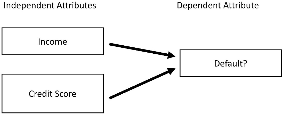
Figure 7.1 – Classification design of loan application problem

If you compare Figure 6.4 from the previous chapter with the preceding diagram, you might assert that there is no difference between prediction and classification; you would not be completely wrong. Prediction and classification are almost identical but for one simple distinction: a classification's dependent attribute is categorical, but a prediction's dependent attribute is numerical. That small distinction amounts to lots of algorithmic and analytic changes for these two data mining tasks.

Classification algorithms

There are many well-researched, -designed, and -developed classification algorithms. In fact, there are more classification algorithms than there are prediction algorithms. To name a few, we have KNN, Decision Trees, Multi-Layer Perceptron (MLP), Support Vector Machine (SVM), and Random Forest. Some of these algorithms are listed for both prediction and classification. For instance, MLP will always be listed for both; however, MLP is inherently designed for the prediction task, but it can be modified so that it can also successfully tackle classification. On the other hand, we have the Decision Trees algorithm, which is inherently designed for classification, but it can also be modified to address prediction.

In this chapter, we are going to be briefly introduced to two of these algorithms: KNN and Decision Trees.

KNN

KNN is one of the simplest classification algorithms, and almost everything you need to know about its mechanism is presented in its name. In simple terms, to classify a new data object, KNN finds the K-nearest neighbors to the new data object from the training dataset and uses the label of those data objects to assign the likely label of the new data object.

It might be the case that KNN is too simple, and because of that, you do not fully understand its mechanism. Let's continue our learning, using the following example.

Example of using KNN for classification

We are going to continue working on the loan application problem that was introduced earlier. After completing the classification design, we specified Income and Credit Score as independent attributes and Default? as the dependent attribute. The following screenshot shows a dataset that can support this classification design. The dataset is from the CustomerLoan.csv file:

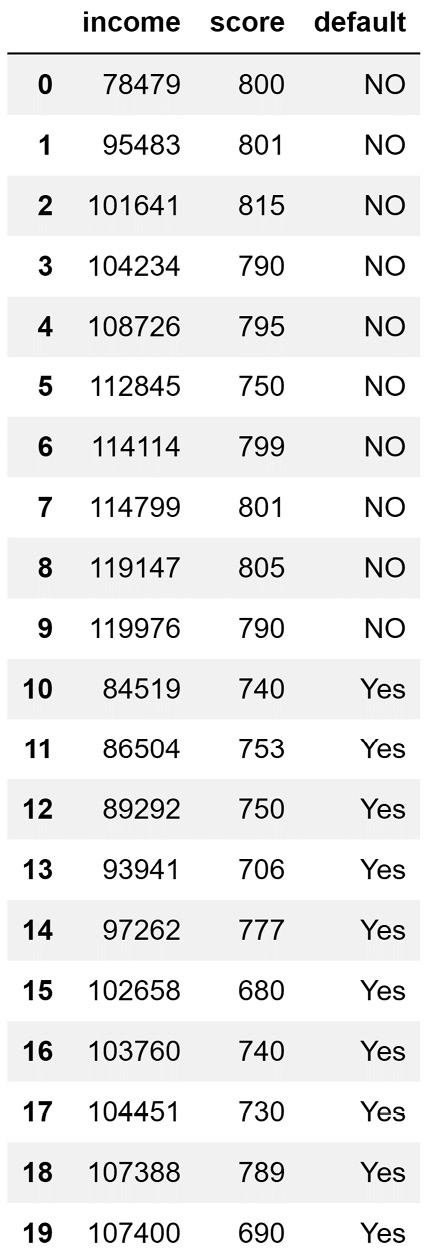
Figure 7.2 – CustomerLoan.csv file

Now, let's assume that we want to use the preceding data to classify whether a customer with a yearly income of US Dollars (USD) $98,487 and a credit score of 785 will default on a loan or not.

As this example only includes three dimensions, we can use visualizations to perform and understand the KNN algorithm. The following screenshot shows the classification problem we would like to solve at one glance:

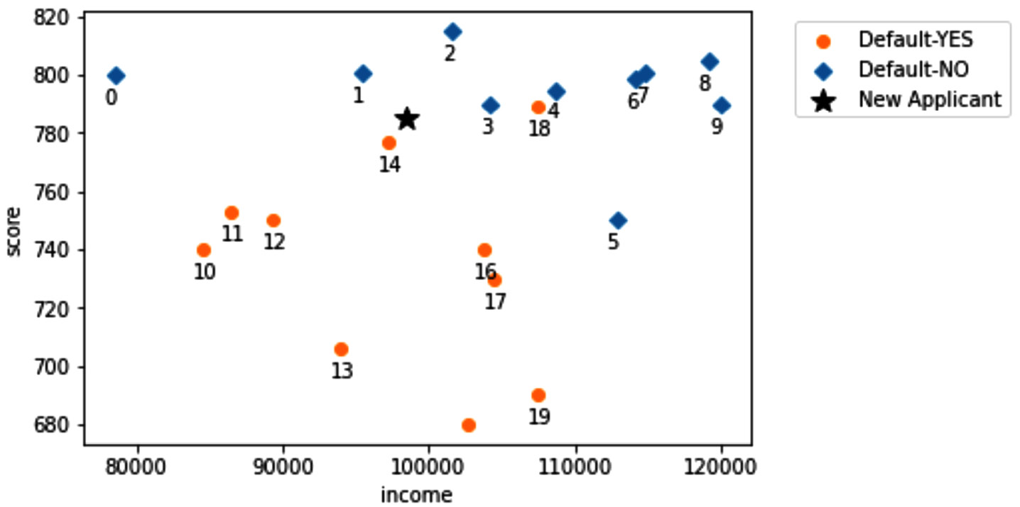
Figure 7.3 – Visualization of the loan application problem

The first step in performing KNN is to decide on K. Basically, we need to decide the number of nearest neighbors we would like to base our classification on. Let's assume we would like to use K=4.

Tuning KNN

Similar to many other data mining algorithms, to successfully use KNN for classification, you will need to tune the algorithm. Tuning KNN would mean finding the best number of K that would allow KNN to reach its best performance for every case study. In this book, we will not cover tuning as we are learning about algorithms, mainly to help us perform more successful data preprocessing.

So, when K=4, we can easily eyeball the preceding screenshot and see that the four nearest neighbors of the new applicant are data objects 1, 2, 3, and 14. As three out of four nearest data objects have a label of Default-NO, we will classify the new applicant as Default-NO. That is it—it's as simple as that.

While KNN is that simple in terms of its mechanism, creating a computer program that implements this algorithm is more difficult. Why is that? A few reasons are presented as follows:

• Here, we learned the mechanism of KNN, using an example that only had three dimensions. So, using a scatterplot and colors, we were able to display the problem and summarize all the data that we need to work with. Real-world problems will likely have more than just three dimensions.
• While we were able to eyeball the visual and detect the nearest neighbors, computers do not have the capability to just "see" which are the nearest neighbors. A computer program would need to calculate the distance between the new data object with all the data objects in the dataset so that it would find the K-nearest neighbors.
• What will happen if there is a tie? Let's say we have selected K=4, and two of the nearest neighbors are of one class and two others are from another.

  The great news for us is that we don't need to worry about any of these challenges because we can simply use a stable module that includes this algorithm. Let's import KNeighborsClassifier from the sklearn.neighbors module and apply it to our example here.

Before we can apply the algorithm, we need to take action about the following two matters:

1. First, if you have never used the sklearn module on Anaconda Navigator, you have to install it. Running the following code will install the module:

   conda install scikit-learn

2. Next, we will need to normalize our data. This is a data preprocessing concept, and we will cover it in depth when we get to it. However, let's briefly discuss its necessity here.

The reason that we need normalization of the data before applying KNN is that normally, the scale of the independent attributes are different from one another, and if the data is not normalized, the attribute with the larger scale will end up being more important in the distant calculation of the KNN algorithm, effectively canceling the role of other independent attributes. In this example, income ranges from 78,479 to 119,976, while score (for credit score) ranges from 680 to 815. If we were to calculate the distance between the data objects using these scales, all that would matter is income and not credit score.

So, to avoid letting the scale of the attributes meddle with the mechanism of the algorithm, we will normalize the data before using KNN. When an attribute is normalized, its values are transformed so that the updated attribute ranges from 0 to 1 without influencing the attribute's relative differentiation between the data objects.

The following code reads the CustomerLoan.csv file into the applicant_df DataFrame and creates two new columns in applicant_df that are the normalization transformation of the two columns in the original data:

applicant_df = pd.read_csv('CustomerLoan.csv')

applicant_df['income_Normalized'] = (applicant_df.income - applicant_df.income.min())/(applicant_df.income.max() - applicant_df.income.min())

applicant_df['score_Normalized'] = (applicant_df.score - applicant_df.score.min())/(applicant_df.score.max() - applicant_df.score.min())

The preceding code has created two new columns by using the following formula:

The preceding code has used the formula to transform the income column to income_Normalized, and score to score_Normalized. The following screenshot shows the result of this data transformation:

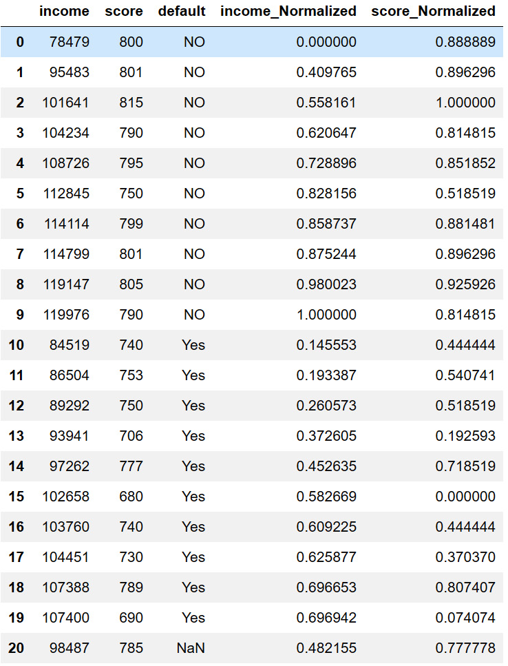
Figure 7.4 – Transformed applicant_df DataFrame

Take a moment to study the preceding screenshot; specifically, see the relationship between the columns and their normalized version. You will notice that the relevant distance and order between the values under the original attribute and its normalized version do not change. To see this, find the minimum and maximum under both the original attribute and its normalized version, and study those.

Pay attention to the fact that the last row of the data in the preceding screenshot is the new applicant that we would like to classify.

Now that the data is ready, we can apply the KneighborsClassifier module from sklearn.neighbors to do this. You can carry this out in four steps, as follows:

1. First, the KneighborsClassifier module needs to be imported. The following code does the import:

   from sklearn.neighbors import KNeighborsClassifier

2. Next, we need to specify our independent attributes and the dependent attribute. The following code keeps the independent attributes in Xs and the dependent attribute in y.

   Pay attention to the fact that we are dropping the last row of the data, as this is the row of the data we want to perform the prediction for. The .drop(index=[20]) part will take care of this dropping:

   predictors = ['income_Normalized','score_Normalized']

   target = 'default'

   Xs = applicant_df[predictors].drop(index=[20])

   y= applicant_df[target].drop(index=[20])

3. Next, we will create a KNN model and then fit the data into it. The following code shows how this is done:

   knn = KNeighborsClassifier(n_neighbors=4)

   knn.fit(Xs, y)

4. Now, knn is ready to classify the new data objects. The following code shows how we can separate the last row of the dataset and make a prediction for it using knn:

   newApplicant = pd.DataFrame({'income_Normalized': applicant_df.iloc[20].income_Normalized,'score_Normalized': applicant_df.iloc[20].score_Normalized},index = [20])

   predict_y = knn.predict(newApplicant)

   print(predict_y)

   If you put all the preceding four code snippets together, you will get the following output, which also reports the prediction for newApplicant:

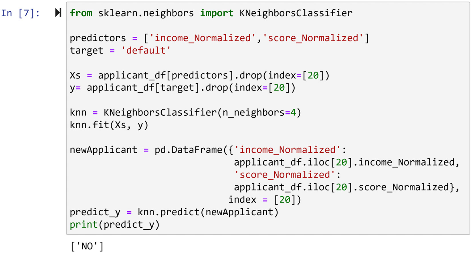
Figure 7.5 – Classification using sklearn.neighbors

The output in the preceding screenshot, which is the class for newApplicant, confirms the conclusion we had already decided that KNN should arrive at.

So far in this chapter, you have learned about classification analysis, and you have also learned how the KNN algorithm works and how to get KneighborsClassifier from the sklearn.neighbors module to apply KNN to a dataset. Next, you will be introduced to another classification algorithm: Decision Trees.

Decision Trees

While you can use the Decision Trees algorithm for classification, just like KNN, it goes about the task of classification very differently. While KNN finds the most similar data objects for classification, Decision Trees first summarizes the data using a tree-like structure and then uses the structure to perform the classification.

Let's learn about Decision Trees using an example.

Example of using Decision Trees for classification

We will use DecisionTreeClassifier from sklearn.tree to apply the Decision Trees algorithm to applicant_df. The code needed to use Decision Trees is almost identical to that of KNN. Let's see the code first, and then I will draw your attention to their similarities and differences. Here it is:

from sklearn.tree import DecisionTreeClassifier

predictors = ['income','score']

target = 'default'

Xs = applicant_df[predictors].drop(index=[20])

y= applicant_df[target].drop(index=[20])

classTree = DecisionTreeClassifier()

classTree.fit(Xs, y)

predict_y = classTree.predict(newApplicant)

print(predict_y)

There are two differences between the preceding code and the KNN code. Here, we list these differences:

• First, the decision tree, due to the way it works, does not need the data to be normalized, so that is why the predictors = ['income','score'] line of code uses the original attributes. We used the normalized version for KNN.
• Second, and obviously, we have used DecisionTreeClassifier() instead of KneighborsClassifier(). We also named our classification model classTree here, as opposed to knn, which we used for KNN.

  Pay Attention!

  As you probably have noticed, the code to use any predictive model (prediction and classification) in Python is very similar. Here are the steps we take for every single one of the models. First, we import the module that has the algorithm we would like to use. Next, we separate the data into independent and dependent attributes. After that, we create a model using the module we imported. Then, we use the .fit() function of the model we created to fit the data into the model. Lastly, we use the .predict() function to predict the dependent attribute for the new data objects.

If you successfully run the preceding code, you will see that the decision tree, unlike KNN, classifies newApplicant as YES. Let's look at the tree-like structure that DecisionTreeClassifier() created to come to this conclusion. To do this, we will use the plot_tree() function from the sklearn.tree module. Try running the following code to draw the tree-like structure:

from sklearn.tree import plot_tree

plot_tree(classTree,          feature_names=predictors,          class_names=y.unique(),          filled=True,          impurity=False)

The preceding code will output the following:

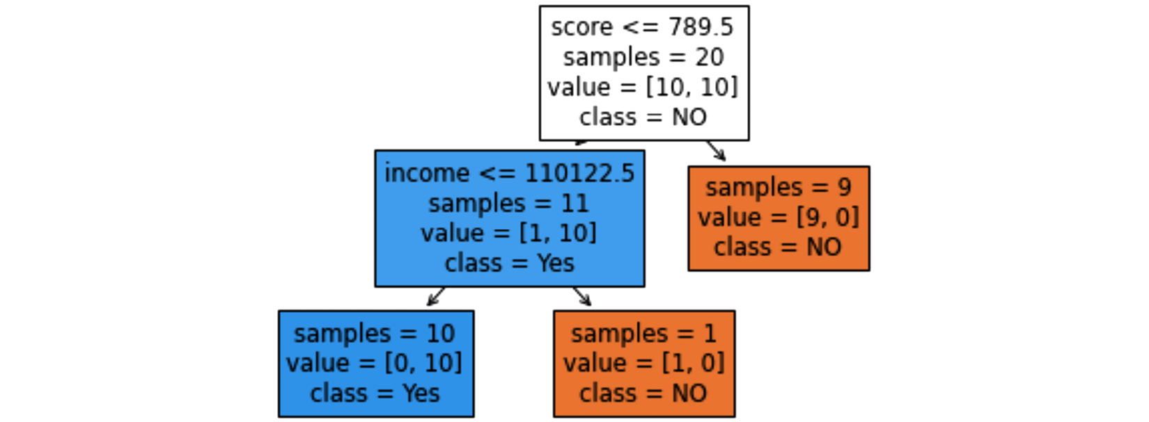
Figure 7.6 – Classification using sklearn.neighbors

The output in the preceding screenshot will intuitively tell you why Decision Trees arrived at a different conclusion from that of KNN. Starting from the top node, the dataset is separated into two groups: data objects whose scores are greater than 789.5 and data objects whose scores are lower than the cutoff value. All of the data objects with scores higher than 789.5 are labeled NO-default; therefore, the decision tree has come to the conclusion that if an applicant's score is higher than 789.5, they should be classified as NO.

Since the score of newApplicant is 785, this rule does not apply to this data object. To find the class of the data object based on this tree-like structure. we need to go deeper. From the tree-like structure, we see that the data object that has scores lower than 789.5 and an income lower than 110,122.5 has defaulted on the loan. So, again, Decision Trees has reached the rule that when applicant scores are lower than 789.5 and 110,122.5, they should be classified as YES. As the score and income of newApplicant are both lower than these cutoff values, the decision tree has concluded YES for it.

Tuning Decision Trees

Just as with KNN, Decision Trees also needs tuning to reach its fullest potential. In fact, Decision Trees requires even more tuning than what KNN needs, as Decision Trees has more hyperparameters that could be adjusted. However, for the same reasons mentioned for KNN, we will not cover the how-to of the tunings in this book.

The way Decision Trees works is also simple—Decision Trees splits the dataset into two segments again and again, at different stages, using one of the independent attributes until all segments of the data are pure. Purity means that all of the data in the segment is of the same class.

Before making our way to the end of this chapter, let's take a moment to discuss why the two algorithms have reached a different conclusion. First, we need to understand that when two distinct algorithms arrive at different conclusions about the same data object, this is a sign that classification of that data object is difficult, meaning that there are different patterns in the data that show the data object could be either of the classes. Second, as these algorithms have various ways of pattern recognition and decision-making, the algorithms that conclude differently may have prioritized the patterns in dissimilar ways.

Summary

Congratulations on your excellent progress in this chapter! Together, we learned the fundamental concepts and techniques of classification analysis. Specifically, we understood the distinction between classification and prediction, and we also learned about two famous classification algorithms and used them on a sample dataset to understand them even deeper.

In the next chapter, we will cover another important analytics task: clustering analysis. We will use the famous K-Means algorithm to learn more about clustering and also run a few experiments.

Before moving forward and starting your journey to learn about clustering, spend some time on the following exercises and solidify your learning.

Exercises

1. The chapter asserts that before using KNN, you will need to have your independent attributes normalized. This is certainly true, but how come we were able to get away with no normalization when we performed KNN using visualization? (See Figure 7.3.)
2. We did not normalize the data when applying Decision Trees to the loan application problem. For practice and a deeper understanding, apply Decision Trees to the normalized data, and answer the following questions:

   a) Did the conclusion of Decision Trees change? Why do you think that is? Use the mechanism of the algorithm to explain.

   b) Did the Decision Trees tree-like structure change? In what ways? Did the change make a meaningful difference in the way that the tree-like structure could be used?

3. For this exercise, we are going to use the Customer Churn.csv dataset. This dataset is randomly collected from an Iranian telecom company's database over a period of 12 months. A total of 3,150 rows of data, each representing a customer, bear information for 9 columns. The attributes that are in this dataset are listed here:

   Call Failures: Number of call failures

   Complaints: Binary (0: No complaint; 1: complaint)

   Subscription Length: Total months of subscription

   Seconds of Use: Total seconds of calls

   Frequency of Use: Total number of calls

   Frequency of SMS: Total number of text messages

   Distinct Called Numbers: Total number of distinct phone calls

   Status: Binary (1: active; 0: non-active)

   Churn: Binary (1: churn; 0: non-churn)—class label

   All of the attributes except for attribute churn are the aggregated data of the first 9 months. The churn labels are the state of the customers at the end of 12 months. 3 months is the designated planning gap.

   Using the preceding data, we would like to use this dataset to predict if the following customer will churn in 3 months:

   Call Failures: 8; Complaints: 1; Subscription Length: 40; Seconds of Use: 4,472; Frequency of Use: 70; Frequency of SMS: 100; Distinct Called Numbers: 25; Status: 1.

   To do this, perform the following steps:

   a) Read the data into the pandas customer_df DataFrame.

   b) Use the skills you picked up in Chapter 5, Data Visualization, to come up with data visualizations that show the relationship between the churn attribute and the rest of the attributes.

   c) Use the visuals in Step 2 to describe the relationship each of the attributes has with the attribute Churn.

   d) Perform KNN to predict if the aforementioned customer will be churned using all of the attributes that had a meaningful relationship with churn. Do you need to normalize the data first? Use K=5.

   e) Repeat Step 4, but this time use K=10. Are the conclusions different?

   f) Now, use the Decision Trees algorithm for classification. Do you need to normalize the data? Use max_depth=4. Is the conclusion of the Decision Trees algorithm different from that of the KNN algorithm?

   max_depth is a hyperparameter of the Decision Trees algorithm that controls how deep the learning can be. The number that is assigned is the maximum number of splits from the root of the tree.

   g) Draw the tree-like structure of the decision tree and explain how the decision tree came to the conclusion it did.