Chapter 9: Data Cleaning Level I – Cleaning Up the Table

We are finally here! After making sure that we have the required technical skills (part 1 of this book) and analytics skills (part 2 of this book), we can start discussing effective data preprocessing. We will start this journey by looking at data cleaning. This chapter divides data cleaning into three levels: levels I, II, and III. As you move up these levels, learning about the concept of data cleaning will become deeper and more complex. We will talk about what they are, how they are different, and what types of situations require us to perform each level of data cleaning. Furthermore, for each level of data cleaning, we will see examples of data sources that will require different levels of data cleaning.

In this chapter, we will focus on data cleaning level I – cleaning up the table. The next two chapters are also dedicated to data cleaning but at levels II and III.

In this chapter, we're going to cover the following main topics:

• The levels, tools, and purposes of data cleaning – a roadmap to Chapter 9, Data Cleaning Level I – Cleaning Up the Table, Chapter 10, Data Cleaning Level II – Unpacking, Restructuring, and Reformulating the Table, and Chapter 11, Data Cleaning Level III – Missing Values, Outliers, and Errors
• Data cleaning level I – cleaning up the table

Technical requirements

You can find all of the code and the dataset for this book in this book's GitHub repository. To find the repository, go to https://github.com/PacktPublishing/Hands-On-Data-Preprocessing-in-Python. You can find Chapter09 in this repository and download the code and the data to aid with your learning.

The levels, tools, and purposes of data cleaning – a roadmap to chapters 9, 10, and 11

One of the most exciting moments in any data analytics project is when you have one dataset that you believe contains all the data you need to effectively meet the goals of the project. This moment comes normally in one of the following situations:

• You are done collecting data for the analysis you have in mind.
• You have done extensive data integration from different data sources. Data integration is a very important skillset and we will cover it in Chapter 12, Data Fusion and Data Integration.
• The dataset is just shared with you and it contains everything that you need.

Regardless of how you got your hands on the dataset, this is an exciting moment. But beware that more often than not, you still have many steps to take before you can analyze the data. First, you need to clean the dataset.

To learn about and perform data cleaning, we need to fully understand the following three aspects:

• Purpose of data analytics: Why are we cleaning the dataset? In other words, how are we going to use the dataset once it has been cleaned?
• Tools for data analytics: What will be used to perform data analytics? Python (Matplotlib/sklearn)? Excel? MATLAB? Tableau?
• Levels of data cleaning: What aspects of the dataset need cleaning? Is our cleaning at the surface level, in that we are only cleaning up the name of the columns, or is our cleaning deeper, in that we are making sure that the recorded values are correct?

In the next three subsections, we will look at each of these aspects in more detail.

Purpose of data analytics

While it might sound like data cleaning can be done separately without us paying too much attention to the purpose of the analysis, in this chapter, we will see that more often than not, this is not the case. In other words, you will need to know what analytics you will be performing on the dataset when you are cleaning your data. Not only that, but you also need to know exactly how the analytics and perhaps the algorithms that you have in mind will be using and manipulating the data.

So far in this book, we have learned about four different data analytic goals: data visualization, prediction, classification, and clustering. We learned about these analytics goals and how data is manipulated to meet them. We needed a more profound level of understanding and appreciation for these goals so that they can support our data cleaning. By knowing how the data will be used after we have cleaned it, we are in a position to make better decisions regarding how the data should be cleaned. In this chapter, we will see that our deeper understanding of the analytic goals will guide us to perform more effective data cleaning.

Tools for data analytics

The software tools you intend to use will also have a major role in how you will go about data cleaning. For instance, if you intend to use MATLAB to perform clustering analysis and you've completed data cleaning in Python and have the completed data in Pandas DataFrame format, you will need to transform the data into a structure that MATLAB can read. Perhaps you could use .to_csv() to save the DataFrame as a .csv file and open the file in MATLAB since .csv files are compatible with almost any software.

Levels of data cleaning

The data cleaning process has both high-level goals and many nitty-gritty details. Not only that but what needs to be done for data cleaning from one project to another can be completely different. So, it is impossible to give clear-cut, step-by-step instructions on how you should go about data cleaning. However, we can loosely place the data cleaning procedure at three levels, as follows:

1. Level I: Clean up the table.
2. Level II: Unpack, restructure, and reformulate the table.
3. Level III: Evaluate and correct the values.

In this chapter and the next two, we will learn about various data cleaning situations that fall under one of the preceding levels. While each of these levels will have a specific section in this book, we will briefly go over what they are and how they differ from one another here.

Level I– cleaning up the table

This level of cleaning is all about how the table looks. A level I cleaned dataset has three characteristics: it is in a standard data structure, it has codable and intuitive column titles, and each row has a unique identifier.

Level II– restructuring and reformulating the table

This level of cleaning has to do with the type of data structure and format you need your dataset to be in so that the analytics you have in mind can be done. Most of the time, the tools you use for analytics dictate the structure and the format of the data. For instance, if you need to create multiple box plots using plt.boxplot(), you need to separate the data for each box plot. For instance, see the Comparing populations using box plots example in the Comparing populations section of Chapter 5, Data Visualization, where we restructured the data before using the function to draw multiple box plots.

Level III– evaluating and correcting the values

This level of cleaning is about the correctness and existence of the recorded values in the dataset. At this level of cleaning, you want to make certain that the recorded values are correct and are presented in a way that best supports the analytics goals. This level of data cleaning is the most technical and theoretical part of the data cleaning process. Not only do we need to know how the tools we will be using need the data to be, but we also need to understand how the data should be corrected, combined, or removed, as informed by the goals of the analytics process. Dealing with missing values and handling outliers are also major parts of this level of data cleaning.

So far, we have looked at the three most important dimensions of data cleaning: the purpose of data analytics, the tools for data analytics, and the three data cleaning levels. Next, we will understand the roles these three dimensions – analytics purposes, analytic tools, and the levels of data cleaning – play when it comes to effective data cleaning.

Mapping the purposes and tools of analytics to the levels of data cleaning

The following diagram shows the map of these three dimensions. Having a dataset that has been cleaned at level I is the very first step, and taking the time to make sure this level of data cleaning has been performed will make the next data cleaning levels and the data analytics process easier. While we can perform data cleaning level I without knowing the analytics we have for the dataset, it would be unwise to do any level II or level III data cleaning without knowing the software tools or the analytics you intend to employ. The following diagram shows that level II data cleaning needs to be done while you're informed about the tools and the analytic goals, while level III data cleaning needs to be executed once you know about the data analytics goals:

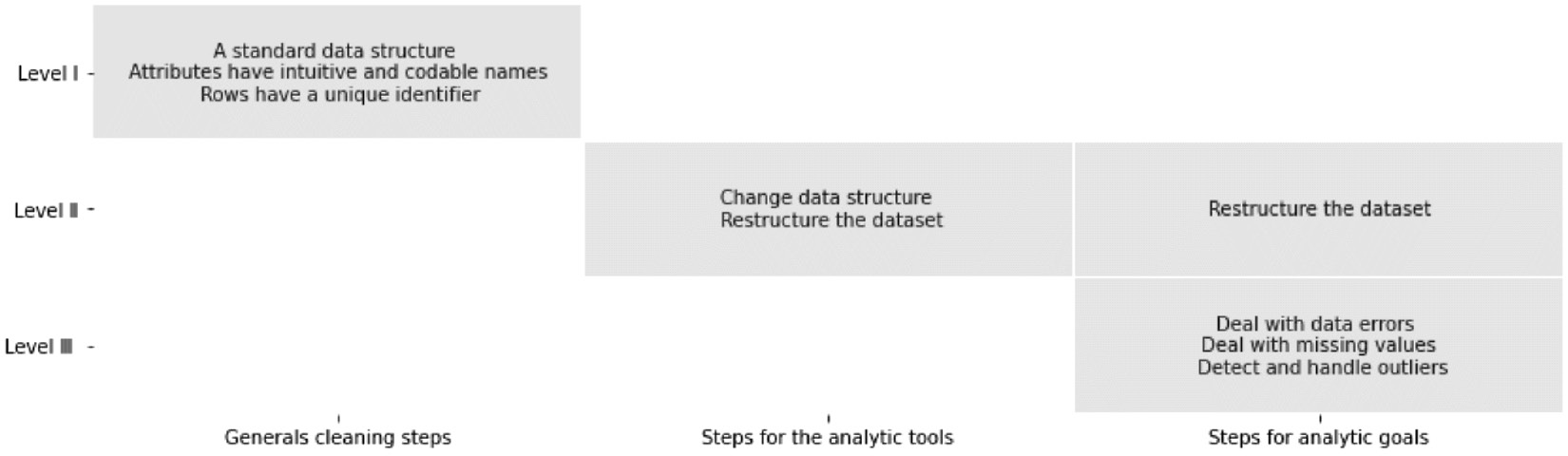
Figure 9.1 – Relevant amount of general and specific steps for three different levels of data cleaning

In the remainder of this chapter, we will cover data cleaning level I in more detail by providing data cleaning examples that tend to occur frequently. In the next few chapters, we will do the same thing for data cleaning levels II and III.

Data cleaning level I – cleaning up the table

Data cleaning level I has the least deep data preprocessing steps. Most of the time, you can get away with not having your data cleaned at level I. However, having a dataset that is level I cleaned would be very rewarding as it would make the rest of the data cleaning process and data analytics much easier.

We will consider a level I dataset clean where the dataset has the following characteristics:

• It is in a standard and preferred data structure.
• It has codable and intuitive column titles.
• Each row has a unique identifier.

The following three examples feature at least one or a combination of the preceding characteristics for ease of learning.

Example 1 – unwise data collection

From time to time, you might come across sources of data that are not collected and recorded in the best possible way. These situations occur when the data collection process has been done by someone or a group of people who don't have the appropriate skills regarding database management. Regardless of why this situation might have occurred, you are given access to a data source that requires significant preprocessing before it can be put in one standard data structure.

For instance, imagine that you have been hired by an election campaign to use the power of data to help move the needle. Omid was hired just before you, and he knows a lot about the political aspects of the election but not much about data and data analytics. You have been assigned to join Omid and help process what he has been tasked with. In your first meeting, you realize that the task is to analyze the speeches that have been made by the 45th President of the United States, Donald Trump. To bring you up to speed, he smiles and tells you that he has completed the data collection process and that all that needs to be done is the analysis now; he shows you a folder on his computer that contains text files (.txt) for every one of Donald Trump's speeches made in 2019 and 2020. The following screenshot shows this folder on Omid's computer:

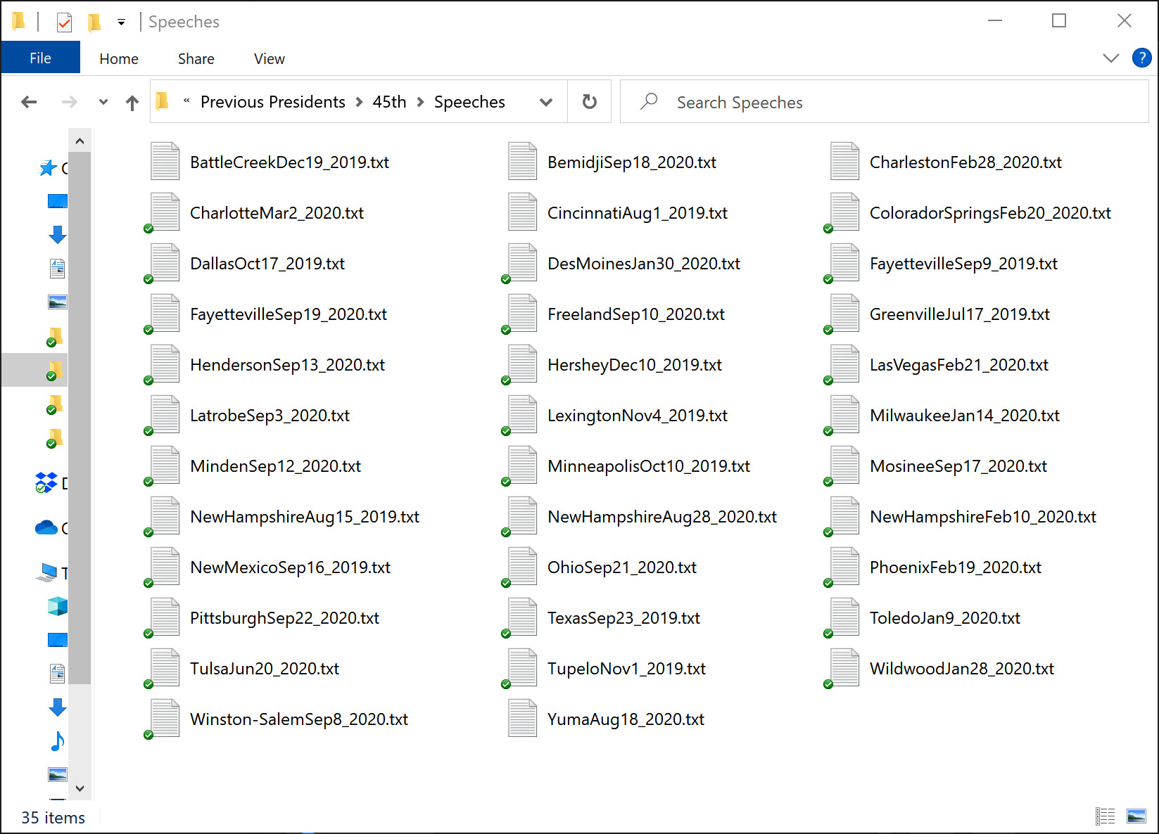
Figure 9.2 – Example of unwise data collection

After viewing the folder, you instantly realize that data preprocessing must be done before any analytics can be considered. In the interest of building a good working relationship with Omid, you don't tell him directly that a huge data preprocessing task needs to be done; instead, you comment on the aspects of his data collection that are great and can be used as a cornerstone for data preprocessing. You mention that it is great that the naming of these files follows a predictable order. The order is that city names come first, comes the name of the month as three letters, then the day as one or two digits, and finally the year as four digits.

As you are well-versed with Pandas DataFrame, you suggest that the data should be processed into a DataFrame and Omid, eager to learn, accepts.

You can perform the following steps to process the data into a DataFrame:

1. First, we need to access the filenames so that we can use them to open and read each file. Pay attention: we can type the names of the files ourselves as there are only 35 of them. However, we must do this using programing as we are trying to learn scalable skills; imagine that we have one million files instead of 35. The following code shows how using the listdir() function from the os module can do that for us very easily:

   from os import listdir

   FileNames = listdir('Speeches')

   print(FileNames)

2. Next, we need to create a placeholder for our data. In this step, we need to imagine what our dataset would look like after this data cleaning process has been completed. We want to have a DataFrame that contains the names of each file and its content. The following code uses the pandas module to create this placeholder:

   import pandas as pd

   speech_df = pd.DataFrame(index=range(len(FileNames)), columns=['File Name','The Content'])

   print(speech_df)

3. Lastly, we need to open each file and insert its content into speech_df, which we created in the previous step. The following code loops through the elements of FineNames. As each element is the name of one of the files that can be used to open and read the file, we can use the open() and .readlines() functions here:

   for i,f_name in enumerate(FileNames):

       f = open('Speeches/' + f_name, "r", encoding='utf-8')

       f_content = f.readlines()

       f.close()

       speech_df.at[i,'File Name'] = f_name

       speech_df.at[i,'The Content'] = f_content[0]

Once you have completed these three steps, run Print(speech_df) and study it before moving on. Here, you can see that speech_df has two of the three characteristics of level I cleaned data. The dataset has the first characteristics as it is now one standard data structure, which is also your preferred one.

The dataset, after being processed into speech_df, also has the third characteristic as each row has a unique index. You can run speech_df.index to investigate this. You might be pleasantly surprised that we didn't do anything to acquire this cleaning characteristic. This is automatically done for us by Pandas.

However, we could have done better regarding the second characteristic. The File Name and The Content column names are intuitive enough, but they are not as codable as they can be. We can access them using the df['ColumnName'] method but not df.ColumnName, as shown here:

1. First, run speech_df['File Name'] and speech_df['The Content']; you will see that you can easily access each column using this method.
2. Second, run speech_df.File Name and speech_df.The Content; you will get errors. Why? To jog your memory, please go back to Chapter 1, Reviewing the Core Modules of NumPy and Pandas, find the DataFrame access columns section, and study the error shown in Figure 1.16. The cause of the error is very similar here.

So, to make the column titles codable when using a Pandas DataFrame, we only have to follow a few guidelines, as follows:

• Try to shorten the column's titles as much as possible without them becoming unintuitive. For instance, The Content can simply be Content.
• Avoid using spaces and possible programming operators such as -, +, =, %, and & in the names of the columns. If you have to have more than one word as the column's name, either use camel case naming (FileName) or use an underscore (File_Name).

You may have noticed in the second to last piece of code that I could have used more codable column titles; I could have used columns=['FileName','Content'] instead of columns=['File Name','The Content']. You are right. I should have done this there; I only did this so I was able to make this point afterward. So, go ahead and improve the code before moving on. Alternatively, you can use the following code to change the column names to their codable versions:

speech_df.columns = ['FileName','Content']

Now that we have completed this example, let's review the characteristics of Level I data cleaning that the sources of data in this example needed. This source of data needed all three characteristics of Level I data cleaning to be improved. We had to take action explicitly to make sure that the data is in standard data structure and also has intuitive and codable column names. Also, the tool we used, Pandas, automatically gave each row a unique identifier.

Example 2 – reindexing (multi-level indexing)

In this example, we want to perform Level 1 data Cleaning on TempData.csv. The following screenshot shows how to use Pandas to read the data into a DataFrame:

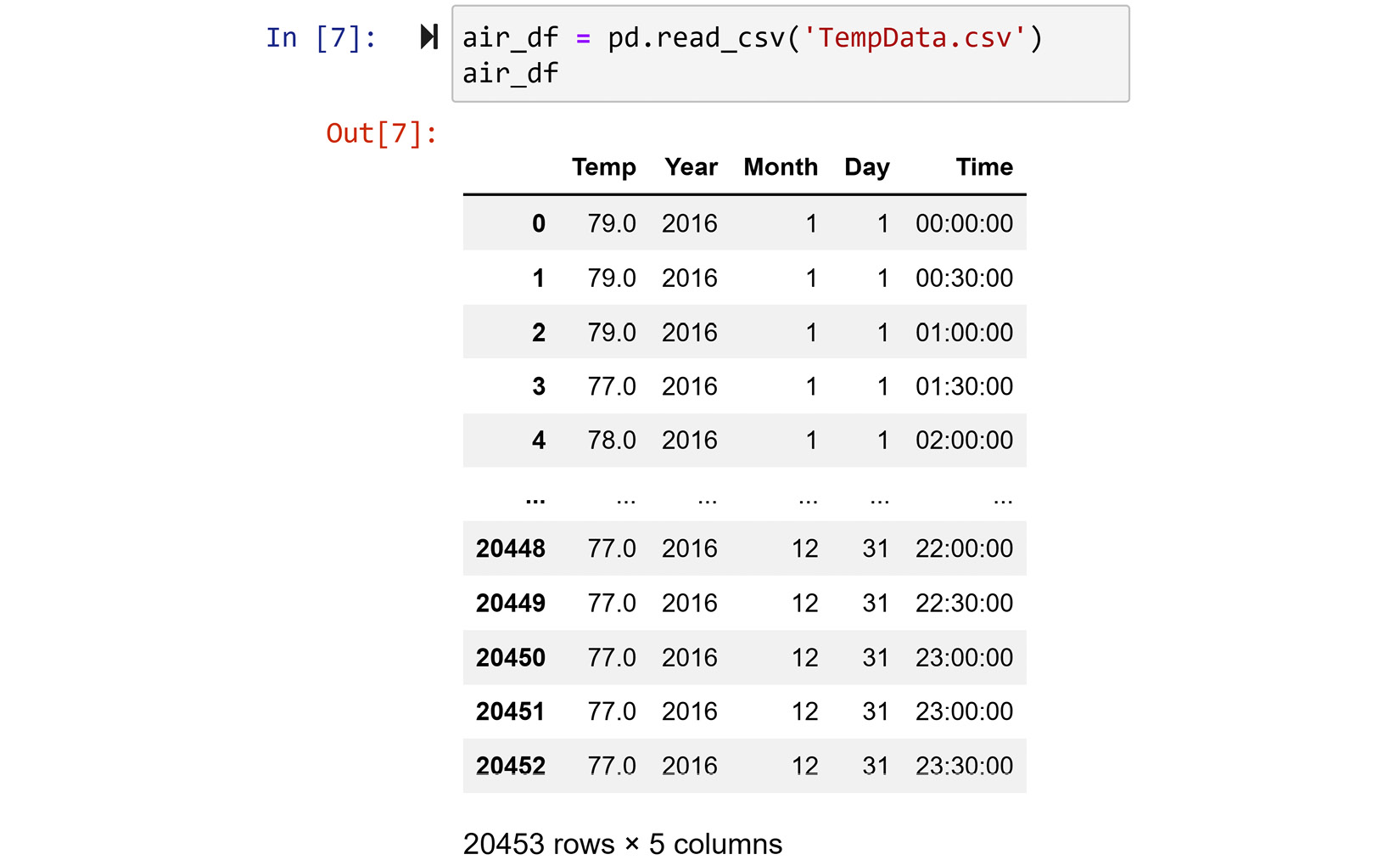
Figure 9.3 – Reading TempData.CSV into a Pandas DataFrame

Our first evaluation of the dataset reveals that the data is in one standard data structure, the column titles are intuitive and codable, and each row has a unique identifier. However, upon looking at this more closely, the default indices assigned by Pandas are unique but not helpful for identifying the rows. The Year, Month, Day, and Time columns would be better off as the indexes of the rows. So, in this example, we would like to reindex the DataFrame using more than one column. We will use Pandas's special capability known as multi-level indexing. We covered this in the Pandas multi-level indexing section Chapter 1, Reviewing the Core Modules of NumPy and Pandas.

This can be done easily by using the .set_index() function of a Pandas DataFrame. However, before we do that, let's remove the Year column as its value is only 2016. To check this, run air_df.Year.unique(). In the following line of code, so that we don't lose the information stating that this dataset is for 2016, we will change the DataFrame's name to air2016_df:

air2016_df = air_df.drop(columns=['Year'])

Now that the unnecessary column has been removed, we can use the .set_index() function to reindex the DataFrame:

air2016_df.set_index(['Month','Day','Time'],inplace=True)

If you print air2016_df after running the preceding code, you will get the DataFrame with a multi-level index, as shown in the following screenshot:

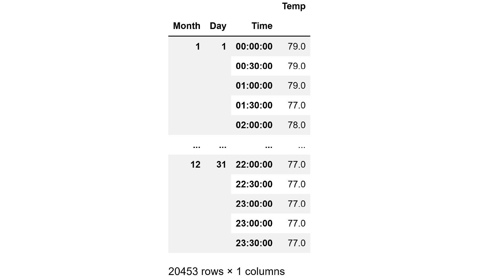
Figure 9.4 – air2016_df with a multi-level index

Our achievement here is that not only does each row have a unique index but the indices can be used to meaningfully identify each row. For instance, you can run air2016_df.loc[2,24,'00:30:00'] to get the temperature value of February 24 at 30 minutes after midnight.

In this example, we focused on the third characteristic of level I data cleaning: each row has a unique identifier. In the following example, we will focus on the second characteristic: having a codable and intuitive column name.

Example 3 – intuitive but long column titles

In this example, we will be using OSMI Mental Health in Tech Survey 2019.csv from https://osmihelp.org/research. The following screenshot shows the code that reads the dataset into response_df, and then uses the .head() function to show the first row of the data:

Figure 9.5 – Reading data into response_df and showing its first row

Working with a dataset that has very long column titles can be hard from a programing and visualization perspective. For instance, if you would like to access the sixth column of the dataset, you would have to type out the following line of code:

response_df['Do you know the options for mental health care available under your employer-provided health coverage?']

For cases where we cannot have short and intuitive titles for the columns, we need to use a column dictionary. The idea is to use a key instead of each full title of columns, which is somewhat intuitive but significantly shorter. The dictionary will also provide access to the full title if need be through the relevant key.

The following code creates a column dictionary using a Pandas Series:

keys = ['Q{}'.format(i) for i in range(1,83)]

columns_dic = pd.Series(response_df.columns,index=keys)

The preceding code breaks the process of creating the dictionary column into two steps:

1. First, the code creates the keys variable, which is the list of shorter substitutes for column titles. This is done using a list comprehension technique.
2. Second, the code creates a Pandas Series called columns_dic, whose indices are keys and whose values are response_df.columns.

Once the preceding code has been run successfully, the columns_dic Panda Series can act as a dictionary. For instance, if you run columns_dic['Q4'], it will give you the full title of the fourth column (the fourth question).

Next, we need to update the columns of response_df, which can be done with a simple line of code: response_df.columns = keys. Once you've done this, response_df will have short and somewhat intuitive column titles whose full descriptions can easily be accessed. The following screenshot shows the transformed version of response_df once the preceding steps have been performed:

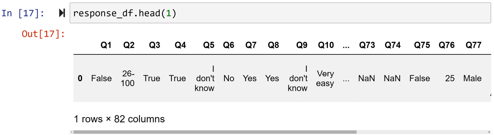
Figure 9.6 – Showing the first row of the cleaned response_df

In this example, we took steps to ensure that the second characteristic of level I data cleaning has been met since the dataset was in good shape in terms of the first and third characteristics.

So far, you've learned and practiced, by example, some examples of data cleaning. In the next chapter, we will learn about and see examples of level II data cleaning.

Summary

Congratulations on your excellent progress. In this chapter, we introduced you to three different levels of data cleaning and their relevance, along with the goals and tools of analytics. Moreover, we covered level I of data cleaning in more detail and practiced dealing with situations where this type of data cleaning is needed. Finally, by looking at three examples, we used the programming and analytics skills that we had developed in the previous chapters to effectively preprocess example datasets and meet the examples' analytical goals.

In the next chapter, we will focus on level II of data cleaning. Before moving forward and starting your journey on data cleaning level II, spend some time on the following exercises and solidify what you've learned.

Exercises

1. In your own words, describe the relationship between the analytics goals and data cleaning. Your response should answer the following questions:

   a) Is data cleaning a separate step of data analytics and can be done in isolation? In other words, can data cleaning be performed without you knowing about the analytics process?

   b) If the answer to the previous question is no, are there any types of data cleaning that can be done in isolation?

   c) What is the role of analytic tools in the relationship between analytic goals and data cleaning?

2. A local airport that analyzes the usage of its parking has employed a Single-Beam Infrared Detector (SBID) technology to count the number of people who pass the gate from the parking area to the airport.

   As shown in the following diagram, an SBDI records every time the infrared connection is blocked, signaling a passenger entering or exiting:

Figure 9.7 – An example of a Single-Beam Infrared Detector (SBID)

Unfortunately, the person who installed the SBID was not up to date with the latest and greatest database technology, so they have set up the system in a way that the recorded date of each day is stored in an Excel file. The Excel files are named after the days the records were created. You have been hired to help and analyze the data. Your manager has given you access to a zipped file called SBID_Data.zip. This zipped file contains 14 files, each containing the data of one day between October 12, 2020, and October 25, 2020. Your manager has informed you that due to security reasons, she cannot share all 3,000 files with you. She has asked you to do the following for the 14 files she has shared with you:

a) Write some code that can automatically consolidate all the files into one Pandas DataFrame.

b) Create a bar chart that shows the average airport passenger traffic per hour.

c) Label and describe the data cleaning steps you did in this exercise.