Chapter 3: Data – What Is It Really?

This chapter presents a conceptual understanding of data and introduces data concepts, definitions, and theories that are essential for effective data preprocessing. First, the chapter demystifies the word "data" and presents a definition that best serves data preprocessing. Next, it puts forth the universal data structure, table, and the common language everyone uses to describe it. Then, we will talk about the four types of data values and their significance for data preprocessing. Finally, we will discuss the statistical meanings of the terms information and pattern and their significance for data preprocessing.

The following topics will be covered in this chapter:

• What is data?
• The most universal data structure: a table
• Types of data values
• Information versus pattern

Technical requirements

You will be able to find all of the code examples that are used in this chapter, as well as the dataset, in Chapter 3's GitHub repository:

https://github.com/PacktPublishing/Hands-On-Data-Preprocessing-in-Python/tree/main/Chapter03

What is data?

What is the definition of data? If you ask this question of different professionals in various fields, you will get all kinds of answers. I always ask this at the beginning of my data-related courses, and I always get a wide range of answers. The following are some of the common answers that my students have given when this question was asked:

• Facts and statistics
• Collections of records in databases
• Information
• Facts, figures, or information that's stored in or used by a computer
• Numbers, sounds, and images
• Records and transactions
• Reports
• Things that computers operate on

All of the preceding answers are correct, as the term data in different situations could be used to refer to all of the preceding. So, next time someone says we came to XYZ conclusions after analyzing the data, you know what your first question should be, right? Yes, the next question would be to understand exactly what they mean by "data."

So, let me try and answer this question, What is meant by data?, with regards to this book, Hands-On Data Preprocessing Using Python.

From a data preprocessing perspective, we need to step back and provide a more general and all-encompassing definition. Here, we define data as symbols or signs representing a measurement or model of reality. These symbols and signs are in themselves useless until used with regard to higher-level conventions and understandings (HLCUs).

I like two things about the previous definition:

• First, the definition is universal and encompasses all of the kinds of data you can imagine, including the ones my students offered.
• Second, it verbalizes an implicit assumption in all the other definitions – the existence of HLCUs.

Without HLCUs, data is a pile of meaningless symbols and signs.

Note:

A quick note before moving forward – I am going to use "HLCU" a lot in this chapter, so maybe read its definition a few more times to commit it to memory.

Before the advent of AI, we could safely say the HLCU is almost always human language and comprehension. However, now algorithms and computers are becoming a legitimate, and in some aspects more powerful, HLCU of data.

Why this definition?

For data preprocessing, the very first thing you want to decide is the HLCU you will be using. That is, what HLCU are you preparing your data for? If the data is being prepared for human comprehension, the result will be very different than when the data is prepared for computers and algorithms. Not only that, the HLCU might be different from one algorithm to another.

One of the stark differences between human comprehension and computers as HLCUs is that humans cannot digest more than two to three dimensions at a time. Being able to process data with larger dimensions and size is the hallmark of algorithms and computers.

There is an important and distinctive relationship between the two HLCUs that needs to be understood for effective data preprocessing. Let's learn about the DIKW pyramid first, and I will use this to discuss that distinction.

DIKW pyramid

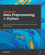
Data, Information, Knowledge, and Wisdom (DIKW), also known as the wisdom hierarchy or data pyramid, shows the relative importance and abundance of each of these four elements. The following figure shows transactional steps between the stages, namely processing, cognition, and judgment. Moreover, the figure specifies that only wisdom, which is the rarest and most important element, is of the future, and the three other elements, namely knowledge, information, and data, are of the past.

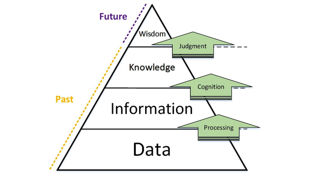
Figure 3.1 – DIKW pyramid

The definition of the four elements is presented as follows:

• Data: A collection of symbols – cannot answer any questions.
• Information: Processed data – can answer the questions who, when, where, and what.
• Knowledge: Descriptive application of Information – can answer the question how.
• Wisdom: Embodiment of Knowledge and appreciation of why.

While the DIKW pyramid is referenced again and again in many data analytics books and articles, you can see that the pyramid's HLCU is human language and comprehension. That is why even though the pyramid makes a lot of sense, it is still not completely applicable to data analytics.

An update to DIKW for machine learning and AI

I have updated the DIKW pyramid to Data, Dataset, Pattern, and Action (DDPA) as I believe it pertains better to Machine Learning (ML) and artificial intelligence.

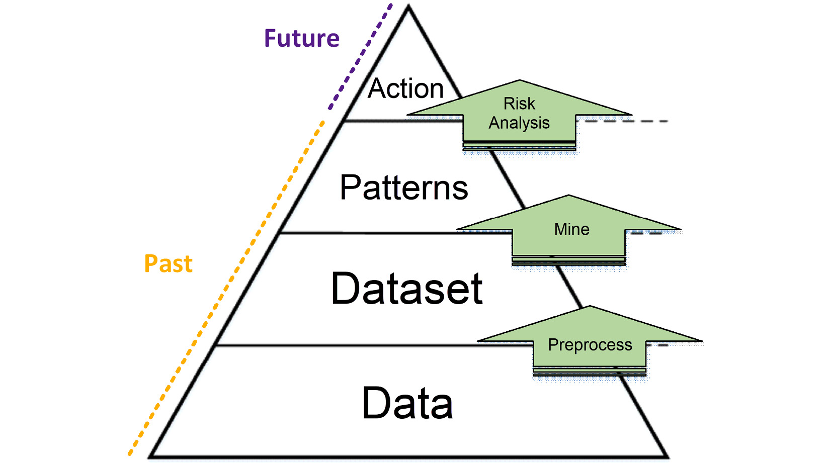
Figure 3.2 – DDPA pyramid

The definitions of all four elements of DDPA are presented as follows:

• Data: All possible data from across all the data resources
• Dataset: A relevant collection of data selected from all the available data sources, cleaned and organized for the next step
• Patterns: The interesting and useful trends and relationships within the dataset
• Action: The decision made, which is informed by the recognized patterns

Let's go through the three transactional steps between the four elements of the DDAP pyramid:

1. Preprocess is to select the relevant data and prepare it for the next step.
2. Mine is applying data mining algorithms to the data in search of patterns.
3. Lastly, risk analysis is the step to consider the uncertainty of the recognized patterns and arrive at a decision.

The DDPA pyramid shows the pivotal role of data preprocessing as the goal of being able to drive action from data. Preprocessing of the data is perhaps the most important step from D to A (Data to Action). Not all the data in the world will be useful for driving action in specific cases, and the data mining algorithms that are developed are not capable of finding patterns in all types of data.

An update to DIKW for data analytics

It is important to remember that data preprocessing in no way pertains only to ML and artificial intelligence. When analyzing data using data visualization, data preprocessing also has a pivotal but slightly different role.

Neither the DIWK nor the DDPA pyramid can be applied well to data analytics. As mentioned earlier, DIWK was designed for human language and comprehension, and I created DDPA for algorithms and computers, so it is better suited for machine learning and artificial intelligence. However, data analytics falls between the two ends of this spectrum, where both humans and computers are involved.

I have designed another pyramid specifically for data analytics and its unique HLCUs. As the HLCUs of data analytics are both humans and computers, the Data, Dataset, Visualization, and Wisdom (DDVW) pyramid is a combination of the other two pyramids.

Figure 3.3 – DDVW pyramid

The definitions of all four elements of DDVW are presented as follows:

• Data: All possible data from across all the data resources
• Dataset: A relevant collection of data selected from all the available data sources and organized for the next step
• Visualization: The comprehensible presentation of what has been found in the dataset (similar to Knowledge in DIKW – descriptive application of Information)
• Wisdom: Embodiment of Knowledge and appreciation of why (the same as Wisdom in DIKW)

While the first transactional step of DDVW is similar to that of DDPA (both are preprocessing), the second and third are different. The second transactional step of DDVW is to analyze. That is what a data analyst does – use technology to do the following:

1. Explore the dataset.
2. Test the hypothesis.
3. Report the relevant findings.

The most understandable way to report the findings for the decision-maker is visualization. A decision-maker will understand the visualization and use judgment (the third transaction step of DDVW) to develop wisdom.

Data preprocessing for data analytics versus data preprocessing for machine learning

Data preprocessing is a pivotal step for both data analytics and machine learning. However, it is important to recognize the preprocessing that is done for data analytics is very different from that of machine learning.

As seen in DDPA, the only HLCU for machine learning is computers and algorithms. However, as shown in DDVW, the HLCU of data analytics is first computers and then it switches over to humans. So, in a sense, the data preprocessing that is done for machine learning is simpler, as there is only one HLCU to consider. However, when the data is preprocessed for data analytics, both HLCUs need to be considered.

Now that we have a good understanding of what we mean by data, let's switch gears and learn some important concepts surrounding data. The next concept we will discuss helps us distinguish between data analytics and machine learning even further.

The three Vs of big data

A very useful concept that helps to distinguish between machine learning and data analytics is the three Vs of big data. The three Vs are volume, variety, and velocity.

The general rule of thumb is that when your data has high volume, high variety, and high velocity, you want to consider machine learning and AI over data analytics. As a general rule, this could be true, but if and only if you have high volume, high variety, and high velocity after appropriate data preprocessing. So, data preprocessing plays a major role, and that will be explained in more detail after going over the three Vs:

• Volume: The number of data points that you have. You can roughly think of data points as rows in an Excel spreadsheet. So, if you have many occurrences of the phenomena or entities that you have collected, your data is of high volume. For example, if Facebook was interested in studying its users in the US, the volume of this data would be the number of Facebook users in the US. Pay attention – the data point in this study of Facebook is US users of the platform.
• Variety: The number of different sources of data you have that give you fresh new information and perspective about the data points. You can roughly think of the variety of your data as the number of columns you have in an Excel spreadsheet. Continuing the Facebook example – Facebook has information such as the name, date of birth, and email of its users. But Facebook could also add variety to this data by including behavior columns, such as the number of visits in the last week, the number of posts, and many more. The variety does not stop there for Facebook, as it also owns other services that users may be using, such as Instagram and WhatsApp. Facebook could add variety by including the behavior data of the same users from the other services.
• Velocity: The rate at which you are getting new data objects. For instance, the velocity of Facebook US users' data is much higher than the velocity of Facebook's employees' data. But the velocity of Facebook US users' data is much lower than Facebook's US post's data. Pay attention to what changes the velocity of data – it is how often the phenomena or the entities you are collecting happen.

The importance of the three Vs for data preprocessing

Data analytics that heavily involves human comprehension cannot accommodate data that has high volume, high variety, and high velocity. However, sometimes the high Vs are happening due to the lack of proper data preprocessing. One important element of successful data preprocessing is to include data that is relevant to the analysis. Just because you have to dig through data with high Vs to prepare a dataset, that is not enough of a reason to give up on data analytics in favor of machine learning.

Next, we will move on from pure concepts to begin talking about the data itself and the way we normally organize it.

The most universal data structure – a table

Regardless of the complexity and high Vs of your data, and even regardless of you wanting to do data visualization or machine learning, successful data preprocessing always leads to one table. At the end of successful data preprocessing, we want to create a table that is ready to be mined, analyzed, or visualized. We call this table a dataset. The following figure shows you a table with its structural elements:

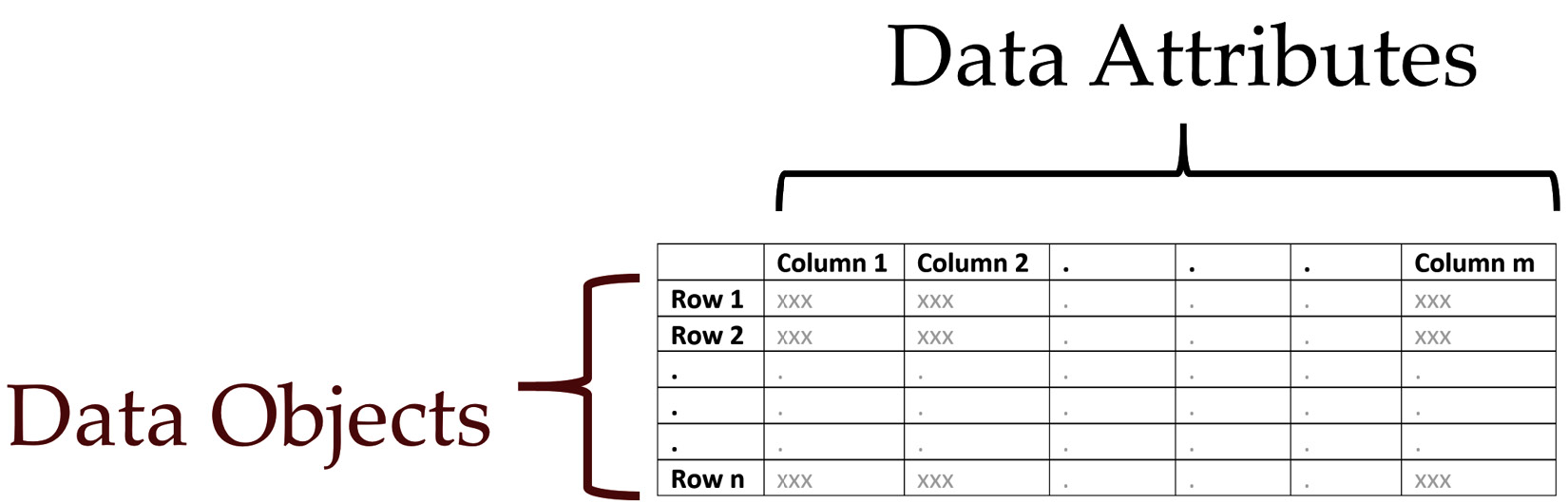
Figure 3.4 – Table data structure

As shown in the figure, for data analytics and machine learning, we use specific keywords to talk about the structure of a table: data objects and data attributes.

Data objects

I'm sure you have seen and successfully made sense of so many tables and created so many of them as well. I bet many of you would have never paid attention to the conceptual foundations of the table that allows you to create them and make sense of them. The conceptual foundation of a table is its definition of the data object.

Data objects are known by many different names, such as data points, rows, records, examples, samples, tuples, and many more. However, as you know for a table to make sense, you need the conceptual definition of data objects. You need to know for what phenomena, entity, or event the table is presenting values.

The definition of the data object is the entity, concept, phenomena, or event that all of the rows share. For instance, the entity that holds a table of information about customers together is the concept of the "customer." Each row of the table represents a customer and gives you more information about them.

The definition of the data object for some tables is straightforward, but not always. The very first concept you want to figure out when reading a new table is what the assumed definition of data objects for the table is. The best way you can go about this is to ask the following question: what is the one entity that all of the columns in the table describe? Once you have found that one entity, bingo! You have found the definition of the data object.

Emphasizing the importance of data objects

For data preprocessing, the definition of the data objects becomes more important. A lot of the time, the data analyst or machine learning engineer is the one that needs to first envision the end table that data needs to be preprocessed into. This table needs to be both realistic and useful. In the following two paragraphs I will address what I mean by realistic and useful:

• Realistic: The table needs to be realistic in the sense that you have the data, technology, and access to create the table. For instance, I can imagine if I had a table of data about newly married couples, with columns for the first month of their marriage such as the number of times they kissed, or the number of times they were passive-aggressive toward each other, I could build a universal model that could tell couples whether their marriage was going to be successful or not. In this case, the definition of data objects is newly married couples, and all of the imagined columns describe this entity. However, realistically coming up with such a table is very difficult. Incidentally, John Gottman from the University of Washington and James Murry from Oxford University did create this model, but only with 700 couples who were willing to be recorded while they were discussing contentious topics and were willing to share the updates on their relationship with the researchers.
• Useful: The imagined table also needs to be useful for analytics goals. For instance, suppose that somehow we have access to the video recordings of the first month of all of the newly married couples. These recordings are stored in separate files, organized by day. So, we set out to preprocess the data and count the number of kisses and the number of passive-aggressive incidents for each recording and store them in a table. This table's data object definition is the video recording of one day of a newly married couple. Is this data object definition useful for the analytics goals of predicting the success of couples? No, the data needs to be collated differently so the data objects are the newly married couples.

Data attributes

As shown in Figure 3.4, the columns of a table are known as attributes. Different names such as columns, variables, features, and dimensions might be used instead of attributes. For example, in math, you are more likely to refer to "variables" or "dimensions," whereas, in programming, you more often refer to "variables."

Attributes are describers of the data objects in a table. Each attribute describes something about all of the data objects. For instance, in the table we envisioned for the newly married couples, the number of kisses and the number of passive-aggressive incidents are the attributes of that table.

Types of data values

For successful data preprocessing, you need to know the different types of data values from two different standpoints: analytics and programming. I will review the types of data values for both standpoints and then share with you their relationships and their connections.

Analytics standpoint

There are four major types of values from analytics standpoints: nominal, ordinal, interval-scaled, and ratio-scaled. In the literature, these four types of values are under four types of data attributes. The reason is that the types of values for each attribute must remain the same, therefore, you can extrapolate value types to attribute types.

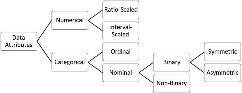
Figure 3.5 – Types of data attributes

The preceding figure shows the tree of attribute types. The four mentioned types are in the middle. As you can see in the tree, Nominal and Ordinal attributes are called Categorical (or qualitative) attributes, whereas Interval-Scaled and Ratio-Scaled attributes are called Numerical (or quantitative).

Nominal attributes

As the name suggests, this type of attribute refers to the naming of objects. There is no other information that this attribute describes apart from a simple set of letters and symbols that act as a name of the object or a category of the object.

A prominent example of a nominal attribute is gender when data objects are individuals. While this attribute may be shown differently, the information it contains is a simple name for two categories of humans. I have seen this information represented in many ways. The following table shows all the different ways the nominal attribute gender can be presented. Regardless of how the categories are presented, the information that is gathered by this category is that an individual is either male or female.

Figure 3.6 – Different presentations of the nominal attribute gender

Other examples of nominal attributes when the data objects are individuals are hair color, skin color, eye color, marital status, or occupation. What is important to remember about nominal attributes is that they do not contain any other information than just names.

Ordinal attributes

On the other hand, ordinal attributes, as the name suggests, contain more information that pertains to some types of order. For instance, when the data objects are individuals, the level of education is a prime example of an ordinal attribute. While high school, bachelor's, master's, and doctoral are names that refer to the names of education degrees, there is a well-recognized order between all of them.

No one could logically give any order to the importance, value, or recognition between the values of a nominal attribute such as gender. However, it is quite acceptable to assume the number of resources (time, money, energy) someone has spent to get a bachelor's degree is more than a high school degree.

Other examples of ordinal attributes are course letter grades (A, B, C, D), professional rankings (Assistant Professor, Associate Professor, and Full Professor), and survey rates (highly agree, agree, neutral, disagree, highly disagree).

So far, we know that ordinal attributes can contain more information than nominal attributes. At the same time, ordinal attributes are themselves limited in the sense that they do not contain how much each possible value of an ordinal attribute is different from the other. For instance, we know that Individual A, who has a doctorate, might be able to deal with research projects better than Individual B, who has a bachelor's degree. However, we cannot say Individual A will finish a research task 20 hours faster than Individual B. Simply put, ordinal attributes do not contain information that allows for interval comparison between data objects.

Interval-scaled attributes

These attributes contain more information than ordinal attributes, as they allow for interval comparison between data objects. By moving from ordinal attributes to interval attributes, we also move from symbols and categories to numbers (categorical attributes to numerical attributes). With numbers comes the capability to know how much difference exists between data objects. For instance, when data objects are individuals, height is an interval attribute. For instance, Roger Federer's height is 6'1", and everyone will agree that he is shorter than Juan Martín del Potro by 5", as del Potro's height is 6'6".

Another example of an interval attribute when the data objects are individuals is weight. The measurement of temperature in Fahrenheit or Celcius when the data objects are days is also an example of an interval-scaled attribute.

The limitation of interval attributes is that we cannot use them for a ratio-based comparison. For instance, will we ever be able to say an individual is twice as tall as the other individual? You might be thinking yes. But the answer is no. The reason is that there is no meaningful zero for the concept of human tallness. That is to say, there is no individual whose height is zero.

The shortest man in the world is documented to have been Chandra Bahadur Dangi and his height was 1'10". Also, Robert Wadlow, with a height of 8'3", is reported to have been the tallest man in the world. To put things into perspective, consider the following figure, where you can compare the average heights with the recorded extremes:

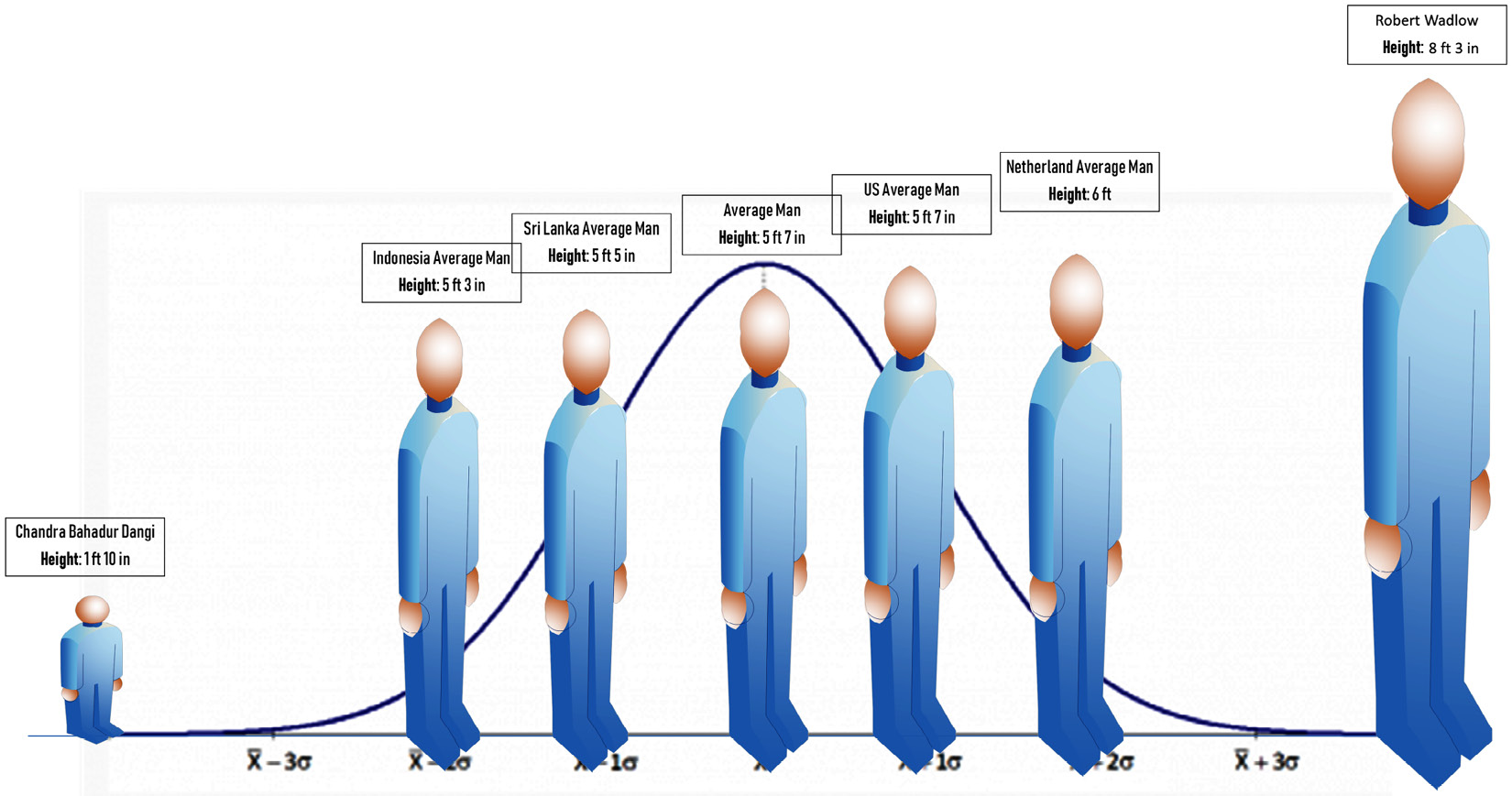
Figure 3.7 – The spectrum of men's heights

Looking at the two extremes might challenge our preconceptions about height. However, if you remove the two extremes, you will start feeling more comfortable. The reason for this discomfort is that tallness is an interval attribute for our brain. We do not come across very tall people or very short people in our daily lives. Although it will completely make sense to most people if you say you are 2 inches taller than another person, it would not make sense if you were to claim you are more than 3 times taller than the shortest man in the world.

For instance, since I am 6'3", you will believe I am 3.41 times taller than the shortest man in the world. While the mathematics of this calculation is correct ((6*12+3) / (6*1+10) = 3.41), you cannot say I am 3.41 times taller than the shortest man in the world, because the shortest man in the world is the zero in the concept of human tallness. At best, you can say I am 3.41 times taller an object than Chandra Bahadur Dangi. But to be able to do that, you had to change the definition of the data object from an individual to an object.

Even if you have a roommate that is a very short person and you see him every day, mathematically, it does not make sense to have a multiplication of tallness as there is no absolute zero. There is no individual you could ascribe the value zero to for their tallness.

Ratio-scaled attributes

When we move to ratio-scaled attributes, the last limitation, which was the incapability to multiply or divide values for interval-scaled attributes, is also removed, as we can find an inherent zero for them. For instance, when our data objects are individuals, monthly income is an example of a ratio-scaled attribute. We can imagine an individual with no monthly income. For instance, it completely makes sense if you were to report that your dad makes twice what you make every month. Another example of a ratio-scaled attribute is the temperature in kelvin when the definition of data object is a day.

Binary attributes

Binary attributes are nominal attributes with only two possibilities. For instance, the gender you are assigned at birth is either male or female, so Sex Assigned At Birth (SAAB) is a binary attribute.

There are two types of binary attributes: symmetric and asymmetric. Symmetric binary attributes, such as SAAB, are where either of the two possibilities happens as frequently and carries the same level of importance for our analysis.

However, one of the two possibilities of asymmetric binary attributes happens less frequently and is normally more important. For instance, the result of a COVID test is an asymmetric binary attribute, where the positive results happen less often but are more important in our analysis.

You might think that symmetric binary attributes are more common than asymmetric binary attributes, however, that is far from the reality. Try to think of other symmetric binary attributes, and email them to me if you find a few good ones.

Conventionally, the rarer possibility of a binary attribute is denoted by a positive (or one), whereas the more common possibility is denoted by a negative (or zero).

Understanding the importance of attribute types

As analytic methods become more complex, it will become easier to make mistakes and never know about them. For instance, you might inadvertently input an integer-coded nominal attribute into an algorithm that regards these values as real numbers. What you have done is to input randomly assumed relationships between the data objects that have no basis in reality to a model that cannot think for itself. See Exercise 5 for an example of this.

Programming standpoint

By and large, values are either known as numbers, strings, or Booleans for computers. Numbers might be recognized as integers or floating points, but that is it.

Integers are whole numbers from zero to infinity. For instance, 0, 1, 2, 3, and so on are all integer values. Floating points are numbers. They can be positive or negative and have decimal points. For instance, 1.54, -25.1243, and 0.1 are all floating points.

I hope you see the challenge here – from an analytics perspective, you may have nominal or ordinal attributes but computers can only show them as strings. Similarly, from an analytics perspective, you may have ratio-scaled or interval-scaled attributes but computers can only show them as numbers. The only complete match between programming value types and analytics value types is binary attributes that can be presented completely with Boolean values.

The following table presents a mapping of attribute (value) types between analytics and programming perspectives. As you are developing skills to effectively preprocess data, this mapping should become second nature to you. For instance, you want to understand your options of presenting an ordinal attribute with Booleans, strings, or integers, and what each option would entail (see exercise 6 in the Exercise section).

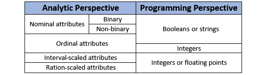
Figure 3.8 – Mapping of value types between analytics and programming

So far in this chapter, we covered the definition of data and also the types of data attributes. Now, we are going to talk about two high-level and important concepts that are essential for successful data preprocessing: information and pattern.

Information versus pattern

Before finishing this chapter, which aims to arm you with all the necessary definitions and concepts needed for data preprocessing, we need to cover two more concepts: information and pattern.

Understanding everyday use of the word "information"

First, I need to bring your attention to two specific and yet very different functions of the term information. The first one is the everyday use of "information," which means "facts or details about somebody or something." This is how the Oxford English Dictionary defines information. However, while statisticians also employ this function of the word, sometimes the term information serves another purpose.

Statistical use of the word "information"

The term "information" could also refer to the value variation of one attribute across the population of a data object. In other words, information is used to refer to what an attribute adds to space knowledge of a population of data objects. Let's explore an example dataset, customer_df, as shown in the following screenshot. The dataset is pretty small and has 10 data objects and 4 attributes. The definition of the data object for the following dataset is customers.

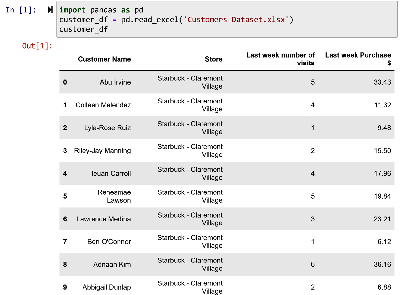
Figure 3.9 – Reading Customer Dataset.xlsx and seeing its records

We will talk about this dataset as we go over the following subsections.

Statistical information for categorical attributes

Customer Name is a nominal attribute, and the value variation this attribute adds to the space knowledge of this dataset is the maximum possible for a nominal attribute. Each data object has a completely different value under this attribute. Statistically speaking, the amount of information this attribute has is very high.

The case of the attribute store is the opposite. This attribute adds the minimal possible information a nominal attribute may add – that is, the value for every data object under this attribute is the same. When this happens, you should remove the attribute and see whether you can perhaps update the definition of the data objects. If we change the definition of the data objects to Starbucks customers of Claremont Village store, we have retained the information and we can safely remove the attribute.

Statistical information for numerical attributes

The matter of statistical information for numerical attributes is a little bit different. For numerical attributes, you can calculate a metric called variance to drive how much information each numerical attribute has. Variance is a statistical metric that captures the spread between a collection of numbers. It is calculated by the summation of the squared distances of each number from the mean of all the numbers. The higher the variance of an attribute, the more information the attribute has. For instance, the variance for the Last week number of visits attribute is 3.12, and the variance for the Last week Purchase $ attribute is $109.63. Calculating the variance using Pandas is very easy. See the following screenshot:

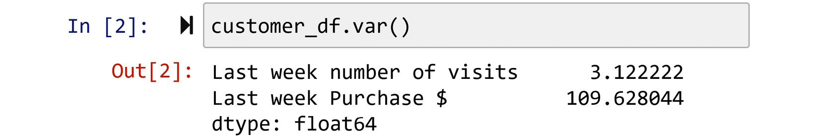
Figure 3.10 – Calculating the variance for the numerical attributes of customer_df

We would be able to say the Last week Purchase $ attribute has more information than the Last week number of visits attribute if the attributes had a similar range. However, the attributes have a completely different range of values, and it makes the two variance values incomparable. There is a way to get around this issue – we can normalize both the attributes and then calculate their variance. Normalization is a concept that we will cover later in this book.

Data redundancy – attributes presenting similar information

We call an attribute redundant if the variation of its value across the data objects of a dataset is too similar to that of another attribute. To check data redundancy, you can draw a scatterplot for the variables you suspect are presenting similar information. For instance, the following screenshot has drawn the scatterplot of the two numerical attributes of customer_df:

Figure 3.11 – Drawing the scatterplots for the two attributes, Last week number of visits and Last week Purchase $

You can see that it seems that with the increase in the number of visits, the purchase has also increased.

Correlation coefficient to investigate data redundancy

You can also use the correlation coefficient to investigate data redundancy. A correlation coefficient value falls between -1 and 1. When the value is close to zero, it means the two attributes are not showing similar information. When the correlation coefficient between two numerical attributes is closer to both ends of the spectrum (-1 or +1), it shows that the two attributes are showing similar statistical information and perhaps one of them is redundant. When two attributes have a significant and positive correlation coefficient (greater than 0.7), that means if the value of one attribute increases the value of the other attribute will also increase. On the other hand, when two attributes have a significant and negative correlation coefficient (smaller than -0.7), that means the increase of one attribute leads to the decrease of the other.

The following screenshot has used .corr() to calculate the correlation coefficient between the numerical attributes in customer_df:

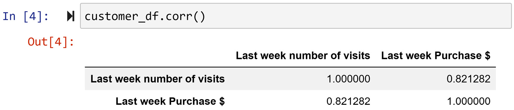
Figure 3.12 – Finding the correlation coefficients for the pairs of numerical attributes in customer_df

The correlation coefficient is 0.82, which is considered high, indicating one of the two numerical attributes might be redundant. The cut-off rule of thumb for high correlation is 0.7 – that is, if the correlation coefficient is higher than 0.7 or lower than -0.7, there might be a case of data redundancy.

Now that we have a good understanding of the term information, let's turn our attention to the term pattern.

Statistical meaning of the word "pattern"

While the statistical meaning of "information" is the value variation of one attribute across the data objects of a dataset, the statistical meaning of "pattern" is about the value variation of more than one attribute across the data objects. Every specific value variation of more than one attribute across the data objects of a dataset is called a pattern.

It is important to understand that most patterns are neither useful nor interesting. It is the job of a data analyst to find interesting and useful patterns from the data and present them. Also, it is the job of an ML engineer to streamline a model that collects the expected and useful patterns from the data and makes calculated decisions based on the collected patterns.

Example of finding and employing a pattern

The relationship we found between the two numerical attributes of customer_df in the following situation could be considered as useful.

The manager of the Starbucks store in Claremont Village made a huge blunder and accidentally removed the values of Last week Purchase $ for 10 customers from the records, but luckily she knows about the power of data analytics, and the Last week number of visits attribute is intact. The following screenshot shows the second part of this data:

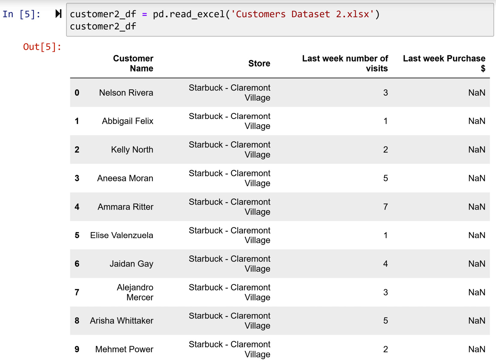
Figure 3.13 – Reading Customer Dataset 2.xlsx and seeing its records

The manager of the store, after having seen the high correlation between Last week number of visits and Last week Purchase $, can use simple linear regression to extract, formulate, and package the pattern from the 10 customers with all of the data. After the regression model is trained, the manager can use it to estimate the purchase $ for the customers that have missing values.

Simple linear regression is a statistical method where the values of one numerical attribute (X) are linked to the values of another numerical attribute (Y). In statistical terms, when we observe a close relationship between two numerical attributes, we may investigate to see whether X can predict Y.

The following screenshot illustrates the application of .regplot() from the Seaborn module to visualize the linear regression line that has fitted to the data of the first 10 customers in customer_df:

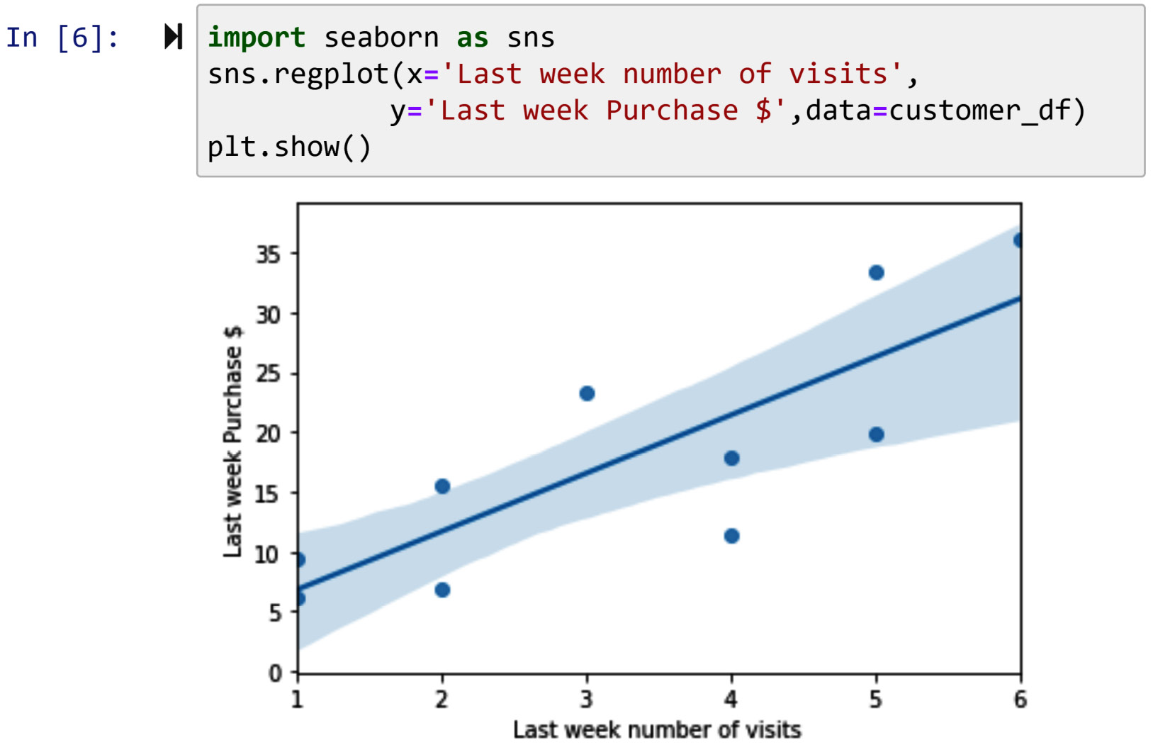
Figure 3.14 – Using .regplot() to show the regression line between the two attributes, Last week number of visits and Last week Purchase $

Installation of the Seaborn module

If you have never used the Seaborn module, you have to install it first. Installing it on Anaconda is very simple. Open a chunk of code in your Jupyter notebook and run the following line of code:

conda install seaborn

The equation of the fitted regression model is shown as follows:

Now, this equation allows us to estimate the missing values of customer2_df. The following screenshot shows the preceding equation is applied to customer2_df to calculate the missing values:

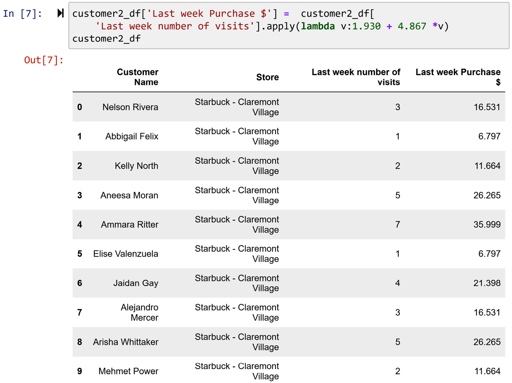
Figure 3.15 – Using the extracted pattern (regression equation) and .apply() function to estimate and replace the missing values

So, this way the manager of the Starbucks store in Claremont Village was able to save the day and replace the missing values with estimated values that are based on a reliable pattern found in the data.

Before moving on, let me acknowledge that we have not yet covered linear regression in this book (we will do this in Chapter 6, Prediction). However, in this example, we used linear regression to showcase an instance of extracting and using the pattern in a dataset for an analytic situation. We did this in the interest of understanding what we mean by "useful patterns," and extracting and packaging patterns for later use.

Summary

Congratulations on finishing this chapter. You have now equipped yourself with an essential understanding of data, data types, information, and pattern. Your understanding of these concepts will be vital in your journey to successful data preprocessing.

In the next chapter, you will learn about the important roles databases play for data analytics and data preprocessing. However, before moving on to the next chapter, take some time and solidify and improve your learning using the following exercises.

Exercises

1. Ask five colleagues or classmates to provide a definition for the term data.

   a) Record these definitions and notice the similarities among them.

   b) In your own words, define the all-encompassing definition of data put forth in this chapter.

   c) Indicate the two important aspects of the definition in b).

   d) Compare the five definitions of data from your colleagues with the all-encompassing definitions and indicate their similarities and differences.

2. In this exercise, we are going to use covid_impact_on_airport_traffic.csv. Answer the following questions. This dataset is from Kaggle.com – use this link to see its page:

   https://www.kaggle.com/terenceshin/covid19s-impact-on-airport-traffic

   The key attribute of this dataset is PercentOfBaseline, which shows the ratio of air traffic in a specific day compared to a pre-pandemic time range (February 1 to March 15, 2020).

   a) What is the best definition of the data object for this dataset?

   b) Are there any attributes in the data that only have one value? Use the .unique() function to check. If there are, remove them from the data and update the definition of the data object.

   c) What type of values do the remaining attributes carry?

   d) How much statistical information does the PercentOfBaseline attribute have?

3. For this exercise, we are going to use US_Accidents.csv. Answer the following questions. This dataset is from Kaggle.com – use this link to see its page:

   https://www.kaggle.com/sobhanmoosavi/us-accidents

   This dataset shows all the car accidents in the US from February 2016 to December 2020.

   a) What is the best definition of the data object for this dataset?

   b) Are there any attributes in the data that only have one value? Use the .unique() function to check. If there are, remove them from the data and update the definition of the data object.

   c) What type of values do the remaining attributes carry?

   d) How much statistical information do the numerical attributes of the dataset carry?

   e) Compare the statistical information of the numerical attributes and see whether any of them are a candidate for data redundancy.

4. For this exercise, we are going to use fatal-police-shootings-data.csv. There are a lot of debates, discussions, dialogues, and protests happening in the US surrounding police killings. The Washington Post has been collecting data on all fatal police shootings in the US. The dataset available to the government and the public alike has date, age, gender, race, location, and other pieces of situational information related to these fatal police shootings. You can download the last version of the data from https://github.com/washingtonpost/data-police-shootings.

   a) What is the best definition of the data object for this dataset?

   b) Are there any attributes in the data that only have one value? Use the .unique() function to check. If there are, remove them from the data and update the definition of the data object.

   c) What type of values do the remaining attributes carry?

   d) How much statistical information do the numerical attributes of the dataset carry?

   e) Compare the statistical information of the numerical attributes and see whether any of them are a candidate for data redundancy.

5. For this exercise, we will be using electricity_prediction.csv. The following screenshot shows the five rows of this dataset and a linear regression model created to predict electricity consumption based on the weekday and daily average temperature:
   

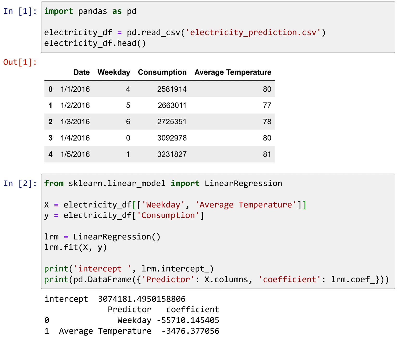
   Figure 3.16 – Screenshot for Exercise 5

   a) The regression model that is derived from the data is presented as follows:

   

   b) What is the fundamental mistake in this analysis? Describe it and provide possible solutions for it.

6. For this exercise, we will be using adult.csv. We used this dataset extensively in Chapter 1, Review of the Core Modules NumPy and Pandas and Chapter 2, Review of Another Core Module – Matplotlib. Read the dataset using Pandas and call it adult_df.

   a) What type of values does the education attribute carry?

   b) Run adult_df.education.unique(), study the results, and explain what the code does.

   c) Based on your understanding, order the output of the code you ran for b).

   d) Run pd.get_dummies(adult_df.education), study the results, and explain what the code does.

   e) Run adult_df.sort_values(['education-num']).iloc[1:32561:1200], study the results, and explain what the code does.

   f) Compare your answer to c) and what you learned from e). Was the order you came up with in c) correct?

   g) The education attribute is an ordinal attribute – translating an ordinal attribute from an analytic perspective to a programming perspective involves choosing between Boolean representation, string representation, and integer representation. Choose which choice has been made for the three following representations of the education attribute:

   adult_df.education

   pd.get_dummies(adult_df.education)

   adult_df['education']

   h) Each choice has some advantages and some disadvantages. Select which programing data representation each following statement describes:

   If an ordinal attribute is presented using this programming value representation, no bias or assumptions are added to the data, but algorithms that work with numbers cannot use the attribute.

   If an ordinal attribute is presented using this programming value representation, the data can be used by algorithms that only take numbers, but the size of the data becomes bigger and there may be concerns for computational costs.

   If an ordinal attribute is presented using this programming value representation, there will be no size or computational concerns, but some statistical information that may not be true is assumed and it may create bias.

References

John M. Gottman, James D. Murray, Catherine C. Swanson, Rebecca Tyson, and Kristin R. Swanson. The Mathematics of Marriage: Dynamic Nonlinear Models. MIT Press, 2005.