Chapter 10: Data Cleaning Level II – Unpacking, Restructuring, and Reformulating the Table

In level I data cleaning, we were only concerned about the neat and codable organization of our dataset. As we mentioned previously, level I data cleaning can be done in isolation, without having to keep an eye on what data will be needed next. However, level II data cleaning is deeper. It is more about preparing the dataset for analysis and the tools for this process. In other words, in level II data cleaning, we have a dataset that is reasonably clean and is in a standard data structure, but the analysis we have in mind cannot be done because the data needs to be in a specific structure due to the analysis itself, or the tool we plan to use for the analysis.

In this chapter, we will look at three examples of level II data cleaning that tend to happen frequently. Pay attention to the fact that, unlike level I data cleaning, where the examples were merely a source of data, the examples for level II date cleaning must be coupled with an analytical task.

In this chapter, we're going to cover the following main topics:

• Example 1 – unpacking columns and reformulating the table
• Example 2 – restructuring the table
• Example 3 – level I and II data cleaning

Technical requirements

You can find all the code and the dataset for this book in this book's GitHub repository: https://github.com/PacktPublishing/Hands-On-Data-Preprocessing-in-Python. You can find the Chapter10 directory in this repository and download the code and the data for a better learning experience.

Example 1 – unpacking columns and reformulating the table

In this example, we will use the level I cleaned speech_df dataset to create the following bar chart. We cleaned this DataFrame in the Example 1 – unwise data collection section of Chapter 9, Data Cleaning Level I – Cleaning Up the Table. The level I cleaned speech_df database only has two columns: FileName and Content. To be able to create the following visual, we need columns such as the month of the speech and the number of times the four words (vote, tax, campaign, and economy) have been repeated in each speech. While the level I cleaned speech_df dataset contains all this information, it is somewhat buried inside the two columns.

The following is a list of the information we need and the column of speech_df that this information is stored in:

• The month of the speech: This information is in the FileName column.
• The number of times the words vote, tax, campaign, and economy have been repeated in each speech: This information is in the Content column:

Figure 10.1 – Average frequency of the words vote, tax, campaign, and economy per month in speech_df

So, for us to be able to meet our analytic goal, which is to create the previous visualization, we need to unpack the two columns and then reformulate the table for visualization. Let's do this one step at a time. First, we will unpack FileName and then we bring our attention to unpacking Content. After that, we will reformulate the table for the requested visualization.

Unpacking FileName

Let's take a look at the values of the FileName column. To do this, you can run speech_df.FileName and study the values under this column. You will notice that the values follow a predictable pattern. The pattern is CitynameMonthDD_YYYY.txt; Cityname is the name of the city where the speech was given, Month is the three-letter version of the month when the speech was given, DD is the one- or two-digit number that represents the day of the month, YYYY is the four digits that represent the year during which the speech was given, and .txt is the file extension, which is the same for all the values.

You can see that the FileName column contains the following information about the speeches in the dataset:

• City: The city where the speech was given
• Date: The date when the speech was given
• Year: The year when the speech was given
• Month: The month when the speech was given
• Day: The day when the speech was given

In the following code, we will use our programming skills to unpack the FileName column and include the preceding information as separate columns. Let's plan our unpacking first and then put it into code. The following are the steps we need to take for the unpacking process:

1. Extract City: Use Month from the CitynameMonthDD_YYYY.txt pattern to extract the city. Based on this pattern, everything that comes before Month is Cityname.
2. Extract Date: Use the extracted Cityname to extract Date.
3. Extract Year, Month, and Day from Date.

Now, let's put these steps into code:

1. Extract City: The following code creates the SeparateCity() function and applies it to the speech_df.FileName Series. The SeparateCity() function loops through the previously created Months list to find the three-letter word that represents a month, which is used for each filename. Then, we can use the.find() function and the slicing capability of the Python strings to return the city's name:

   Months = ['Jan','Feb','Mar','Apr','May','Jun','Jul','Aug','Oct','Sep','Nov','Dec']

   def SeperateCity(v):

       for mon in Months:

           if (mon in v):

               return v[:v.find(mon)]

   speech_df['City'] = speech_df.FileName.apply(SeperateCity)

   Pay Attention!

   Here, we had to use Month as the separator between Cityname and the date. If the naming convention of the files was a bit more organized, we could have done this a bit easier; in the speech_df.FileName column, some days are presented by one digit, such as LatrobeSep3_2020.txt, while some days are presented by two digits, such as BattleCreekDec19_2019.txt. If all the days were presented with two digits, in that they used LatrobeSep03_2020.txt instead of LatrobeSep3_2020.txt, the task of unpacking the column, from a programming perspective, would have been much simpler. For an example, see Exercise 2, later in this chapter.

2. Extract Date: The following code creates the SeparateDate() function and applies it to speech_df. This function uses the extracted city as the starting point, and the .find() function to separate the date from the city:

   def SeperateDate(r):

       return r.FileName[len(r.City):r.FileName.find(    '.txt')]

   speech_df['Date'] = speech_df.apply(SeparateDate,axis=1)

   Every time we work with date information, it is better to make sure that Pandas knows the recording is a datetime programming object so that we can use its properties, such as sorting by date or accessing the day, month, and year values. The following code uses the pd.to_datetime() function to transform the strings that represent the dates to datetime programming objects. To effectively use the pd.to_datetime() function, you need to be able to write the format pattern that the strings that represent dates follow. Here, the format pattern is '%b%d_%Y', which means the string starts with a three-letter month representation (%b), then a digit representation for the day (%d), followed by an underscore (_), and then a four-digit year representation (%Y). To be able to come up with a correct format pattern, you need to know the meaning of each of the directives, such as %b, %d, and so on. Go to https://docs.python.org/3/library/datetime.html#strftime-and-strptime-behavior to find a comprehensive list of these directives:

   speech_df.Date = pd.to_datetime(speech_df.Date,format='%b%d_%Y')

3. Extract Year, Month, and Day from Date: The following code creates the extractDMY() function and applies it to speech_df to add three new columns to each row. Note that the code is taking advantage of the fact that the speech_df column is a datetime programming object that has properties such as .day and .month to access the day and the month for each date:

   def extractDMY(r):

       r['Day'] = r.Date.day

       r['Month'] = r.Date.month

       r['Year'] = r.Date.year

       return r

   speech_df = speech_df.apply(extractDMY,axis=1)

   After running the preceding code snippets successfully, you will have managed to unpack the FileName column of speech_df. Since all of the information that was packed in FileName is not presented under other columns, we can go ahead and remove this column by running the following command:

   speech_df.drop(columns=['FileName'],inplace=True)

   Before unpacking the other column, Content, let's take a look at the state of the data and enjoy looking at the progress we've made. The following screenshot shows the first five rows of the data:

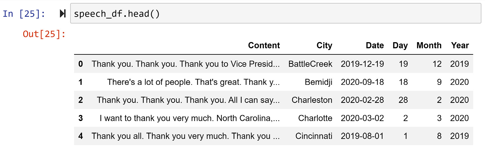
Figure 10.2 – speech_df after unpacking FileName

Now that we have unpacked FileName into five new columns called City, Date, Day, Month, and Year, we have taken one step toward the end goal: we've got access to create the x axis shown in Figure 10.1. Now, we need to pay attention to unpacking the column Content.

Unpacking Content

Unpacking the column Content differs somewhat from unpacking FileName. As the column FileName only had a limited amount of information, we were able to unpack everything this column had to offer. However, the column Content has a lot of information and it could be unpacked in many different ways. However, we only need to unpack a small portion of what is under the column Content; we need to know about the ratio of the usage of four words: vote, tax, campaign, and economy.

We can unpack what we need from the column Content in one step. The following code creates the FindWordRatio() function and applies it to speech_df. The function uses a for loop to add four new columns to the DataFrame, one column for each of the four words. The calculation for each word is simple: the returning value for each word is the total occurrence of the word in the speech (row.Content.count(w)), divided by the total number of words in the speech (total_n_words):

Words = ['vote','tax','campaign','economy']

def FindWordRatio(row):

    total_n_words = len(row.Content.split(' '))

    for w in Words:

        row['r_{}'.format(w)] = row.Content.count(w)/total_n_        words

    return row

speech_df = speech_df.apply(FindWordRatio,axis=1)

The resulting speech_df after running the previous code will have 10 columns, as shown in the following screenshot:

Figure 10.3 – speech_df after extracting the needed information from Content

So far, we have restructured the table, so we are inching closer to drawing Figure 10.1; we've got the information for both the x axis and y axis. However, the dataset needs to be modified further before we can visualize Figure 10.1.

Reformulating a new table for visualization

So far, we have cleaned speech_df for our analytic goals. However, the table we need for Figure 10.1 needs each row to be Donald Trump's speeches in a month while each of the rows in speech_df is one of Donald Trump's speeches. In other words, to be able to draw the visualization, we need to reformulate a new table so that the definition of our data object is Donald Trump's speeches in a month instead of one Donald Trump speech.

The new definition of the Donald Trump's speeches in a month data object is an aggregation of some of the data objects that are defined as Donald Trump's speeches. When we need to reformulate a dataset so that its new definition of data objects is an aggregation of the current definition of data objects, we need to perform two steps:

1. Create a column that can be the unique identifier for the reformulated dataset.
2. Use a function that can reformulate the dataset while applying the aggregate functions. The pandas functions that can do this are .groupby() and .pivot_table().

So, let's perform these two steps on speech_df to create the new DataFrame called vis_df, which is the reformulated table we need for our analytics goal:

1. The following code applies a lambda function that attaches the Year and Month properties of each row to create a new column called Y_M. This new column will be the unique identifier of the reformulated dataset we are trying to create:

   Months = ['Jan','Feb','Mar','Apr','May','Jun','Jul','Aug','Oct','Sep','Nov','Dec']

   lambda_func = lambda r: '{}_{}'.format(r.Year,Months[r.Month-1])

   speech_df['Y_M'] = speech_df.apply(lambda_func,axis=1)

   The preceding code created the lambda function (lambda_func) in a separate line in the interest of making the code more readable. This step could have been skipped and the lambda function could have been created "on the fly."

2. The following code uses the .pivot_table() function to reformulate speech_df into vis_df. If you've forgotten how the.pivot_table() function works, please revisit the pandas pivot and melt functions section of Chapter 1, Review of the Core Modules of NumPy and Pandas:

   Words = ['vote','tax','campaign','economy']

   vis_df = speech_df.pivot_table( index= ['Y_M'],values= ['r_{}'.format(w) for w in Words],aggfunc= np.mean)

   The preceding code uses the aggfunc property of the .pivot_table() function, which was not mentioned in Anchor 1, Review of the Core Modules of NumPy and Pandas. Understanding aggfunc is simple; when index and values of .pivot_table() are specified in a way that more than one value needs to be moved into one cell in the reformulated table, the.pivot_table() uses the function that is passed for aggfunc to aggregate the values into one value.

   The preceding code also uses a list comprehension to specify the values. The list comprehension is ['r_{}'.format(w) for w in Words], which is essentially the list of four columns from speech_df. Run the list comprehension separately and study its output.

3. We could have also reformulated the data into vis_df using .groupby(). The following is the alternative code:

   vis_df = pd.DataFrame({  'r_vote': speech_df.groupby('Y_M').r_vote.mean(),  'r_tax': speech_df.groupby('Y_M').r_tax.mean(),  'r_campaign': speech_df.groupby('Y_M').r_campaign.   mean(),  'r_economy': speech_df.groupby('Y_M').r_economy.   mean()})

   While the preceding code might feel more intuitive since working with .groupby() function might be easier than using .pivot_table(), the first piece of code is more scalable.

   More Scalable Code

   When coding, if possible, you want to avoid repeating the same line of code for a collection of items. For example, in the second alternative in the two preceding codee blocks, we had to use the .groupby() function four times, one for each of the four words. What if, instead of 4 words, we needed to do this analysis for 100,000 words? The first alternative is certainly more scalable as the words are passed as a list and the code will be the same, regardless of the number of words in the list.

At this point, you have created the reformulated vis_df, which we created to draw Figure 10.1. The following screenshot shows vis_df:

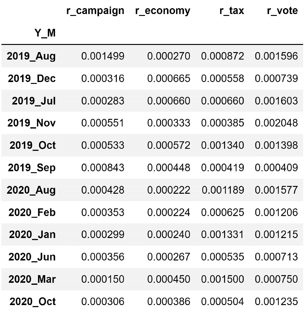
Figure 10.4 – vis_df

Now that we have vis_df, all that remains is to represent the information in vis_df in the form of a bar chart. The following subsection shows how this is done.

The last step – drawing the visualization

Figure 10.4 and Figure 10.1 are essentially presenting the same information. While Figure 10.4 (vis_df) uses a table to present the information, Figure 10.1 used a bar chart. In other words, we have almost made it and we need to perform one more step to create the requested visualization.

The following code block shows the code that creates the visualization shown in Figure 10.1. Pay attention before running the following code as you must import the matplotlib.pyplot module first. You can use import matplotlib.pyplot as plt to do this:

column_order = vis_df.sum().sort_values(ascending=False).index

row_order = speech_df.sort_values('Date').Y_M.unique()

vis_df[column_order].loc[row_order].plot.bar(figsize=(10,4))

plt.legend(['vote','tax','campaign','economy'],ncol=2)

plt.xlabel('Year_Month')

plt.ylabel('Average Word Frequency')

plt.show()

The preceding code creates two lists: column_order and row_order. As their names suggest, these lists are the order in which the columns and rows will be shown on the visual. The column_order is the list of words based on the summation of their occurrence ratio, while row_order is the list of Y_M based on their natural order in the calendar.

In this example, we learned about different techniques for level II data cleaning; we learned how to unpack columns and reformulate the data for the analytics tools and goals. The next example will cover data preprocessing to restructure the dataset.

What's the difference between restructuring and reformulating a dataset? We tend to use reformulate when the definition of data objects needs to change for the new dataset. In contrast, we use restructure when the table structure does not support our analytic goals or tools, and we have to use alternative structures such as a dictionary. In this example, we change the definition of a data object from one Donald Trump speech to Donald Trump's speeches in a month so we called this a dataset reformulation.

Here, we are being introduced to the new materials while immersing ourselves in examples. In this example, we learned about unpacking columns and reformulating the table. In the next example, we will be exposed to a situation that requires restructuring the table.

Example 2 – restructuring the table

In this example, we will use the Customer Churn.csv dataset. This dataset contains the records of 3,150 customers of a telecommunication company. The rows are described by demographic columns such as gender and age, and activity columns such as the distinct number of calls in 9 months. The dataset also specifies whether each customer was churned or not 3 months after the 9 months of collecting the activity data of the customers. Customer churning, from a telecommunication company's point of view, means the customer stops using the company's services and receives the services from the company's competition.

We would like to use box plots to compare the two populations of churning customers and non-churning customers for the following activity columns: Call Failure, Subscription Length, Seconds of Use, Frequency of use, Frequency of SMS, and Distinct Called Numbers.

Let's start by reading the Customer Churn.csv file into the customer_df DataFrame. The following screenshot shows this step:

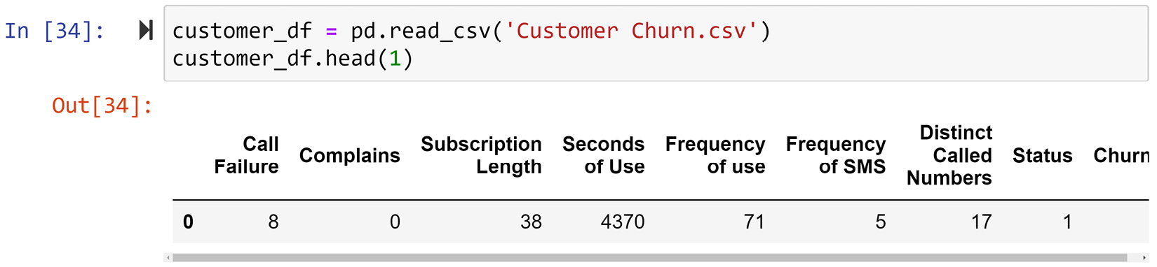
Figure 10.5 – customer_df before level I cleaning

At first glance, we can see that this dataset needs some level I data cleaning. While the column titles are intuitive, they can become more codable. The following line of code makes sure that the columns are also codable:

customer_df.columns = ['Call_Failure', 'Complains', 'Subscription_Length', 'Seconds_of_Use', 'Frequency_of_use', 'Frequency_of_SMS', 'Distinct_Called_Numbers', 'Status', 'Churn']

Before you move on, make sure that you study the new state of customer_df after running the preceding code.

Now that the dataset has been level I cleaned, we can pay attention to level II data cleaning.

This example needs us to draw six box plots. Let's focus on the first box plot; the rest will follow the same data cleaning process.

Let's focus on creating multiple box plots that compare the Call_Failure attribute of churning customers with that of non-churning customers. A box plot is an analytic tool that needs a simpler data structure than a dataset. A box plot only needs a dictionary.

What is the difference between a dataset and a dictionary? A dataset is a table that contains rows that are described by columns. As described in Chapter 3, Data – What is it Really?, in the The most universal data structure – a table section, we specified that the glue of a table is the definition of the data objects that each row represents. Each column also describes the rows. On the other hand, a dictionary is a simpler data structure where values are associated with a unique key.

For the box plot we want to draw, the dictionary we need has two keys – churn and non-churn – one for each population that will be presented. The value for each key is the collection of Call_Failure records for each population. Pay attention to the fact that, unlike a table data structure that has two dimensions (rows and columns), a dictionary only has one dimension.

The following code shows the usage of a pandas Series as a dictionary to prepare the data for the box plot. In this code, box_sr is a pandas Series that has two keys called 0 and 1, with 0 being non-churn and 1 being churn. The code uses a loop and Boolean masking to filter the churning and non-churning data objects and record them in box_sr:

churn_possibilities = customer_df.Churn.unique()

box_sr = pd.Series('',index = churn_possibilities)

for poss in churn_possibilities:

    BM = customer_df.Churn == poss

    box_sr[poss] = customer_df[BM].Call_Failure.values

Before moving on, execute print(box_sr) and study its output. Pay attention to the simplicity of the data structure compared to the data's initial structure.

Now that we have restructured the data for the analytic tool we want to use, the data is ready to be used for visualization. The following code uses plt.boxplot() to visualize the data we have prepared in box_sr. Don't forget to import matplotlib.pyplot as plt before running the following code:

plt.boxplot(box_sr,vert=False)

plt.yticks([1,2],['Not Churn','Churn'])

plt.show()

If the preceding code runs successfully, your computer will show multiple box plots that compare the two populations.

So far, we have drawn a box plot that compares Call_Failure for churning and non-churning populations. Now, let's create some code that can do the same process and visualizations for all of the requested columns to compare the populations. As we mentioned previously, these columns are Call_Failure, Subscription_Length, Seconds_of_Use, Frequency_of_use, Frequency_of_SMS, and Distinct_Called_Numbers.

The following code uses a loop and plt.subplot() to organize the six required visuals for this analytic so that they're next to one another. Figure 10.6 shows the output of the code. The data restructuring that's required to draw the box plot happens for each box plot shown in Figure 10.6. As practice, try to spot them in the following code and study them. I recommend that you review Chapter 1, Review of the Core Modules – NumPy and pandas, and Chapter 2, Review of Another Core Module – Matplotlib, if you don't know what the enumerate(), plt.subplot(), and plt.tight_layout() functions are:

select_columns = ['Call_Failure', 'Subscription_Length', 'Seconds_of_Use', 'Frequency_of_use', 'Frequency_of_SMS', 'Distinct_Called_Numbers']

churn_possibilities = customer_df.Churn.unique()

plt.figure(figsize=(15,5))

for i,sc in enumerate(select_columns):

    for poss in churn_possibilities:

        BM = customer_df.Churn == poss

        box_sr[poss] = customer_df[BM][sc].values

    plt.subplot(2,3,i+1)

    plt.boxplot(box_sr,vert=False)

    plt.yticks([1,2],['Not Churn','Churn'])

    plt.title(sc)

plt.tight_layout()

plt.show()

The following diagram is what you will get once the preceding code has been successfully executed:

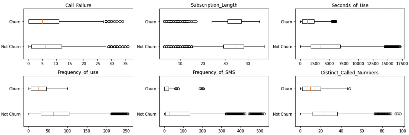
Figure 10.6 – End solution for Example 2 – restructuring the table

In this example, we looked at a situation where we needed to restructure the data so that it was ready for the analytic tool of our choice, the box plot. In the next example, we will look at a more complicated situation where we will need to perform both dataset reformulation and restructuring to make predictions.

Example 3 – level I and II data cleaning

In this example, we want to use Electric_Production.csv to make predictions. We are specifically interested in being able to predict what the monthly electricity demand will be 1 month from now. This 1-month gap is designed in the prediction model so that the predictions that come from the model will have decision-making values; that is, the decision-makers will have time to react to the predicted value.

We would like to use linear regression to perform this prediction. The independent and dependent attributes for this prediction are shown in the following diagram:

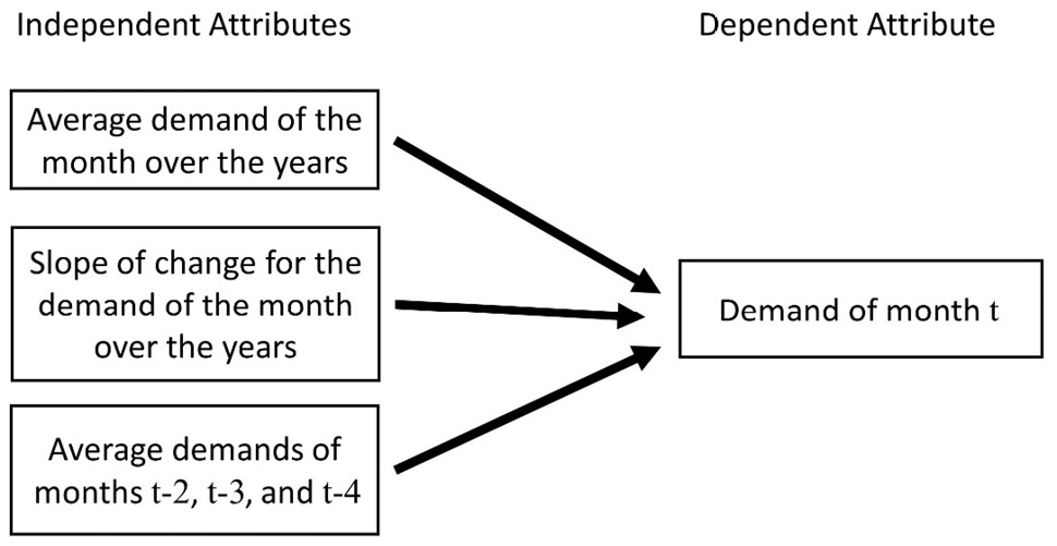
Figure 10.7 – The independent and dependent attributes needed for the prediction task

Let's go through the independent attributes shown in the preceding diagram:

• Average demand of the month over the years: For instance, if the month we want to predict demands for is March 2022, we want to use the average of the demands for every March in the previous years. So, we will collate the historical demands of March from the beginning of the data collection process (1985) to 2021 and calculate its average. This is shown in the following diagram.
• Slope of change for the demand of the month over the years: For instance, if the month we want to predict demands for is March 2022, we want to use the slope of change in the demand in March over the years. As shown in the following diagram, we can fit a line on the Demand in March data points across the years. The slope of that fitted line will be used for prediction.
• Average demands of months t-2, t-3, and t-4: In the preceding diagram, the t, t-2, t-3, and t-4 notations are used to create a time reference. This time reference is that if we want to predict the demand of a month, we want to use the average demand of the following data points: the monthly demand of 2 months ago, the monthly demand of 3 months ago, and the monthly demand of 4 months ago. For instance, if we want to predict the monthly demand of March 2021, we'd want to calculate the average of January 2021, December 2020, and November 2020. Note that we skipped February 2021 as it was our planned decision-making gap.
  

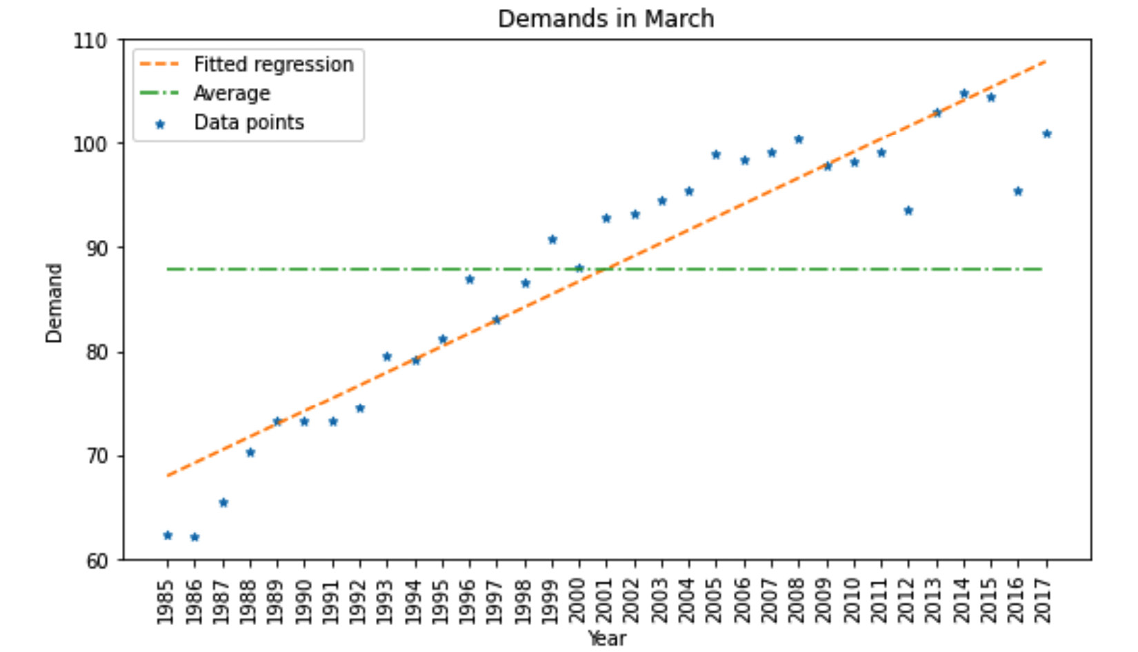
Figure 10.8 – Example of extracting the first two independent attributes for March

Now that we have a clear understanding of the data analytic goal, we will focus on preprocessing the data. Let's start by reading the data and covering its level I data cleaning process. The following screenshot shows the code that reads the Electric_Production.csv file into month_df and shows its first five and last five rows:

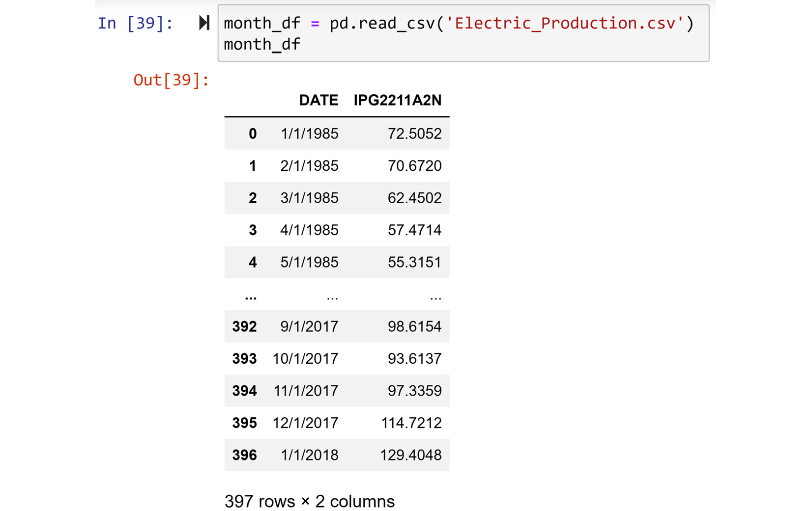
Figure 10.9 – month_df before level I data cleaning

At first glance, you can see that month_df can use some level I data cleaning. Let's get started.

Level I cleaning

The month_df dataset could do with the following level I data cleaning steps:

• The title of the second column can be more intuitive.
• The data type of the DATE column can be switched to datetime so that we can take advantage of datetime programming properties.
• The default index that's been assigned to the data by pandas can be improved as the DATE column would provide a better and more unique identification.

The following code takes care of the aforementioned level I data cleaning properties:

month_df.columns = ['Date','Demand']

month_df.set_index(pd.to_datetime(month_df.Date,format='%m/%d/%Y'),inplace=True)

month_df.drop(columns=['Date'],inplace=True)

Print month_df and study its new state.

Next, we will learn what level II data cleaning we need to perform.

Level II cleaning

Looking at Figure 10.7 and Figure 10.9 may give you the impression that the prescribed prediction model in Figure 10.7 is not possible as the dataset that's shown in Figure 10.9 only has one column, while the prediction model needs four attributes. This is both a correct and incorrect observation. While it is a correct observation that the data has only one value column, the suggested independent attributes in Figure 10.7 can be driven from month_df by some column unpacking and restructuring. That is the level II data cleaning that we need to do.

We will start by structuring a DataFrame that we want to restructure the current table into. The following code creates predict_df, which is the table structure that we will need for the prescribed prediction task:

attributes_dic={'IA1':'Average demand of the month', 'IA2':'Slope of change for the demand of the month', 'IA3': 'Average demands of months t-2, t-3 and t-4', 'DA': 'Demand of month t'}

predict_df = pd.DataFrame(index=month_df.iloc[24:].index, columns= attributes_dic.keys())

When creating the new table structure, predict_dt, the code is drafted while taking the following into consideration:

• The preceding code uses the attributes_dic dictionary to create intuitive and concise columns that are also codable. As predict_df needs to include rather long attribute titles, as shown in Figure 10.7, the dictionary allows the title columns to be concise, intuitive, and codable, and at the same time, you will have access to the title's longer versions through attributes_dic. This is a form of level I data cleaning, as shown in Chapter 9, Data Cleaning Level I – Cleaning Up the Table, in the Example 3 – intuitive but long column titles section. However, since we are the ones creating this new table, why not start with a level I cleaned table structure?
• The table structure we have created, predict_df, uses the indices of month_df, but not all of them. It uses all of them except for the first 24 rows, as specified in the code by month_df.iloc[24:].index. Why are the first 24 indices not included? This is due to the second independent attribute: Slope of change for the demand of the month over the years. As the slope of demand change for each month will be needed for the described prediction model, we cannot have a meaningful slope value for the first 24 rows of month_df in predict_df. This is because we at least need two historical data points for each month to be able to calculate a slope for the second independent attribute.

The following diagram summarizes what we want to accomplish by level II data cleaning month_df. The DataFrame on the left shows the first and last five rows of month_df, while the DataFrame on the right shows the first and last five rows of predict_df. As you already know, predict_df is empty as we just created an empty table structure that supports the prediction task. The following diagram, in a nutshell, shows that we need to fill predict_df using the data of month_df:

Figure 10.10 – Summary of data cleaning level II for Example 3

We will complete the depicted data processing and fill out the columns in predict_df in the following order: DA, IA1, IA2, and IA3.

Filling out DA

This is the simplest column filling process. We just need to specify the correct portion of month_df.Demand to be placed under predict_df.DA. The following screenshot shows the code and its impact on predict_df:

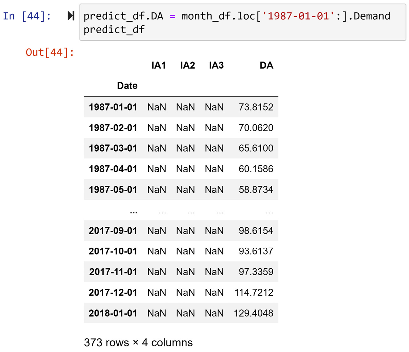
Figure 10.11 – Code for filling out predict_df.DA and its result

As we can see, predict_df.DA was filled out properly. Next, we will fill out predict_df.IA1.

Filling out IA1

To compute IA1, which is the Average demand of the month over the years, we need to be able to filter month_df using the value of the month. To create such a capability, the following code maps a lambda function to month_df and extracts the month of each row:

month_df['Month'] = list(map(lambda v:v.month, month_df.index))

Before you move on, print out month_df and study its new state.

The following code creates the ComputeIA1() function, which uses month_df to filter out the data points needed for the correct value of each cell under predict_df.IA1. Once it's been created, the ComputeIA1() function is applied to predict_df:

def ComputeIA1(r):

    row_date = r.name

    wdf = month_df.loc[:row_date].iloc[:-1]

    BM = wdf.Month == row_date.month

    return wdf[BM].Demand.mean()

predict_df.IA1 = predict_df.apply(ComputeIA1,axis=1)

The function ComputeIA1() that is written to be applied to the rows of predict_df, performs the following steps:

1. First, it filters out month_df using the calculated row_date to remove the data points whose dates are after row_date.
2. Second, the function uses a Boolean mask to keep the data points with the same month as the row's month (row_date.month).
3. Next, the function calculates the average demand of the filtered data points and then returns it.

   Note

   Let me share a side note before moving on. The wdf variable that was created in the preceding code is short for Working DataFrame. The abbreviation wdf is what I use every time I need a DataFrame inside a loop or a function but where I won't need it afterward.

After successfully running the preceding code, make sure that you print out predict_df and study its new state before moving on.

So far, we have filled out DA and IA1. Next, we will fill out IA2.

Filling out IA2

To fill out IA2, we will follow the same general steps that we did for filling out IA1. The difference is that the function we will create and apply to predict_df to calculate the IA2 values is more complex; for IA1, we created and applied ComputeIA1(), while for IA2, we will create and apply ComputeIA2(). The difference is that ComputeIA2() is more complex.

The code that creates and applies the ComputeIA2() function is shown here. Try to study the code and figure out how it works before moving on:

from sklearn.linear_model import LinearRegression

def ComputeIA2(r):

    row_date = r.name

    wdf = month_df.loc[:row_date].iloc[:-1]

    BM = wdf.Month == row_date.month

    wdf = wdf[BM]

    wdf.reset_index(drop=True,inplace=True)

    wdf.drop(columns = ['Month'],inplace=True)

    wdf['integer'] = range(len(wdf))

    wdf['ones'] = 1

    lm = LinearRegression()

    lm.fit(wdf.drop(columns=['Demand']), wdf.Demand)

    return lm.coef_[0]

predict_df.IA2 = predict_df.apply(ComputeIA2,axis=1)

The preceding code is both similar and different to the code we used to fill out IA1. It is similar since both ComputeIA1() and ComputeIA2() start by filtering out month_df to get to a DataFrame that only includes the data objects that are needed to compute the value. You may notice that the three lines of code under def ComputeIA1(r): and def ComputeIA2(r): are the same. The difference between the two starts from there. As computing IA1 was a simple matter of calculating the mean of a list of values, the rest of ComputeIA1() was very simple. However, for ComputeIA2(), the code needs to fit a linear regression to the filtered data points so that it can calculate the slope of the change over the years. The ComputeIA2() function uses LinearRegression from sklearn.linear_model to find the fitted regression equation and then return the calculated coefficient of the model.

After successfully running the preceding code, make sure that you print out predict_df and study its new state before moving on.

To understand the way ComputeIA2() finds the slope of change for each cell under predict_df.IA2, see the following screenshot, which shows the code and its output for calculating the slope for one cell under predict_df.IA2. The following screenshot calculates the IA2 value for the row with an index of 2017-10-01:

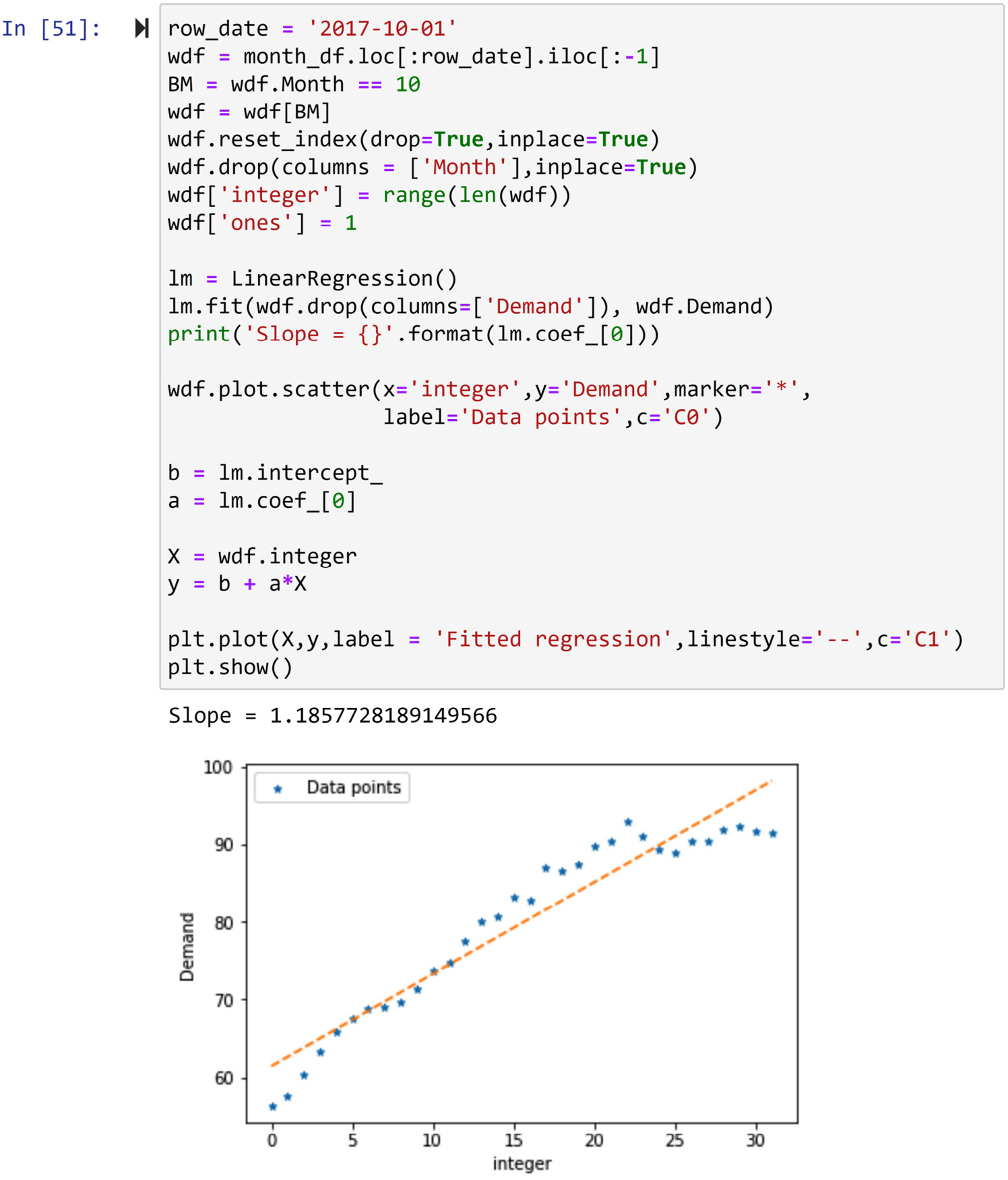
Figure 10.12 – A sample calculation of the slope (IA2) for one row of predict_df

So far, we have filled out DA, IA1, and IA2. Next, we will fill out IA3.

Filling out IA3

Among all the independent attributes, IA3 is the easiest one to process. IA3 is the Average demands of months t-2, t-3, and t-4. The following code creates the ComputeIA3() function and applies it to predict_df. This function uses the index of predict_df to find the demand values from 2 months ago, 3 months ago, and 4 months ago. It does this by filtering out all the data that is after row_date using .loc[:row_date], and then by only keeping the fourth, third, and second rows of the remaining data from the bottom using .iloc[-5:-2]. Once the data filtering process is complete, the average of three demand values is returned:

def ComputeIA3(r):

    row_date = r.name

    wdf = month_df.loc[:row_date].iloc[-5:-2]

    return wdf.Demand.mean()

predict_df.IA3 = predict_df.apply(ComputeIA3,axis=1)

Once the preceding code has been run successfully, we will be done performing level II data cleaning on month_df. The following screenshot shows the state of predict_df after the steps we took to create and clean it:

Figure 10.13 – Level II cleaned predict_df

Now that the dataset is level II cleaned and has been prepared for the prediction, we can use any prediction algorithm to predict the future monthly demands. In the next section, we'll apply linear regression to create a prediction tool.

Doing the analytics – using linear regression to create a predictive model

First, we will import LinearRegression from sklearn.linear_model to fit the data to a regression equation. As we learned in Chapter 6, Prediction to apply prediction algorithms to our data, we need to separate the data into independent and dependent attributes. Customarily, we use X to denote independent attributes and y to denote the dependent attribute. The following code performs these steps and feeds the data into the model:

from sklearn.linear_model import LinearRegression

X = predict_df.drop(columns=['DA'])

y = predict_df.DA

lm = LinearRegression()

lm.fit(X,y)

As we learned in Chapter 6, Prediction, once the preceding code has been executed, almost nothing happens, but the analysis has been performed. We can use lm to access the estimated βs and also perform prediction.

The following code extracts the βs from lm:

print('intercept (b0) ', lm.intercept_)

coef_names = ['b1','b2','b3']

print(pd.DataFrame({'Predictor': X.columns,                    'coefficient Name':coef_names,                    'coefficient Value': lm.coef_}))

Using the output of the preceding code, we can figure out the following regression equation:

To find out the quality of the prediction model, we can see how well the model has been able to find the patterns in the dependent attribute, DA. The following screenshot shows the code that draws the actual and fitted data of the linear regression model:

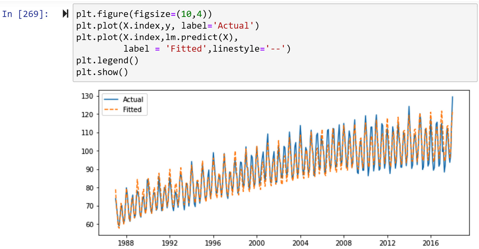
Figure 10.14 – Comparing the actual and predicted values of predict_df using linear regression

From the preceding diagram, we can see that the model has been able to capture the trends in the data very well and that it is a great model to be used to predict future data points.

Before moving on, take a moment to consider all we did to design and implement an effective predictive model. Most of the steps we took were data preprocessing steps rather than analytics ones. As you can see, being able to perform effective data preprocessing will take you a long way in becoming more successful at data analytics.

Summary

Congratulations on your excellent progress. In this chapter and through three examples, we were able to use the programming and analytics skills that we have developed throughout this book to effectively preprocess example datasets and meet the example's analytics goals.

In the next chapter, we will focus on level III data cleaning. This level of data cleaning is the toughest data cleaning level as it requires an even deeper understanding of the analytic goals of data preprocessing.

Before moving on and starting your journey regarding level III data cleaning, spend some time on the following exercises and solidify what you've learned.

Exercises

1. This question is about the difference between dataset reformulation and dataset restructuring. Answer the following questions:

   a) In your own words, describe the difference between dataset reformulation and dataset restructuring.

   b) In Example 3 of this chapter, we moved the data from month_df to predict_df. The text described the level II data cleaning for both table reformulation and table restructuring. Which of the two occurred? Is it possible that the distinction we provided for the difference between table restructuring and reformulation cannot specify which one happened? Would that matter?

2. For this exercise, we will be using LaqnData.csv, which can be found on the London Air website (https://www.londonair.org.uk/LondonAir/Default.aspx) and includes the hourly readings of five air particles (NO, NO2, NOX, PM2.5, and PM10) from a specific site. Perform the following steps for this dataset:

   a) Read the dataset into air_df using pandas.

   b) Use the .unique() function to identify the columns that only have one possible value and then remove them from air_df.

   c) Unpack the readingDateTime column into two new columns called Date and time. This can be done in different ways. The following are some clues about the three approaches you must take to perform this unpacking:

   • Use air_df.apply().
   • Use air_df.readingDateTime.str.split(' ',expand=true).
   • Use pd.to_datetime().

   d) Use what you learned in this chapter to create the following visual. Each line in each of the five line plots represents 1 day's reading for the plot's relevant air particle:

   

   Figure 10.15 – air_df summary

   e) Label and describe the data cleaning steps you performed in this exercise. For example, did you have to reformulate a new dataset to draw the visualization? Specify which level of data cleaning each of the steps performed.

3. In this exercise, we will be using stock_index.csv. This file contains hourly data for the Nasdaq, S&P, and Dow Jones stock indices from November 7, 2019, until June 10th, 2021. Each row of data represents an hour of the trading day, and each row is described by the opening value, the closing value, and the volume for each of the three stock indices. The opening value is the value of the index at the beginning of the hour, the closing value is the value of the index at the end of the hour, and the volume is the amount of trading that happened in that hour.

   In this exercise, we would like to perform a clustering analysis to understand how many different types of trading days we experienced during 2020. Using the following attributes, which can be found in stock_df.csv, we'd like to use K-Means to cluster the stock trading days of 2020 into four clusters:

   a) nasdaqChPe: Nasdaq change percentage over the trading day.

   b) nasdaqToVo: Total Nasdaq trading volume over the trading day.

   c) dowChPe: Dow Jones change percentage over the trading day.

   d) dowToVo: Total Dow Jones trading volume over the trading day.

   e) sNpChPe: S&P change percentage over the trading day.

   f) sNpToVo: Total S&P trading volume over the trading day.

   g) N_daysMarketClose: The number of days before the market closes for the weekend; for Mondays, it is 5, for Tuesdays, it is 4, for Wednesdays, it is 3, for Thursdays, it is 2, and for Fridays, it is 0.

   Make sure that you finish the clustering analysis by performing a centroid analysis via a heatmap and give each cluster a name. Once the clustering analysis is complete, label and describe the data cleaning steps you performed in this exercise.