Chapter 4: Databases

Databases play a major technological role in data preprocessing and data analytics. However, time and again, I have seen plenty of misunderstandings surrounding their role in analytics. While it is possible to do simple analytics and data preprocessing using databases themselves, these tasks are not what databases are designed for. In contrast, databases are technological solutions to record and retrieve data effectively and efficiently.

In this chapter, we will first discuss the technological role of databases in effective analytics and preprocessing. We will then enumerate and understand the different types of databases. Finally, we will cover five different methods of connecting to, and pulling data from, databases.

The following topics will be covered in this chapter:

• What is a database?
• Types of databases
• Connecting to, and pulling data from, databases

Technical requirements

You will be able to find all of the code and the dataset that is used in this book in a GitHub repository exclusively created for this book. To find the repository, click on this link, https://github.com/PacktPublishing/Hands-On-Data-Preprocessing-in-Python, find chapter 04 in this repository, and download the code and the data for better learning.

What is a database?

There may be a handful of different definitions of a database, all of which might be correct, but there is one definition that best serves the purpose of data analytics. A database is a technological solution to store and retrieve data both effectively and efficiently.

While it is true that databases are the technological foundations of data analytics, effective analytics do not happen inside them and that is a great thing. We want databases to be good at what they are meant to do: the effective and efficient storage and retrieval of data. We want a database to be fast, accurate, and secure. We also want a database to be able to serve our needs as regards quick sharing and synching.

When we want to get some data from databases for analytics purposes, it is easy to forget that databases are not designed to serve our analytics purposes. So, it should not be a surprise that the data in the database is organized in a way that serves its functions – the effective and efficient storage and retrieval of data – rather than being organized for our analytics purposes.

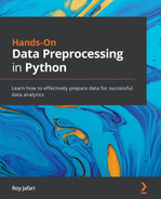
One of the very first steps of data analytics is to locate and collect data from various databases and sources, and reorganize it into a dataset that has the potential to answer questions about our decision-making environment. The following diagram illustrates this important step of data analytics:

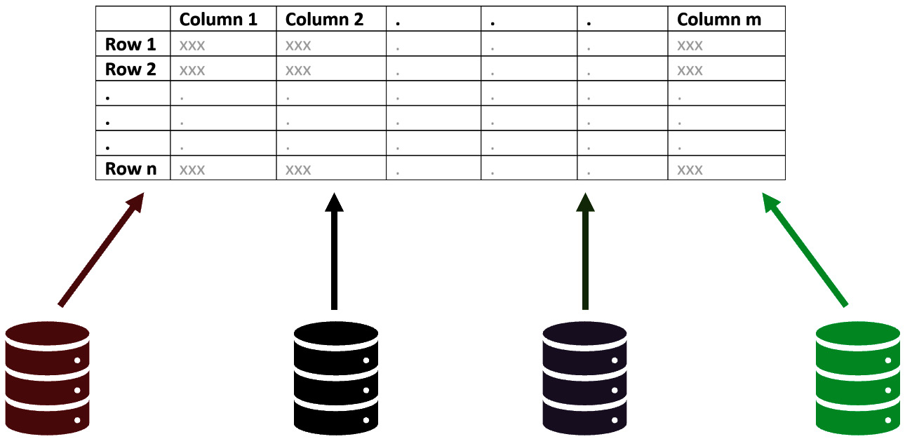
Figure 4.1 – From databases to a dataset

At times, the data might be coming from one database but, all the same, the data needs to be reorganized into a dataset that is designed for our analytics needs. When we are reorganizing the data into a dataset, we need to pay close attention to the dataset's definition of the data objects. We define the data object of a dataset so that the dataset serves the needs of our analytics.

Understanding the difference between a database and a dataset

A database and dataset are not the same concepts, but are often and incorrectly used interchangeably. We did define a database as a technological solution for storing and retrieving data both effectively and efficiently. However, a dataset is a specific organization and presentation of some data for a specific reason.

For data analytics, while the data comes from databases, it is eventually reorganized into a dataset. The "specific reason" for such a dataset is the analytics goals and the "specific organization and presentation" of that dataset is to support those goals.

For instance, we want to use weather data such as temperature, humidity, and wind speed to predict the hourly electricity consumption of the city of Redlands. For such analytics, we need a dataset whose definition of the data object is an hour in the city of Redlands. The attributes will be average temperature, average humidity, average wind speed, and electricity consumption. Pay attention that all of these attributes describe the data object – an hour in the city of Redlands. That is the design of the dataset that supports the analytical goal of predicting hourly electricity consumption in the city of Redlands based on weather data.

In the city of Redlands, the weather data and electricity data come from different databases. The weather data comes from 5 databases that collect data from 5 locations across the city, and each database records the weather data of its surroundings every 15 minutes. The electricity data comes from the city's only electricity supplier and its database records the amount of electricity consumption in the city every 5 minutes.

The data in these six databases needs to be collated and reorganized into the described dataset so that the prediction of hourly electricity consumption based on weather is possible.

Types of databases

Mainly there are four types of databases:

• Relational databases (or SQL databases)
• Unstructured databases (NoSQL)
• Distributed databases
• Blockchain

The distinctions between these databases are not cut and dried technologically and in practice. For instance, distributed databases are essentially a combination of different types of databases in multiple locations. Here, we will discuss these types of databases to develop a better appreciation for the way databases organize data according to a situation's needs. We will also briefly talk about the differences and similarities, as well as the advantages and disadvantages, of the types of databases.

Why do we need to know the types of databases for data preprocessing?

Each of the four types of databases organizes and stores the data differently. As our data analytics journey always involves locating and collecting data from various databases, knowing different kinds of databases serves two important purposes.

First, by knowing what is possible, we may be able to envision what could be out there when we look for data.

Second, and more importantly, as we want to reorganize the relevant data into our designed dataset, we need to understand the organization and structure of its source first.

The differentiating elements of databases

Before discussing the four types of databases, let's first talk about what are the elements that may require using various kinds of databases. These elements are the level of structure, storage location, and authority.

Level of data structure

Data with no structure is a pile of signs and symbols with no use or meaning. So do not let the term "unstructured databases" fool you since every piece of usable data needs at least some structure. The more data is structured, the less processing it will need when using it. However, structuring data is expensive and not always sensible.

When data is structured, not only does it potentially take up more space, but it also needs resources to preprocess and handle data before it is recorded. On the other hand, when the data is sufficiently structured on one occasion, it can then be used again and again. So, the way to determine how much structure data needs is to factor in the costs and benefits of structuring.

For example, while the benefits of structuring the basic customer data that is the core asset of many businesses easily outweigh its costs, in many cases, the costs of structuring customer emails, voice, and social media data may seem too overwhelming for small and medium organizations.

The following diagram shows the interaction between costs and benefits of structuring data. As the data is more structured, naturally, the cost of structuring it goes up. But in return, the cost of having to deal daily with unstructured data goes down until the benefits of structuring the data plateau. By considering the costs and benefits, we can find the appropriate level of data structure.

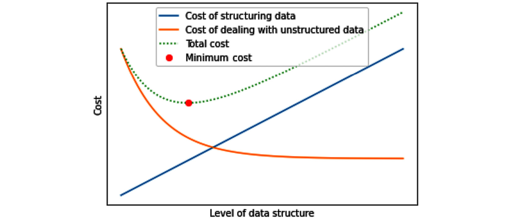
Figure 4.2 – Interaction between costs and benefits of structuring data – a general case

The best level of structuring data will vary from situation to situation and also from data to data. For instance, some data, such as video, sound, and social media data, may need specific preprocessing every time it is used for different purposes. That means every time it is used, it needs to go through data restructuring in any case, so structuring the data will not bestow any benefit and it does not make economical sense. Furthermore, these types of data tend to be large, and only a unique segment of them are needed to be structured from time to time without us not knowing which segment in advance. In such cases, structuring the whole data in advance does not make economical sense as we do not know what segment of the data we will need to be structured in the future. The following diagram shows this specific situation:

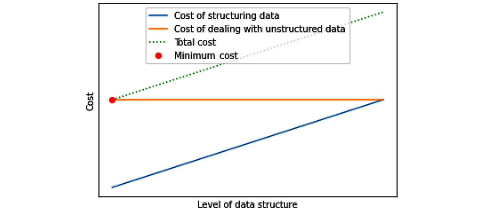
Figure 4.3 – Interaction between costs and benefits of structuring data – a specific situation

Storage location

The geographical location that the databases are located in is also important for a variety of reasons, including data security, data availability, data accessibility, and, of course, operation costs.

Authority

There are two key questions under authority that are very important to consider when choosing what type of database is appropriate:

1. Who does that data belong to?
2. Who should have the authority to update it?

Relational databases (SQL databases)

Relational databases, or structured databases, are an ecosystem of data collection and management in which both the collected data and the incoming data must conform with a pre-defined set of relationships between the data. For relational databases, if incoming data is not expected in a relational database, the data cannot be stored. Until the database ecosystem is updated in such ways, those types of incoming data are expected in the new ecosystem.

Some types of data are so different that updating the ecosystem of the database so that they are expected will only impede the database's goals. Furthermore, for some types of data, we may not be certain if we want to invest in them enough to change the ecosystem for them. This is often the case for video, voice, text, and social media data that tends to have a large size. For these types of data, we give up on changing the relational databases to accommodate them and store them in types of databases that do not require as much structuring.

Unstructured databases (NoSQL databases)

NoSQL, or unstructured databases, are precisely the solution for the problem of wanting to store data that we are unable to structure, or are ambivalent to do so. Furthermore, unstructured databases can be used as an interim house for data we do not have the resources to structure just now.

The term "unstructured databases" is not literal of course. Fully unstructured data is a pile of signs and symbols with no values. The term "unstructured databases" comes up against relational databases to create a distinction. The following example demonstrates a practical distinction between structured and unstructured data and their different applications for a law firm.

A practical example that requires a combination of both structured and unstructured databases

Seif and Associates law firm has been active in the area of civil and criminal law since 1956. Back in the day, the firm kept a paper copy of every legal document, every memo, every appeal, every invoice, and so on. In 1998, the firm went through a major IT overhaul and created a relational database that keeps track of all of the legal and business activities. The relational database that supports the firm is highly structured and allows the firm four different types of reports, that only such a highly structured database would allow. For instance, the database could report the monthly assigned legal tasks of every paralegal.

All of the documents that are sent out to the courts and the invoices that are sent to customers are not data objects in the database, but are produced on demand from the database. For instance, an invoice is produced every time by checking the invoice number in the database reading the items and prices associated with the invoice. Once all this data is found in the database, a piece of software puts them together and prints out an invoice every time.

As the major IT overhaul in 1998 was a significant undertaking by itself, the firm never had the chance to digitalize the paper copies from 1956 to 1998. However, 1 year ago, the firm decided to unburden itself from having to carry all those physical copies. Now, the firm keeps a scanned version of these documents on an unstructured database. Even though the data is all in the unstructured database, detailed reports from this database are not possible.

An AI company has recently approached the firm and suggested that they have the technology to go through the digital copies of the documents from 1956 to 1998 and include them in the structured database. The firm concluded that the cost of structuring that data (the AI company's price quote) does not meet or exceed the possible benefits of structuring it. Therefore, the firm decided that an unstructured database for those records will suffice as they are only recorded for legal purposes and if any of those documents are needed, the unstructured database has enough indexing, so the documents are found in 5 to 10 minutes.

Distributed databases

When we think of structured or unstructured databases, we normally assume that each database is located physically at one site or one computer. However, this can easily be an incorrect assumption. There are many reasons for having multiple locations/sites/computers for a database, such as higher data availability, lower operational costs, and superior data safety. Simply put, a distributed database is a collection of databases (structured, unstructured, or a combination of the two) whose data is physically stored in multiple locations. To the end user, however, it feels like just one database.

The foundation of cloud computing is distributed databases. For instance, Amazon Web Services (AWS) is a masterfully connected web of distributed databases across the world that offers database space with high availability and safety and bills its customers based on their actual usage.

Blockchain

We normally assume that a database is owned by one person or one organization. While this is a correct assumption in many cases, Blockchain is the solution when central ownership and authority are not advantageous.

For instance, this is one of the many reasons that Bitcoin has become a competitive option for digital money. While banks' central authority of the databases provides some assurances for data safety, the banks will also have the technological authority to cut customers off from their money if they deem this necessary. However, Blockchain is a database alternative that does not have a central authority while providing data safety.

The downside of Blockchain is that all of its data is stored in blocks and each block can only hold a small amount of information. Furthermore, the complex and detailed reports that are easily produced by relational databases cannot be created by Blockchain.

So far, we have covered some important topics:

• What are databases?
• Different types of databases
• Why we need various types of databases

Now, we turn our attention to how we can create and connect to databases and get the data we want.

Connecting to, and pulling data from, databases

For data analytics and data preprocessing, we need to have the skillset to connect to databases and pull the data we want from them. There are a few ways you can go about this. In this section, we will cover these ways, share their advantages and disadvantages, and, with the help of examples, we will see how this is done.

We will cover five methods of connecting to a database: direct connection, web page connection, API connection, request connection, and publicly shared.

Direct connection

When you are allowed access to a database directly, it means you can pull any data you want from the database. This is a great method of pulling data from databases, but there are two major disadvantages. First, you are rarely given direct access to databases unless you are completely trusted by the owner of the database. Second, you need to have the skillset to interact with a database to pull the data from it. The script you need to know for connecting to relational databases is called Structured Query Language (SQL). In SQL, every time you want to pull data from a database, you write a query using the SQL language. A great resource for learning SQL is available for free at W3Schools.com: https://www.w3schools.com/sql/.

Advice to beginners about learning SQL

If you are not familiar with SQL, make certain to at least know the following concepts: SQL table, primary keys, and foreign key, and the following operators: SELECT, DISTINCT, WHERE, AND, OR, ORDER BY, LIKE, JOIN, GROUP BY, COUNT(), MIN(), MAX(), AVE(), SUM(), HAVING, and CASE. https://www.w3schools.com/sql/ can help you learn the topics mentioned.

When you have written a correct query, you need to somehow send it to the database and be able to get back the results, and for that, you need a connection to the database. There is no one way to create a connection to the database. There is software with an interactive User Interface (UI) that can do that for you. Examples of such software are Microsoft Access, SQL Server Management Studio (SSMS), and SQLite.

The good news is that we can also create a connection to a database using the Python module sqlite3. We will be using the Chinook sample database to practice connecting to databases using Python and the module sqlite3. The following diagram shows the Chinook database using the Unified Modeling Language (UML). This sample database has 11 tables that are connected to one another by their primary keys to create a database that is designed to support a small/medium-sized business that sells music tracks. The UML of a database helps to understand the connections between tables and to design queries to pull data from a database.

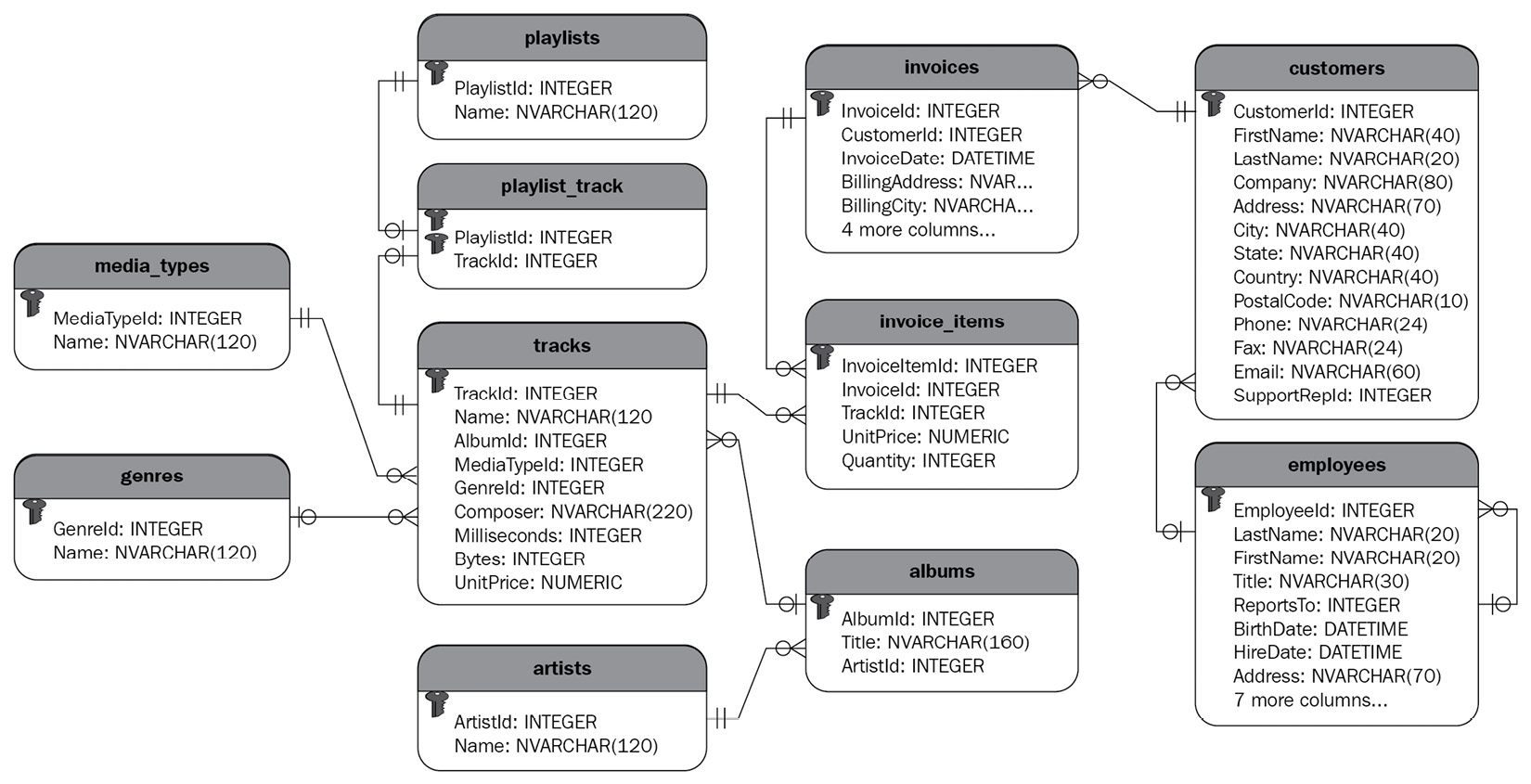
Figure 4.4 – UML of the Chinook database (source: sqlitetutorial.net)

The following screenshot shows the combined use of pandas and sqlite3 modules to create a connection to a database and read the data from the database into a pandas DataFrame. The code employs the function pd.read_sql_query() for this purpose. This function requires two inputs: a query in the form of a string and a connection. The code uses the sqlite3.connect() function to create a connection, and then passes Connection and query_txt into pd.read_sql_query() to have the requested data in a DataFrame.

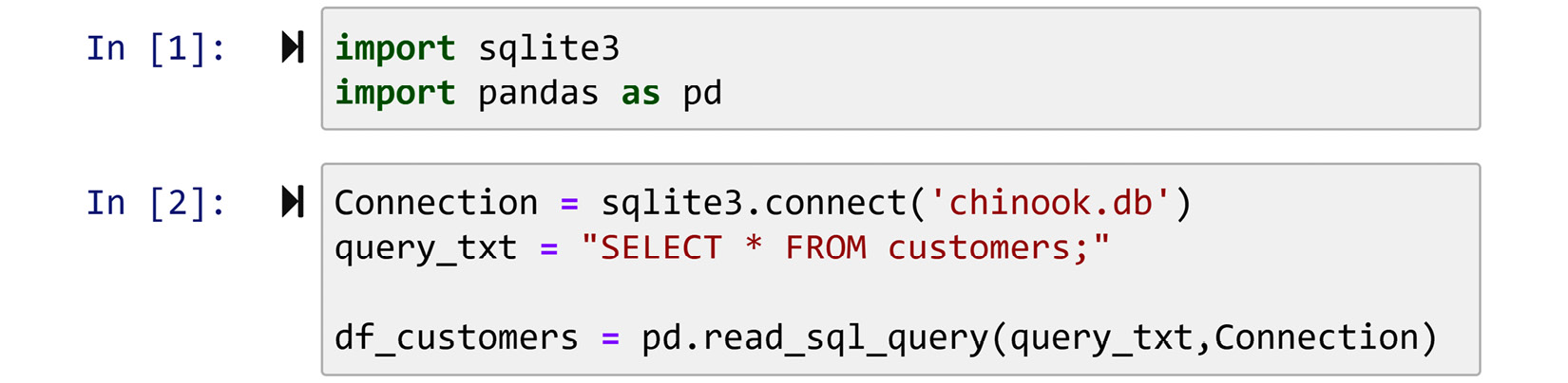
Figure 4.5 – Creating a connection to chinook.db using the sqlite3 module

So far, we have covered one of the five methods of connecting to databases: direct connection. Next, we will look at the four remaining methods: web page connection, API connection, request connection, and publicly shared.

Web page connection

Sometimes, the owner of the database only wishes to give you controlled access to their database. As these types of access are controlled, data sharing happens on the owner's terms. For instance, the owner might wish to give you access to a certain part of their database. Furthermore, the owner might not wish you to be able to pull all the data you need at once, but in timed portions.

A web page connection is one of the methods that database owners can use when offering controlled access to their database. A great example of a web page connection can be seen and interacted with at londonair.org.uk/london/asp/datadownload.asp. After you open this page, you can either pick a specific location or a specific measurement. Regardless of your choice, the page takes you to another page and takes more input from you before showing you a graph and providing you with a CSV dataset. Go to this web page and try different inputs and download some datasets before reading on.

API connection

The second method for giving out controlled access to databases is providing an API connection. However, unlike the web page connection method, where a web page would navigate and respond to your request, with API connections, a web server handles your data requests. A great example of data sharing through an API connection is data of the stock market. Different web services provide free and or subscription-based APIs for users to get access to live stock market data.

An example of connecting and pulling data using an API

The Finnhub Stock API (finnhub.io) is a great example of such a web service. Finnhub provides both free and subscription-based access to its databases. You can access and use their basic stock market data, such as daily, hourly, and minute by minute, of US stock prices. With their free version access, you can request their basic data, such as stock prices and you may send up to 60 requests per minute. If you need to process more than 60 requests per minute, or you want data that is not included in the free access, you will have to subscribe.

The Finnhub free version is enough for us to practice accessing data through APIs. First, on the first page of finnhub.io, click on Get a Free API Key and get yourself an API key. Second, type the following code into your Jupyter notebook and change API_Key from the arbitrary 'abcdefghijklmnopq' to the free API key you got from finnhub.io. If you have done every step correctly, you will get <Response [200]> printed out, which means everything went well. Via this code, you connected to the Finnhub web server and collected some data:

import requests

stk_ticker = 'AMZN'

data_resolution = 'W'

timestamp_from = 1577865600

timestamp_to = 1609315200

API_Key = 'abcdefghijklmnopq'

Address_template = 'https://finnhub.io/api/v1/stock/candle?symbol={}&resolution={}&from={}&to={}&token={}'

API_address = Address_template.format(stk_ticker, data_resolution, timestamp_from, timestamp_to, API_Key)

r = requests.get(API_address)

print(r)

Now, let's dissect this code together. Every API request needs to be expressed in a web address. This is universally true; the way you should translate your request into a web address might be somewhat different for different web servers, but they are very similar. If you have already run the proceeding code, when you execute print(API_address), as realized in the following screenshot, you will see the web address that claims to have the API key of abcdefghijklmnopq and requests the weekly Amazon stock price from January 1 to December 30, 2020. Study the web address and find out each segment of the address before reading on.

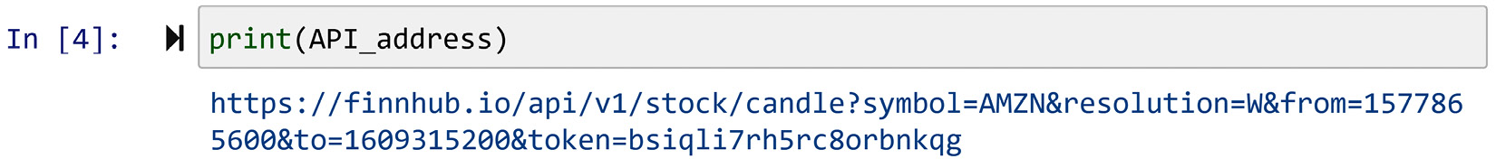
Figure 4.6 – Printing API_address

The following bullet points list and explain the different parts of the web address:

• symbol=AMZN specifies that you want the prices with the stock ticker AMZN, which indicates Amazon.
• resolution=W specifies that you want the weekly prices. You could request minute by minute, every 5 minutes, every 15 minutes, every half an hour, hourly, daily, weekly, and monthly prices by using, respectively, 1, 5, 15, 30, 60, D, W, and M.
• from=1577865600 specifies the time from which you want data. The weird-looking number is a timestamp for January 1, 2020.
• to=1609315200 specifies the time up to which you want data. The weird-looking number is a timestamp for December 30, 2020.
• token=abcdefghijklmnopq specifies the API key for this address.

What is next?

Now that you understand the preceding code and you have got the <Response [200]> message, we need to access and use the data. Let's do this step by step. First, run and study the output of the following code:

print(r.json())

The output is a JSON formatted string that has the following structure: {'c': a list with 51 numbers, 'h': a list with 51 numbers, 'l': a list with 51 numbers, 'o': a list with 51 numbers, 's': 'okay', 't: a list with 51 numbers, 'v': a list with 51 numbers}.

The output basically shows the 51-week data of Amazon stock prices. The following list shows what each letter stands for.

• 'c': the closing price for the period
• 'h': the highest price during the period
• 'l': the lowest price during the period
• 'o': the opening price for the period
• 's': the status of the stock
• 't': the timestamp showing the end of the period
• 'v': the trading volume in the period

Working with the stock data when presented with this format is not easy. However, transforming it to a format that you are used to is easy. Run the following code and study the output:

AMZN_df = pd.DataFrame(r.json())

AMZN_df

After running the code, the data will be presented in AMZN_df, which is a pandas DataFrame. A pandas DataFrame is a data structure that we like as we know how to manipulate the data using multiple pandas functions.

Putting it all together

The following screenshot shows all the preceding code that created AMZN_df and another six lines of code that are added to restructure the data into a more presentable and codeable format:

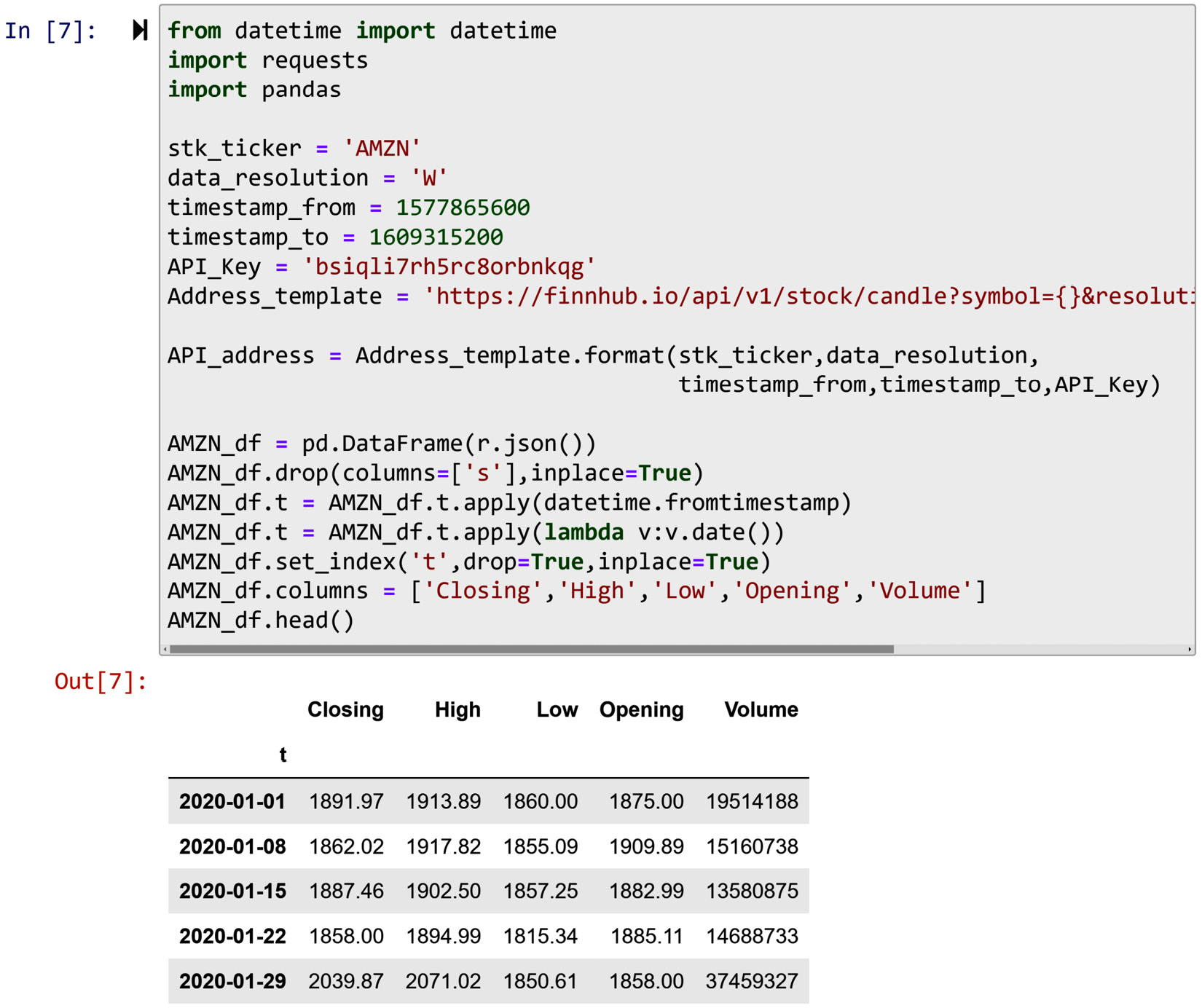
Figure 4.7 – An example of using an API connection to connect and pull data

The following list indicates how each added line of code contributes to this goal.

• inplace=True: When this is added to a pandas function, you mean to specify that you want the requested change to be applied to the DataFrame itself. The alternative is to have the function output a new DataFrame that has the requested change. This code is added to two of the following lines of code.
• AMZN_df.drop(columns=['s'],inplace=True): This line of code drops the column s as this column only has one value across all the data objects.
• AMZN_df.t = AMZN_df.t.apply(datetime.fromtimestamp): This line of code applies the datetime.fromtimestamp function from the datatime module to the column t. This function takes a timestamp and transforms it into a DateTime object. Run datetime.fromtimestamp(1609315200) to see the workings of this function.
• AMZN_df.t = AMZN_df.t.apply(lambda v:v.date()): This line of code applies a lambda function to only keep the date part of a DataTime object as the time for all the data objects is 16:00.
• AMZN_df.set_index('t',drop=True,inplace=True): This line of code sets the column t as the index of the DataFrame. The part drop=True indicates that you want the original index to be dropped.
• AMZN_df.columns = ['Closing','High','Low','Opening','Volume']: This line of code changes the name of AMZN_df columns.
• AMZN_df.head(): This line of code outputs a DataFrame with only the first five rows of the AMZN_df DataFrame.

So far, we have covered three of the five methods of connecting to databases: direct connection, web page connection, and API connection. Next, we will look at the remaining two methods: request connection and publicly shared.

Request connection

This type of connection to a database happens when you do not have any access to the database of interest under any of the three preceding methods, but you know someone who has access and is authorized to share some parts of the data with you. In this method, you need to clearly explain what data you need from the database. This method of accessing the database has some pros and cons. See Exercise 4 to figure out what they are.

Publicly shared

This method of connecting to databases is the least flexible. Under the publicly shared method, the owner of the database has extracted one dataset out of the databases they owned and has provided access to that one dataset. For instance, almost all of the datasets that you find on kaggle.com fall under this method of connecting to a database. Furthermore, most of the data access that is provided under data.gov also falls under this inflexible access to the databases.

Summary

Congratulations on successfully finishing this chapter! Now you are equipped with a powerful understanding of databases and it will pay dividends in your quest for effective data preprocessing.

In this chapter, you learned the technological role of databases in data analytics and data preprocessing. You also learned about different kinds of databases and how they should be chosen for different situations. Specifically, you understood how you would decide about the level of data structures in their databases. Last but not least, you learned the five different methods of connecting to, and pulling data from, databases.

This chapter concludes your learning of part 1 of this book: Technical needs. Now you are ready to start learning about analytics goals, which is the second part of this book. The technical needs will empower you to use technology to effectively read and manipulate data. The analytics goals will give you a foundational understanding so that you know for what purposes you will need to manipulate the data.

The next part of the book will be an exciting one as we will see examples of what can be done with data. However, before moving on to the next part, take some time and solidify and improve your learnings by completing the following exercises.

Exercises

1. In your own words, describe the difference between a dataset and a database.
2. What are the advantages and disadvantages of structuring data for a relational database? Mention at least two advantages and two disadvantages. Use examples to elucidate.
3. In this chapter, we were introduced to four different types of databases: relational databases, unstructured databases, distributed databases, and Blockchain.

   a. Use the following table to specify a ranking for each of the four types of databases based on the criteria presented in the table.

   b. Provide reasoning for your selections.

   The table already has some of the rankings to get you started. N/A stands for Not applicable. Study the ranking provided and give your reasoning as to why they are correct.

   

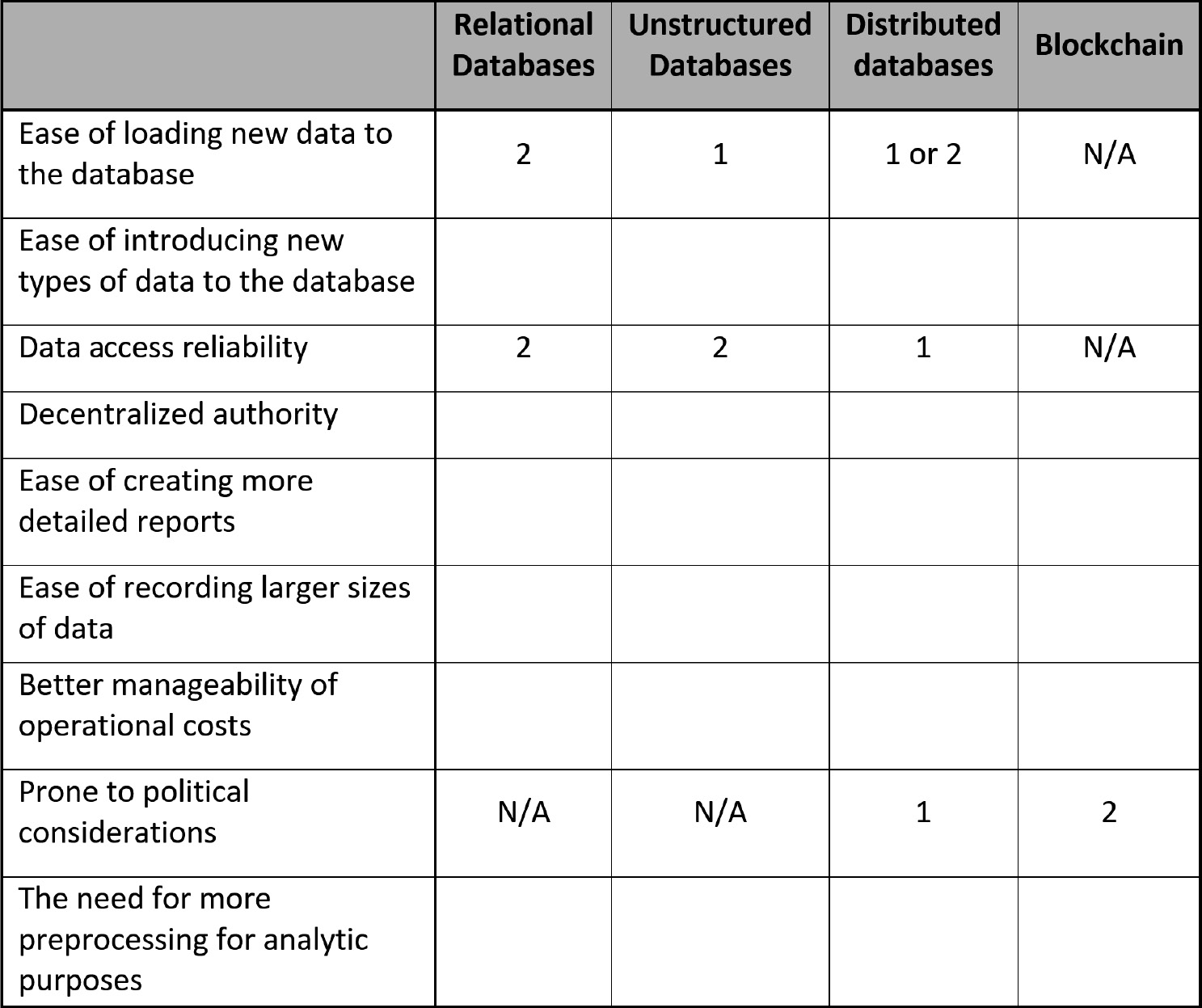
   Figure 4.8 – Database type ranking

4. In this chapter, we were introduced to five different methods for connecting to databases: direct connection, web page connection, API connection, request connection, and publicly shared. Use the following table to indicate a ranking for each of the five methods of connecting to databases based on the specified criteria. Study the rankings and provide reasoning as to why they are correct.
   

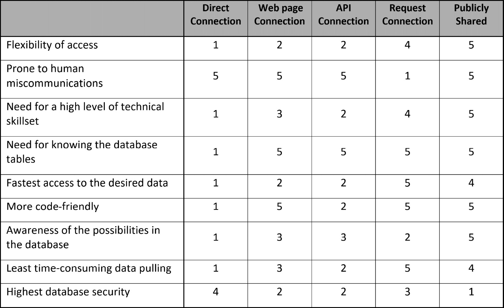
   Figure 4.9 – Ranking of database connection methods

5. Using the Chinook database as an example, we want to investigate and find an answer to the following question: Do tracks that are titled using positive words sell better on average than tracks that are titled with negative words. We would like to focus solely on the following words in the investigations:

   List of negative words: ['Evil', 'Night', 'Problem', 'Sorrow', 'Dead', 'Curse', 'Venom', 'Pain', 'Lonely', 'Beast']

   List of positive words: ['Amazing', 'Angel', 'Perfect', 'Sunshine', 'Home', 'Live', 'Friends']

   a. Connect to the Chinook database using Sqlite3 and execute the following query:

   SELECT * FROM tracks join invoice_items on tracks.TrackId = invoice_items.TrackId

   b. Use the skills you learned in previous chapters (applying a function, group by function, and so on) to come up with a table that lists the average total sales for tracks containing good words and the same for tracks containing bad words. Here is what the table will look like:

   

   Figure 4.10 – Table report from the Chinook database for Exercise 5

   c. Report your conclusions.

6. In the year 2020, which of the following 12 stocks experienced the highest growth.

   Stocks: ['Baba', 'NVR', 'AAPL', 'NFLX', 'FB', 'SBUX', 'NOW', 'AMZN', 'GOOGL', 'MSFT', 'FDX', and 'TSLA']

   For a good estimate of growth, use both formula 1 and formula 2 on the weekly closing stock prices. (a) Formula1: (a-b), and (b) Formula2: (a-b)/c

   In these formulas, a, b, and c are, respectively, the stock closing price for 2020, the median of stock prices during 2020, and the mean of stock prices during 2020.

   Based on each formula, what is the stock with the highest growth, and what is the difference between the outcome of each formula?