
15 Plunger Solenoids and Their Control
15.1 Introduction
Plunger solenoids are electromagnetic actuators with 1(2) dc- or ac-fed coils, without or with permanent magnets, with limited (from a few tens of mm to 10–20 mm) linear motion of a soft magnetic core (Figure 15.1a) or PM mover (plunger Figure 15.1b) via attraction or even repulsive electromagnetic forces. Plunger solenoids are also called electromagnets and are used extensively in standard applications such as electric power switches (relays), door lockers etc., enjoying substantial worldwide markets.
Reference [1] presents a classical study of electromagnets.
Essentially, for plunger solenoids, on–off supply control is used as the forward motion is secured by the electromagnetic force while the backward motion is done by the mechanical spring to save energy [2].
To avoid the bouncing of the plunger as travel ends, a more advanced supply (and control) has to be provided. Bouncing is detrimental to the fixture that meets the plunger, in the sense of wearing, and should be limited.
In some applications, where the extreme positions should be maintained without current in the coil(s)—zero latching losses—the PM force has to overcompensate the mechanical spring force (Figure 15.2) [3].
For controlled positioning (with or without mechanical spring), advanced power control is needed, because, in general, the open loop system is statically and dynamically unstable (without PMs and without a mechanical spring).
Magnetic suspension in MAGLEVs is a particular case of controlled position solenoids, but, due to the interference of vehicle motion and the multiple degrees of freedom motions, the latter’s design and control will be discussed in separate chapters. Also, in applications with constant frequency oscillatory linear motion, operation at resonance is sought to increase efficiency (and power factor) and thus reduce the power electronics kilovoltampere (kVA) ratings (and costs).
Linear oscillatory motors will thus be dealt with in a dedicated chapter.
Therefore, plunger solenoids treated here are restricted to nonoscillatory linear reciprocating motion when they close and open fluid flow (as in valve actuators) or electric current flow (as in electric contactors, etc.); also, small travel fast response is investigated with priority; position control will also be investigated for industrial small travel applications.
In view of the many topologies and applications, we will start here with the principles of PM-less plunger solenoids, then continue with their modeling, considering magnetic saturation and eddy currents; subsequently, a few design and control studies are developed in considerable detail, for configurations without and with PMs. Finally, a rather complete case study of FEM and dynamic modeling, optimal design, and position sensor-less control for PM twin-coil valve actuators is performed.
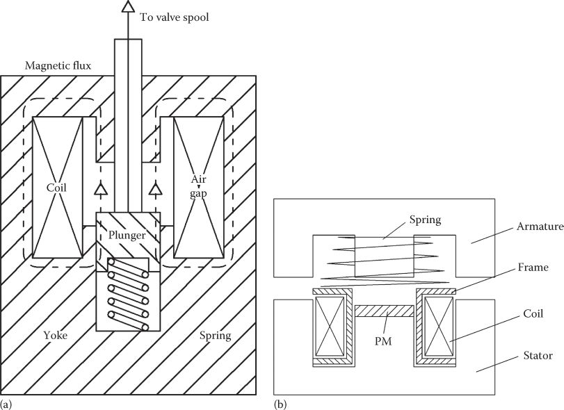
FIGURE 15.1 Cylindrical-shaped plunger solenoid: (a) without PM and (b) ac power switch with PMs in the stator.
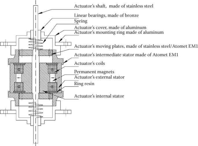
FIGURE 15.2 PM plunger solenoid with zero latching losses. (After Agarlită, S., Linear single phase PM oscillatory machine: Design and control, PhD thesis, UPT.ro, 2009.)
15.2 Principles
The PM-less plunger solenoids (Figure 15.1) include a cylindrical (in general) stator with a mild steel solid core or made of solid magnetic composite (SMC) with rather high permeability and small enough electrical conductivity (σel < 1.5 · 106 Ω−1m−1), a multiturn coil and an SMC mover (plunger).
When the coil is voltage supplied, the current starts increasing and the plunger moves against the spring force until it closes the airgap (a residual resin-filled airgap is practical to avoid stacking).
When the voltage is turned off, the mechanical spring increases the airgap rather quickly. So far, no control is implied.
The attraction force between the plunger and the stator core may be calculated based on stored magnetic energy Wmag or coenergy Wcomag:
with
where
ψ is the flux linkage
i is the current
The simple formulae (15.1) and (15.2) imply that no eddy currents are induced in the stator. In the absence of magnetic saturation, the dependence of total magnetic flux linkage of the coil flux linkage ψ on current i is linear and the slope depends on plunger position x (Figure 15.3).
The instantaneous force Fx is the same with both formulae in (15.1) and, for increased airgap x by Δx, the magnetic energy decreases while the coenergy increases (Figure 15.3) with airgap increase. Magnetic saturation produces a departure from the linearity of flux linkage ψ(x, i) curve family (Figure 15.3d).
The average mechanical work and force Fxav over an energy cycle, in the presence of magnetic saturation (Figure 15.3d), is proportional, at constant current operation, to the area AOABCD.
On the other hand, if the turn-off current coil energy is returned by power electronics to the source, its contribution is proportional to the area AOCBDO, when losses are considered zero. So the energy conversion ratio per energy cycle ηen is
Apparently, magnetic saturation increases the energy conversion ratio per energy cycle; unfortunately, it does not do this for the same average thrust, for the same device, and for the same airgap excursion length (from xmin to xmax). However, higher ηen means a better utilization of the power electronic supply because magnetic saturation reduces the transient inductance of the coil. Consequently, the current rising and decaying are faster; that is, faster response in current and thus in force is obtained.
We will continue with a linear lump circuit model of the plunger solenoids, still ignoring magnetic saturation and eddy currents.
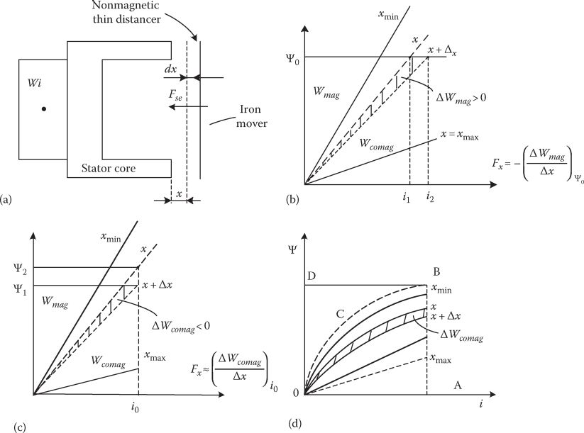
FIGURE 15.3 Instantaneous force from energy and coenergy differential (a) the basic topology of plunger solenoid; (b) constant flux magnetic energy increment ΔWmag; (c) constant current coenergy increment (μiron = ∞); (d) flux linkage/current/position curves family with magnetic saturation.
15.3 Linear Circuit Model
A more detailed geometry of the plunger solenoid is shown in Figure 15.4.
During dc voltage turn-on (or off), both the current i and the plunger position x vary (from l0 to l1 and vice versa).
The mechanical spring is supposed to bring back the mover at xmin = l0. The electric circuit equation is straightforward:
where
R is the coil resistance
Ll is the coil leakage inductance
Lm is the coil main inductance (airgap inductance when µiron = ∞)
For µiron = ∞, the main inductance Lm is approximately

FIGURE 15.4 Basic plunger solenoid with one mechanical spring, (a) and equilibrium zone, (b).
with
On the other hand, the motion equation can be written as
Equations 15.5 and 15.6 may be arranged into a state space format with either (ψ, x, dx/dt) or (i, x, dx/dt) as variables:
As evident from (15.7), due to electromagnetic force complex formula, even in the absence of magnetic saturation and eddy currents, the third-order solenoid state space model is nonlinear.
Its stability may be approached by linearization: feedback linearization [4], linearization around an equilibrium point [5], asymptotically exact linearization [6], etc.
Linearization around an equilibrium point is the standard procedure used to yield insights into the general behavior, while feedback linearization is preferred when a feedback control law that transforms the nonlinear plant model into a linear one is targeted.
As we will dwell on dynamics and control later in this chapter, it suffices to say at this stage that, as known from Earnshaw’s theorem, the plunger solenoid without a mechanical spring is statically and dynamically unstable, for constant voltage (or current) supply.

FIGURE 15.5 Current i and position x versus time for a solenoid-spring system, fed with constant dc voltage: (a) current and (b) displacement.
Static stabilization for particular displacement zones (X1 → X2 in Figure 15.5) may be obtained with an adequate spring and for a certain current (i = 2 A in Figure 15.5).
For larger current, the system is statically stable first at only one point (X3) and then it becomes statically unstable. In reality, the current is not constant for constant voltage supply. Solving the state space model (15.7) through numerical methods in time for M = 10 g, B = 0.0001 N s/m, R = 1 Ω, starting, W1 = 200 turns, A = 1 cm2, K = 100 N/m, l1 = 3 cm, the current and position versus time in Figure 15.5 are obtained.
After the motion starts, the current increases first but then, due to motion start, the emf increases and as the inductance also increases, the current decreases; when the motion ends (after 28 ms; inductance is large [small airgap]), the current increases slowly toward V0/R value, as expected. The results in Figure 15.5 are to be corrected by the influence of magnetic saturation and of eddy currents in the magnetic cores. During voltage turn-off, the skin effect in the cores delays the flux penetration and thus delays the occurrence of flux (force); magnetic saturation, fortunately, also reduces the inductance, increases the penetration depth, and thus has a “positive dynamic effect.” During voltage turn-on, the current may decay quickly to zero (especially if the supply may apply not a zero but a negative voltage or a varistor is placed in series).
But, due to eddy currents, the delay in magnetic flux decay occurs, and thus the attraction force decay is slower. This phenomenon delays the spring retraction motion. Consequently, it is imperative to investigate quantitatively the influence of eddy currents and magnetic saturation.
15.4 Eddy Currents and Magnetic Saturation
Flat active area solenoids may be made of laminations, though noise and vibration may be excessive, but for tubular topologies, which are notably more favorable (in terms of manufacturability), soft magnetic composite iron cores are the solution.
The cylindrical structure allows for approximate analytical eddy current solution, due to cylindrical symmetry, besides the use of FEM-transient methods.
We first investigate the eddy currents in a flat solid mild steel structure in order to grasp the essentials and then use a nonlinear circuit model with eddy currents for a quantitative thorough analysis of the plunger solenoid transients. The FEM inclusion of eddy currents is investigated later in the chapter for case studies of design and control.
For an infinite flat plate placed in the YX plane (Figure 15.6), a tangential uniform magnetic field H (along X), existing at time zero, is removed instantly.
The magnetic 1D eddy current field equation in iron is straightforward:
with σiron and μiron as electrical conductivity and magnetic permeability.
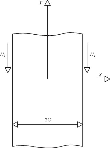
FIGURE 15.6 Flat solid iron plate.
Also,
and
By using the separation of variables for the Fourier series method, the solution of (15.8) is
The Fourier series converges quickly and thus, approximately, the average flux density Bav(t), for constant permeability, is
But, if magnetic saturation is not neglected, μiron should be replaced by (transient permeability):
Now the magnetization curve may be approximated by polynomials such as

FIGURE 15.7 Field penetration for step magnetic field (mmf) change.
Let us consider a1 = 295, b1 = 384, c1 = 178, a′1= 1, b′1 = 0.6, c′1 = 0.34 for a 10 mm thick plate (2c = 10 mm) with σi = 2.5 · 106 Ω−1 m−1, and use FEM, for constant and variable permeability, for sudden magnetic field (mmf) application and removal [7]—Figure 15.7.
For the linear (nonsaturated) case, left side in Figure 15.7, the field builds up in 255 ms, while for heavy saturation (Figure 15.7b), it takes only 7.5 ms. The field decay (Figure 15.7c) is slower for the saturated core and it takes 200 ms. To corroborate these FEM results with the analytical expression in (15.2), we may define a magnetic inductance of eddy currents Leddy, [8] besides the iron magnetic reluctance (resistance) Riron:
The corresponding time constant
Ap, lp are plate cross section and field path length, respectively.
But Tiron should be consistent with the time dependence in (15.12):
As a single value of permeability was considered in Riron and Leddy, its value does not appear in (15.17). In reality, to account approximately for local magnetic saturation variation during transients, both Riron and Leddy may be corrected [8] as
S is called severity factor, and linearization is performed for small flux variation around Φss. Notable improvements have been obtained this way, as seen in Figure 15.8 [8] for the example in Figure 15.7, for S = 66.4. Other eddy current delay considerations in the circuit model have been introduced with relative success [9,10].
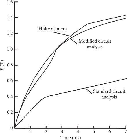
FIGURE 15.8 Transient response for a nonlinear flat plate to a 1592 A/m surface field. (After Caridies, J.P., Fast acting electromagnetic actuators, PhD thesis, Department of Mechanical Engineering, Pennsylvania State University, University Park, PA, 1982.)
Besides FEM—with eddy currents and magnetic saturation considered—the aforementioned nonlinear model may be used for optimal design and control system design in order to save precious computation time for reasonable relative precision.
15.5 Dynamic Nonlinear Magnetic and Electric Circuit Model
A more realistic circuit model of the plunger solenoid not only accounts for magnetic saturation and eddy currents but also for the leakage and airgap magnetic fluxes Φl, Φg. FEM field distribution for a C core solenoid suggests that we may separate the coil mmf into a first part (αwi), which is responsible for the leakage flux, and a second one ((1 − α)wi), which determines essentially the airgap (force producing) flux.
Making use of the magnetic reluctances and magnetic inductances of stator (Rs, Lls), mover (Rm, Llm) cores, of airgap Rg, the dynamic magnetic circuit in Figure 15.9 is obtained. The reluctance Rlm refers to the flux paths produced by the total mmf.
The dynamic circuit model equations are rather straightforward:
We add the voltage and motion equation, for completing the model:
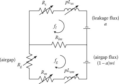
FIGURE 15.9 Dynamic magnetic circuit of plunger solenoid. (After Caridies, J.P., Fast acting electromagnetic actuators, PhD thesis, Department of Mechanical Engineering, Pennsylvania State University, University Park, PA, 1982.)
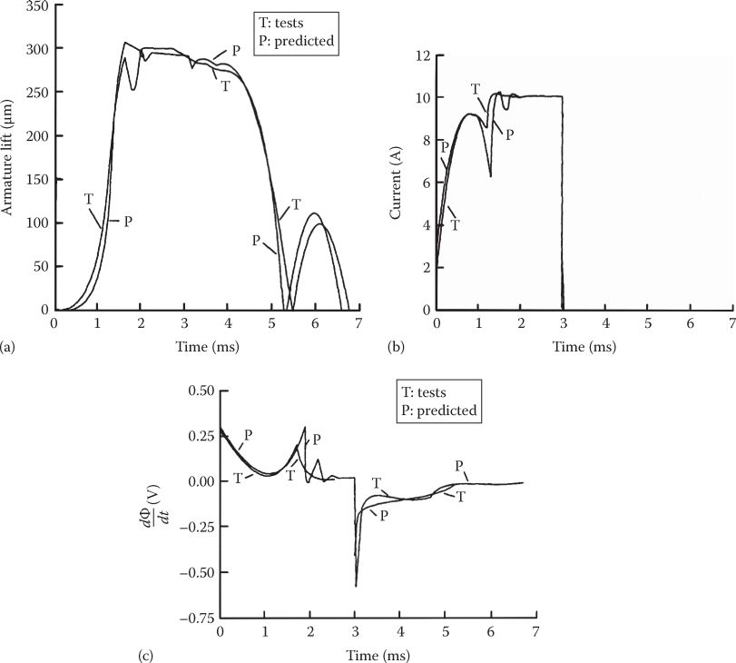
FIGURE 15.10 Dynamic transients: test versus predicted results: (a) position, (b) current, and (c) airgap flux time derivative. (After Caridies, J.P., Fast acting electromagnetic actuators, PhD thesis, Department of Mechanical Engineering, Pennsylvania State University, University Park, PA, 1982.)
In the attraction force expression (Fx in (15.22)), magnetic saturation has already been considered in calculating the airgap flux Φg, but it is ignored in the airgap magnetic reluctance Rg (which depends only on airgap).
Sample results obtained with this model [8] are shown in Figure 15.10.
In matching predicted to measured force versus displacement results, a residual airgap (of less than 20 μm) was added to account for contact surface imperfections; this may be necessary if a minimum nonmagnetic airgap coating is applied on contact surfaces.
Although the current decays quickly after voltage turn-off (Figure 15.10b), the plunger position takes reasonably more time until the first touchdown. In addition, in the absence of any control (or of strong damping), there is a notable plunger bouncing, which should be limited in order to prolong the life of the solenoid.
While the aforementioned analysis seems to establish the essentials of plunger solenoids, what follows describes a few implementations with their design and control issues for specific applications.
15.6 PM-Less Solenoid Design And Control
PM-less plunger solenoids are less expensive (due to the absence of PMs) and, provided with low-loss SMC cores, they may be used both in on–off motion applications (such as power relays, compressed-air valves) and in position controlled valves. They will be discussed next as they provide devices with smaller volume and faster response performance.
A typical compressed gas-valve plunger solenoid is shown in Figure 15.11 [11].
To get an idea of magnitudes, let us consider an airgap variation interval from 0.25 to 0.5 mm with an outer solenoid diameter of around 27 mm and a mover total weight of about 15 g; travel time of 0.25 mm is 0.5 ms.
The volume constraints lead to the chamfer (Figure 15.11) in the mover, with an angle of inclination α as object to optimization. An equivalent magnetic circuit may be built (as done in previous paragraphs); the attraction force is obtained both on the horizontal and on the inclined (chamfered) section on the mover.
The optimal chamfer angle (for maximum force) α ≈ 40°. For the coil design (height (b) and length (a)), through complex simulations, the acceleration time is calculated for already installed 10 A in the coil (Figure 15.12) [11].
The lowest acceleration time (tmin ≤ 0.5 ms) is obtained for b ≈ 20 mm and a ≈ 3.0 mm (250 turns/coil) with a mover of 15 g. The equivalent electric conductivity of the magnetic cores is σiron = 1.4 · 106 Ω−1 m−1.
The thrust versus airgap for 15 and 25 A and the coil current i(t) and the force Fx(t) are shown in Figure 15.13.
The control sets the magnitude and slope of the open-phase triggering and the magnitude and duration of the hold of open phase. There is some delay between current and force peak values. The eddy current phenomenon impedes the current (force) gradients. The considered core material (σiron = 1.41 · 106 Ω−1m−1) allows for a fast enough (less than 0.2 ms) magnetic field penetration time (as proved by the force/time gradient (Figure 15.13b)).
For the controlled position of a high-frequency band, a PM-less solenoid should act as push-pull, with two units [12], Figure 15.14.
The dual solenoid model may be used also for radial magnetic bearings control.
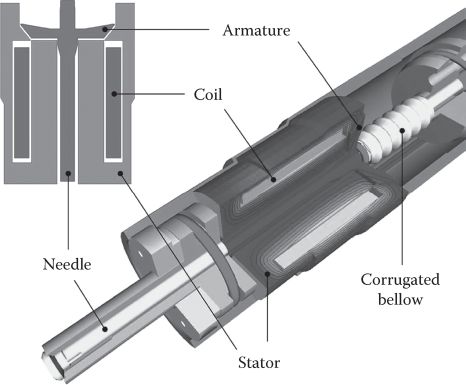
FIGURE 15.11 PM-less solenoid as on–off valve actuator. (After Albert, J. et al., IEEE Trans., MAG-45(3), 1741, 2009.)
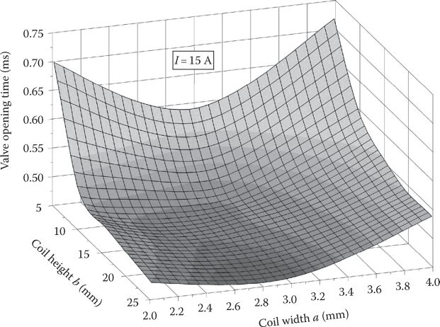
FIGURE 15.12 Opening time (for 0.25 mm travel) variation with coil length a and height b. (After Albert, J. et al., IEEE Trans., MAG-45(3), 1741, 2009.)
The dynamic model (with μiron = ct and no eddy currents) is rather straightforward (based on the linear model in Section 15.3):
An example for d = 3.85 · 10−3 m, β0 = 4.4 · 10−4 N m2/A2, R1 = R2 = 100 Ω, M = 0.015 kg, Fu = 18.5 N s/m, Fc = 1.3 N is illustrated here. The two coils are turned on in shifts (or, for faster response, differential control of the two solenoids by v1 = v0 + Δv, v2 = v0–Δv may be performed). For robust position control response of the nonlinear system of (15.23), quite a few strategies may be applied.
Gain scheduling [5] switching PI, on–off and zero vibration on–off control [12] (Figure 15.15), or sliding mode control [13] may be tried.
For zero vibration on-off control [12], overshooting and bouncing are not visible but the response quickness is not particularly high (tens of milliseconds).
15.6.1 Bouncing Reduction
Now in single solenoid on–off control, for opening classic valves (contacts), the plunger bouncing against the stator (valve) chair has to be attenuated. Even for a simplified control scheme (Figure 15.16) [14], bouncing reduction is possible without position feedback (or estimation) and without close-loop control.
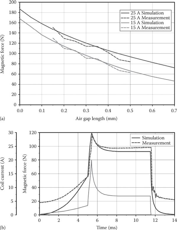
FIGURE 15.13 Calculated and measured: (a) force/airgap and (b) current and force versus displacement (for standard power amplifier supply). (After Albert, J. et al., IEEE Trans., MAG-45(3), 1741, 2009.)
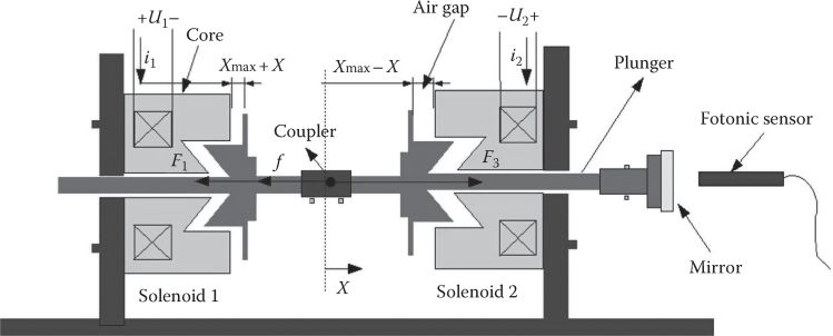
FIGURE 15.14 Dual PM-less solenoid. (After Yu, L. and Chang, T.N., IEEE Trans, IE-57(7), 2519, 2010. With permission.)
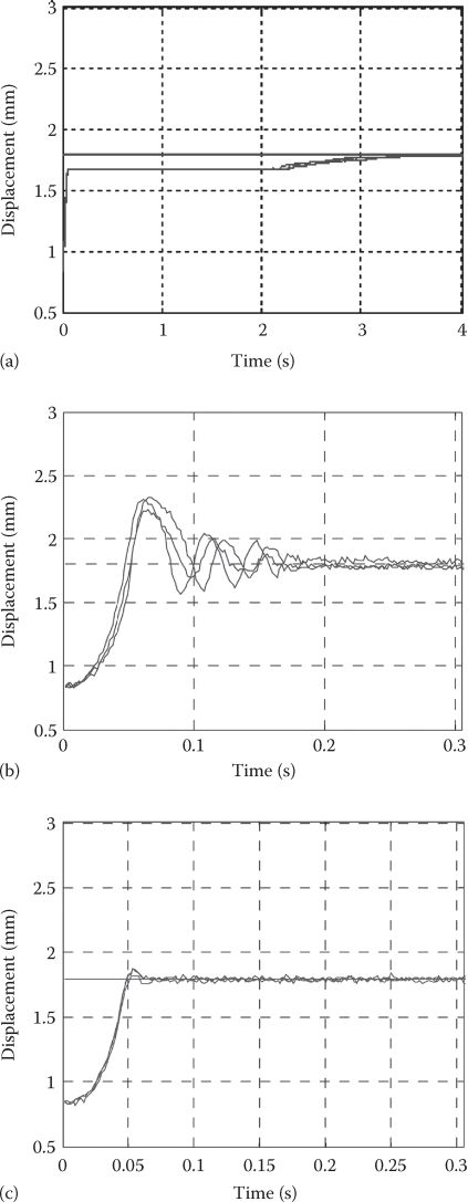
FIGURE 15.15 Experimental position step response: (a) with switching PI control, (b) with on-off control, and (c) with zero vibration on-off control (set point: 1.8 mm; initial point: 0.85 mm). (After Yu, L. and Chang, T.N., IEEE Trans, IE-57(7), 2519, 2010.)
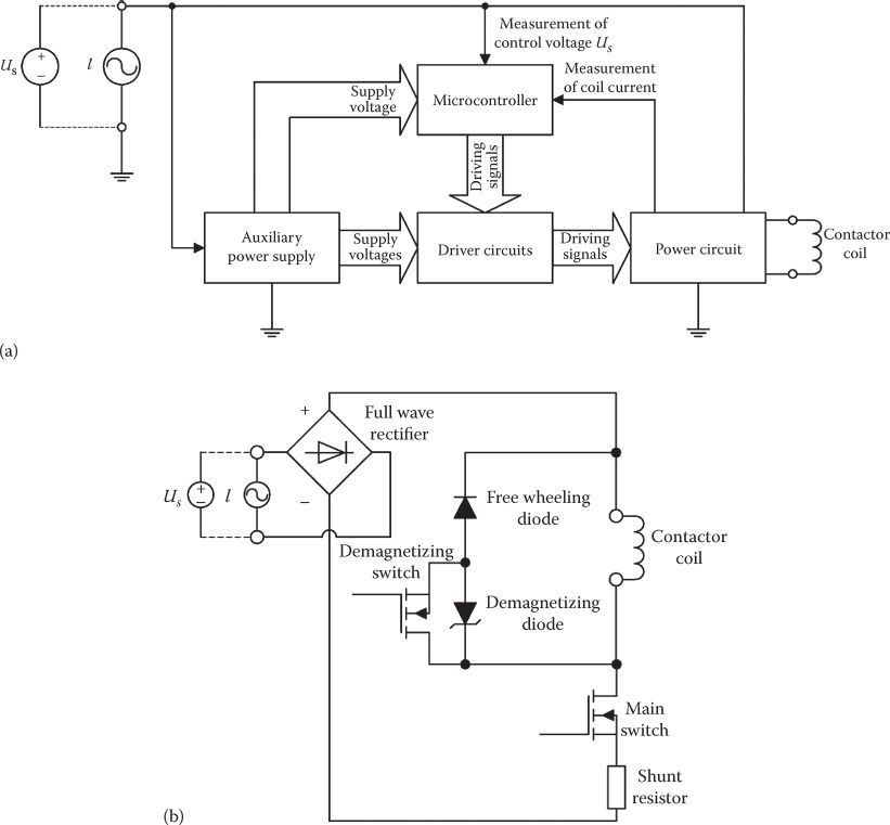
FIGURE 15.16 On-off solenoid control with bouncing reduction (a) and power supply (b). The dc power source (direct or with a diode rectifier) is controlled with a dc-dc converter that in turn, controls the coil current. (After de Morales, P.M.S.D. and Perin, A.J., IEEE Trans, IE-55(2), 861, 2008.)
The freewheeling diode, the demagnetization (Zener) diode, and the switch allow for fast current decay (reduction of the electric time constant by the Zener diode). The main power switch is off either when the current is too large or at the end of the turn-off period. A drop in the current profile occurs when the mover motion starts; consequently, a current first decay, below an experimentally learned threshold, indicates that the motion is about to end (the contactor closes). For an ac power source (without rectification), a more complicated detection through current profile is still feasible [14]. The holding current is further reduced to Ihold (also found by trial and error).
The bouncing reduction depends on the fast detection of mover motion and, consequently, on the validity of current samples (which should be ignored close to zero voltage crossing, to avoid large error).
This limitation suggests that, perhaps, reduced bouncing with faster motion (even position) detection (estimation) is the next solution for better performance.
15.6.2 FEM Direct Geometric Optimization Design
Quite a few FEM direct geometric optimization designs of PM-less solenoids have been introduced (such as level-set [15] or geometric algorithms [16]); as only a few geometrical variables are used for optimization, both magnetic saturation and eddy currents may be considered (Figure 15.17, after [16]).
15.7 Pm Plunger Solenoid
15.7.1 PM Shielding Solenoids
When no latching (at zero current) is required, the PM may be used for shielding—that is, for flux deviation—in order to produce higher force for the given geometry and mmf (losses) [17], Figure 15.18.
The PMs shielding and the stepped airgap lead to larger force and thus, for constant current, the force does not vary much with airgap (Figure 15.18b); this indicates favorable conditions for position close-loop control. The voltage-on and voltage-off transients (Figure 15.18c and d) are very similar to those in Figure 15.10, derived for PM-less plunger solenoids.
The flux ψ(t, x) and force F(t, x) variations are calculated by FEM [17]. The fast closing of the contact (Figure 15.18c) is achieved but, again, eddy currents delay the displacement decrease during voltage turn-off (Figure 15.18d), when the motion is determined mainly by the mechanical spring (K = 1700 N/m, mover mass 0.77 g!).
15.7.2 PM-Assisted Solenoid Power Breaker
Single (Figure 15.19a) and dual-coil (Figure 15.19b) PM solenoids [19] have been proposed for fast response power circuit breakers.
The main asset of PM assistance in plunger solenoids is to provide holding force at zero current, which leads to lower energy consumption, when the holding time is rather large in relative values.
Typical, practical control strategies for the single and dual coil PM solenoids are shown in Figure 15.20.
Loop I (Figure 15.20a) refers to “making loop” while loop II refers to the “breaking loop.” For ac voltage supply, the initial phase voltage may vary randomly; the initial angle of voltage has a strong influence on the displacement/time, which is, however, in the millisecond range (Figure 15.21a).
The dual coil PM solenoid (Figure 15.21b) [19] designed for a 3200 A/400 V circuit breaker shows 22 ms making time, 3 ms trigger time, and 13 ms breaking time (Ca = 10,000 μF, Cb = 1,000 μF). For PM solenoids, the PM holding force at travel end is larger than the mechanical spring force at one end for the single coil and at two ends for the dual coil.
Another dual coil PM solenoid for small excursion—submillimeter range (20–30 μm)—application was proposed for surface machining, micro-optics, metal molds, light-enhanced films, and axial active magnetic bearings [20]; accelerations up to 100 times the gravitational acceleration (forces of 100 N for a plunger mass of 12–15 g) are required.
While the force/volume capability of PM plunger solenoids in various high dynamics applications seems to be competitive, the optimization design and the better loss assessment and robust control are subjects of paramount importance in the effort to extend controlled PM solenoid markets.
For a more elaborate case study, we will investigate now a twin-coil (single inverter control) PM solenoid, intended for valve actuating, in terms of analytical, FEM, circuit model, optimization design, and close-loop sensorless control.
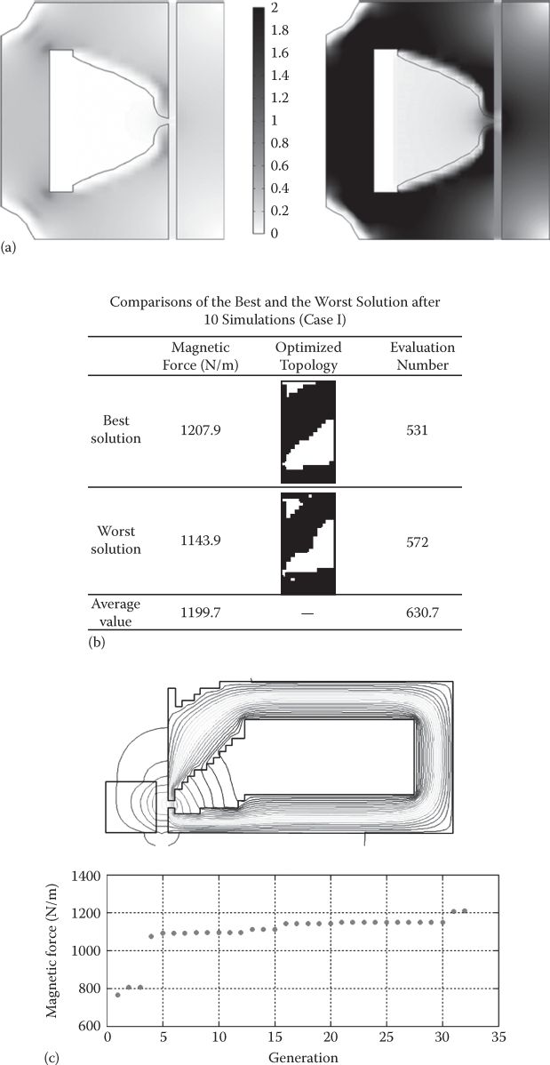
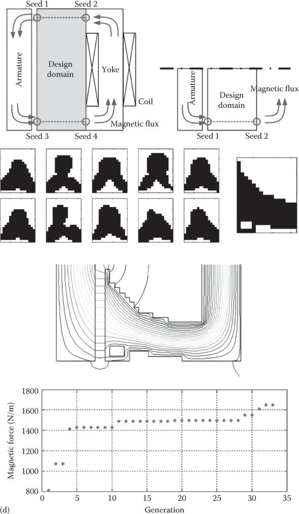
FIGURE 15.17 Optimal topology FEM design, (a), level-set method, (b). (After Park, S. and Min, S., IEEE Trans, MAG-46(2), 618, 2010.) (c) GA optimization. (d) GA optimization. (After Choi, J.S. and Yoo, J., IEEE Trans., MAG-45(5), 2276, 2009.)
15.8 Case Study: PM Twin-Coil Valve Actuators
15.8.1 Topology and Principle
The PM twin-coil valve actuator investigated here is shown in Figure 15.22.
The PM twin-coil actuator is controlled by a single inverter, and thus the twin-coil mmf produced magnetic field does not cross the PMs; consequently, the danger of demagnetization is reduced. In addition, the eddy currents induced in the PMs are reduced this way. There are some eddy currents produced by the PMs themselves as the magnetic field in the PMs varies a little with mover position; it will be shown that the division of the ring-shape PM into a few sectors drastically reduces the PM eddy currents.
The actuator is kept in both mover extreme positions by the PM (cogging) force, which has to surpass the mechanical spring force.
Although the frequency of motion varies widely for a car engine valve actuator, mechanical springs are provided to globally better exchange energy during the vehicle’s most used speed range. Changing the polarity of current in the twin coils changes the direction of total force and quickly drives the mover back and forth.
Using a single inverter is considered here a good asset in terms of initial system cost reduction.

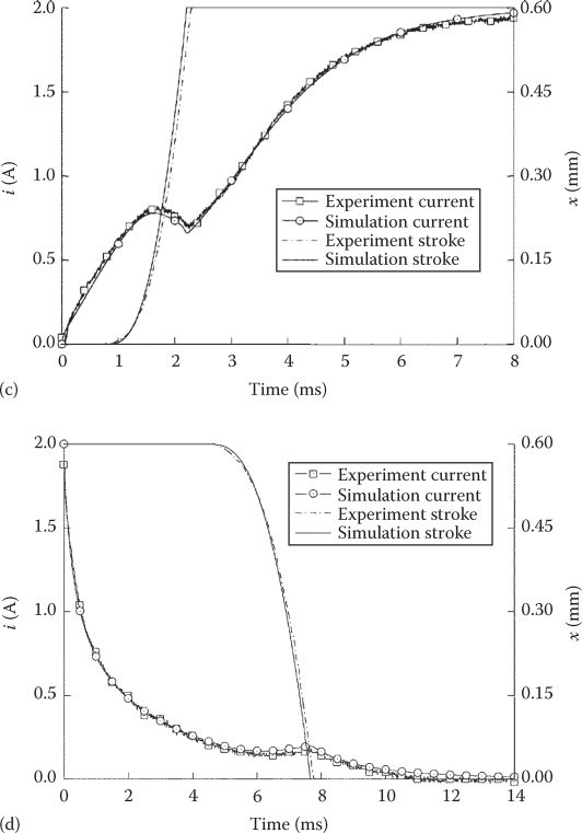
FIGURE 15.18 Tubular PM-shield plunger solenoid: (a) the topology, (b) force displacement. Tubular PM-shield plunger solenoid: (c) current and displacement versus time during contact closing, and (d) current and displacement versus time during contact opening. (After Man, J. et al., IEEE Trans, MAG-46(12), 4030, 2010.)
A variable valve car transmission needs essentially
Zero holding current
±4 mm travel, within 3–4 ms, enough for 6 krpm engine speed
Low (soft) landing velocity: less than 0.3 m/s at 6 krpm engine speed
Maximum valve speed: 3.5 m/s
Peak valve-mover acceleration: 5000 m/s2
Package (valve) volume ≤0.2 dm3
Up to 600 N developed thrust
No more than 3 kVA peak power for an 8 intake + 8 exhaust valve engine
Low electrical time constant to facilitate fast force dynamics
These are very demanding specifications unmet yet in industrial applications by plunger solenoid valve actuators (without or with PMs).
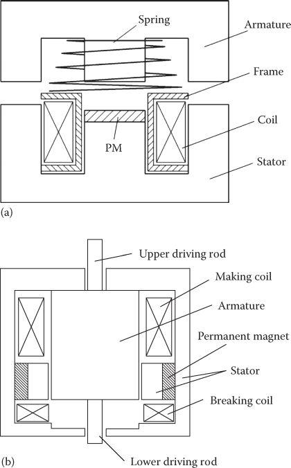
FIGURE 15.19 PM-assisted solenoid power breakers (a) with single coil and (b) with dual coil. (After Fuang, S., IEEE Trans., MAG-45(7), 2990, 2009.)
15.8.2 FEM Analysis
As the volume constraints are very challenging, magnetic saturation will be heavy, and thus only 2D FEM may produce practical useful results. The Atomet EM1 soft magnetic composite core losses will be computed after magnetostatic FEM field variation calculations.
They are proven to be modest in comparison with copper losses (Atomet M1 reaches 1.5 T at 20 kA/m), for the dimensions marked in Figure 15.23.
The FEM calculated PM cogging force, total force, total coil flux, and the transient inductance are given in Figure 15.24a through d.
The forces have been calculated using the weighted stress tensor volume integral.
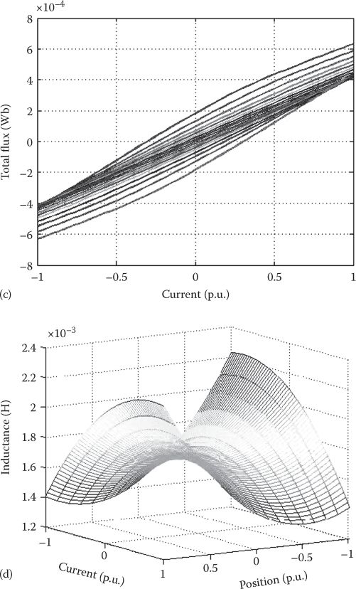
An acceptable agreement of measured and calculated forces is visible in Figure 15.24. Further on, the actuator cores have been divided into eight regions with different flux-density time variation patterns; then these ±Bmax variations were used to calculate the core losses here:
with ρA-EM1 = 7100 kg/m3, p100 Hz, 1 t = 20 W/kg.
Finally, adding different current values of all eight volume contributions, the results in Figure 15.25 are obtained.
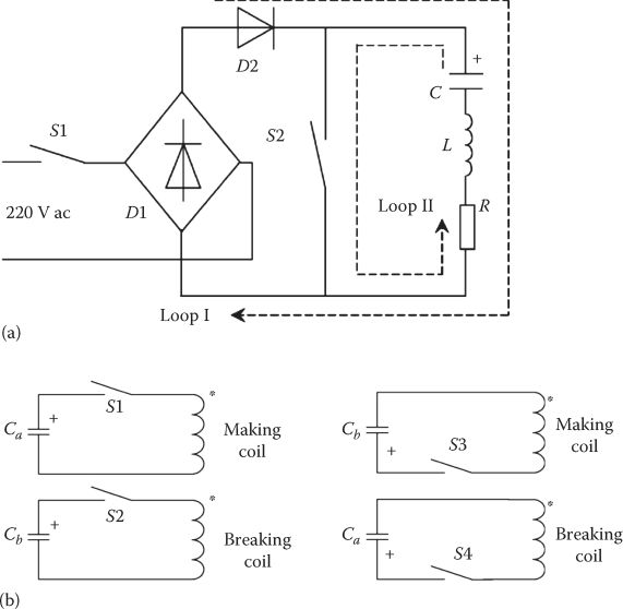
FIGURE 15.20 Control circuit system. (After Fuang, S. et al., IEEE Trans., MAG-45(10), 4566, 2009.) (a) single-coil PM solenoid and (b) dual coil PM solenoid (making and braking control).
It is notable that pcore < 1.6 W; if we add the 3 W PM eddy current losses (the ring-shaped PM is made of eight sectors), we get 4.6 W, which is rather small in comparison with 115 W copper losses at 21 A (RMS) sinusoidal current.
Thermal and mechanical FEM analyses have also been performed. The temperature evolution at maximum current is shown in Figure 15.26a; mechanical stress results are visible in Figure 15.26b.
While mechanically the stress distribution is within bounds, for a temperature-safe operation, SmCo5 PMs are to be used.
15.8.3 Direct Geometrical FEM Optimization Design
Grid search and three variations of Hooke-Jeeves optimization method have been used to optimize the design of PM twin-coil valve actuator.
First, the objective function and its constraints are placed:
FPmax > 300 N—PM force
Kf = Fmax/FP max > 1.8—force coefficient
amax ≥ 5000 m/s2 (maximum acceleration of the mover)
pcopper < 120 W—copper losses
Actuator volume: vol < 0.2 L
Now the variable vector is chosen: r0—shaft radius, r1—interior shaft average radius, r2—intermediate stator average radius, r3—external stator interior radius, r4—external stator external radius, lPM—PM height (axial), lk—axial air zone height between coils and stator core; lc—coil height (axial); lm—mover plate height (axial); h—intermediate stator external height.
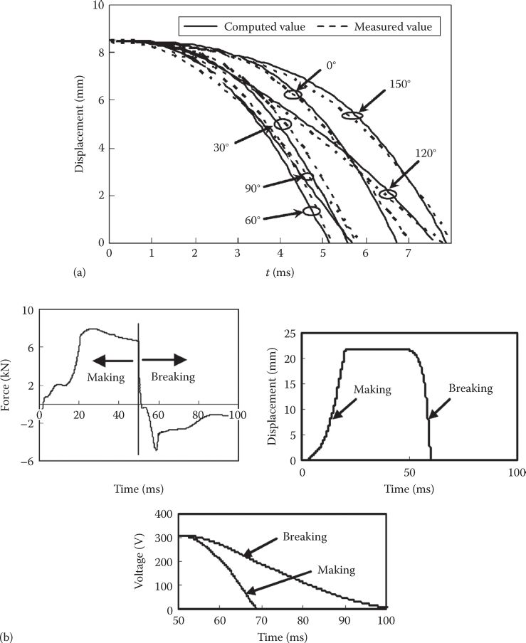
FIGURE 15.21 Displacement/time (single-coil PM solenoid), (a); force, displacement, voltage versus time, dual coil PM solenoid dynamics, (b). (After Fuang, S. et al., IEEE Trans., MAG-45(10), 4566, 2009.)
About 2300 situations have been run by the grid search method, with the best results as follows: FPM = 343.92 N, Fmax = 702.01 N, amax=5204.7 m/s2, pcopper = 115.9 W, volume = 0.16316 dm3, for r0 = 3 mm, r1 = 14 mm, r2 = 19 mm, r3 = 24 mm, xmax= 8 mm, lm = 6.68 mm, h = 5 mm, lk=2 mm; a total computer time of 3 h was used to draw the actuator geometry for the direct use in the grid search optimization. For the Hooke-Jeeves method (min, max, and modified), the objective function Fob has been defined as

FIGURE 15.22 PM twin-coil valve actuator: (a) the topology and (b) basic control scheme. Where (1) shaft (stainless steel); (2) linear bearing (bronze); (3) springs; (4) aluminum cover; (5) mounting ring; (6) mover plates (Atomet EM1); (7) intermediate stator (Atomet EM1); (8) twin coils; (9) permanent magnets; (10) outer core; (11) insulator; and (12) inner core. (After Agarlită, S., Linear single phase PM oscillatory machine: Design and control, PhD thesis, UPT.ro, 2009.)
with pf—force penalty factor, pa—acceleration penalty factor, pv —volume penalty factor, and
with
Sample evolutions of acceleration and volume with i iteration number (Figure 15.27) show that all four optimization methods lead more or less to similar results. Table 15.1 confirms this trend.
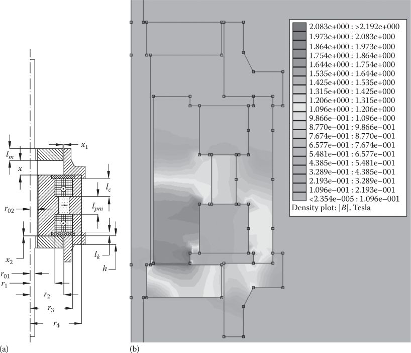
FIGURE 15.23 Geometrical parameters, (a) and flux density distribution for I = 25 A, valve position, (b). The geometrical parameter values are r01 = 5 mm, r02 = 8 mm, r1 = 14 mm, r2 = 14 mm, r3 = 24 mm, r4 = 29 mm, y = 8 mm, value max displacement x1 = 0.5 mm, x2 = 0.2 mm, lm = 6.68 mm, lc = 12 mm, lpm = 8 mm, lk = 2 mm, h = 5 mm. (After Agarlită, S., Linear single phase PM oscillatory machine: Design and control, PhD thesis, UPT.ro, 2009.)
But the computation time with modified Hooke–Jeeves method decreases to less than 25 min (from 3 h and 5 min for the grid-search method). Hooke–Jeeves method should be performed from a few randomly different points to make sure that a global optimum design is obtained.
15.8.4 FEM-Assisted Circuit Model and Open-Loop Dynamics
The intricate influence of mover displacement and current on total coils flux, total force, and on inductance makes the use of FEM-obtained results curve fitting a must in building a realistic circuit model for the actuator dynamics and control.
As an example, the total flux variation with position x and current y may be curve fitted by
The least squares method is used in the process of C1···C10 calculation from FEM results (of Figure 15.24b).
The system equations are straightforward:
A MATLAB® Simulink® code is generated to simulate the system (15.29)—Figure 15.28a and b.
Simulated and measured open-loop dynamics results (for given voltage and frequency) are shown in Figure 15.29.
Similar verifications have been done for various given current amplitude and frequency.
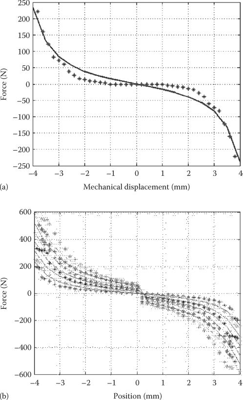
FIGURE 15.24 PM force (*measured), (a), total force (*measured), (b). Total flux in the coils, (c), and the transient inductance, (d), total flux versus position and current. (After Boldea, I. et al., Novel linear PM valve actuator. FE design and dynamic model, Record of LDIA-2007, Lille, France, 2007.)
15.8.5 FEM-Assisted Position Estimator
As the current i may be measured directly, the total flux Φ may be estimated either from the voltage equation or by processing the extra flux Φe obtained from search coils:
The FEM-computed Φ(x, i) curves are now “inverted” to obtain x(Φ, i) by adequate curve fitting with a function similar to (15.28).
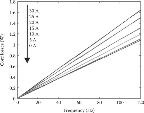
FIGURE 15.25 Core losses versus motion frequency and different currents. (After Boldea, I. et al., Novel linear PM valve actuator. FE design and dynamic model, Record of LDIA-2007, Lille, France, 2007.)
Consequently, with known flux Φ, and i from the x(Φ, i) function, the position is “estimated” on line.
The integral in (15.30) has to be reset; instead, a second-order filter replaces the integral:
Reasonable phase and amplitude precision results are obtained from 1 Hz upward.
As expected, the usage of search coils (coil flux is Φe) avoids the Ri term integration and thus is more robust to temperature and current errors.
Typical estimation results, at 30 Hz, are given in Figure 15.30 (after [23]).
The gain in precision with search coils should be seriously considered.
15.8.6 Close-Loop Position Sensor and Sensorless Control
A PI + RCG (relay constant gain) position with an interior current controller is used for close-loop robust position sensorless control (Figure 15.31).
The RCG behaves as a primitive sliding mode control contribution to deliver robustness.
When the position sensor is used, the results of position control are quite good at 40 Hz. (Figure 15.32).

FIGURE 15.26 Temperature evolution at max current (a) and Tresco stress distribution (b) from 2D FEM. (After Boldea, I. et al., Electromagnetic, thermal and mechanical design of Linear PM valve actuator laboratory model, Record of OPTIM-2008, Brasov, Romania, vol. 2, 2008.)
FIGURE 15.27 Acceleration (a) and volume (b) evolution during optimization process. (After Agarlită, S., Linear single phase PM oscillatory machine: Design and control, PhD thesis, UPT.ro, 2009.)
Comparatively, sensorless control loop for 1 Hz (Figure 15.33a), at 40 Hz (Figure 15.33b) and at 80 Hz (Figure 15.33c), look very reasonable.
Note on soft-landing control: The rather acceptable precision (0.05 mm error) close-loop sensor-less position control suggests that improvements in the control may lead to active landing speed limitation, that is, bouncing limitation. The independence of machine inductance of airgap—and its rather small value—should be an asset in fast current control, once the eddy currents in the Atomet-EM1 (or other SMC) cores are fairly small.
Although the PM twin-coil actuator was intended for valve actuators, it may be considered for other applications as well. It merely indicates a comprehensive method of design and control approach for fast action plunger solenoids.
TABLE 15.1
Obtained Geometrical Parameters
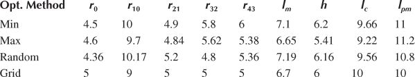
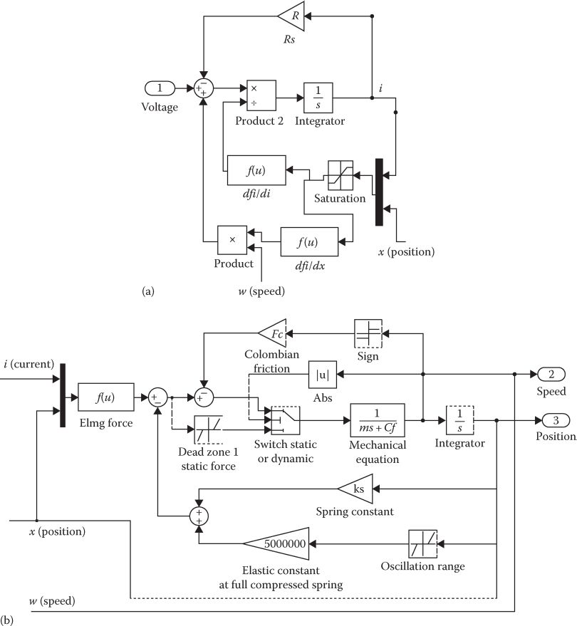
FIGURE 15.28 Electrical (a) and mechanical (b) parts of actuator model. (After Agarlită, S., Linear single phase PM oscillatory machine: Design and control, PhD thesis, UPT.ro, 2009.)
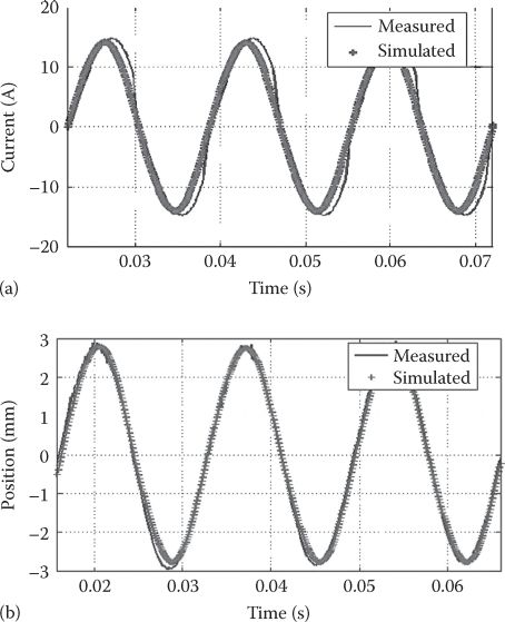
FIGURE 15.29 Calculated and measured current (a) and position (b) for 10 V dc (After Agarlită, S., Linear single phase PM oscillatory machine: Design and control, PhD thesis, UPT.ro, 2009.)
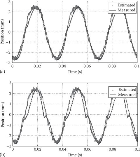
FIGURE 15.30 Estimated position using search coils (a) and from the main coils directly (b), at 30 Hz. (After Agarlită, S., Linear single phase PM oscillatory machine: Design and control, PhD thesis, UPT.ro, 2009.)
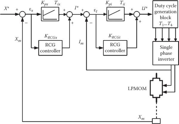
FIGURE 15.31 Combined PI + SM position control (here with measured position by a laser device). (After Agarlită, S., Linear single phase PM oscillatory machine: Design and control, PhD thesis, UPT.ro, 2009.)
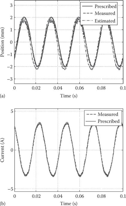
FIGURE 15.32 Close-loop position-sensor control: (a) position and (b) current. (After Agarlită, S., Linear single phase PM oscillatory machine: Design and control, PhD thesis, UPT.ro, 2009.)
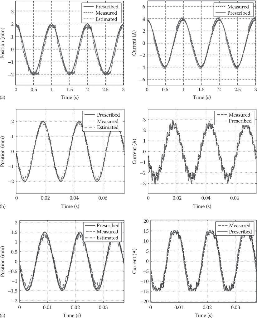
FIGURE 15.33 Close-loop position-sensorless control (a) at 1 Hz, (b) at 40 Hz, and (c) 80 Hz. (After Agarlită, S., Linear single phase PM oscillatory machine: Design and control, PhD thesis, UPT.ro, 2009.)
15.9 Summary
Plunger solenoids are single (dual) coil electromagnetic devices without or with PMs that provide linear motion based on electromagnetic forces, for travels from 20–40 μm to 10 (20) mm.
Plunger solenoids produce back and forth motion with simple on-off or more sophisticated control; they are provided in general with mechanical springs to assist the plunger retraction after voltage turn-off.
Plunger solenoids without PMs, also called electromagnets, have a dynamic worldwide market with applications from lifting large iron pieces to door lockers, etc.
An electromagnetic-mechanical energy converter, the plunger solenoid force is calculated by the magnetic energy (coenergy) variation (derivative) with displacement (airgap).
The energy conversion ratio per energy (motion) cycle (back and forth motion) is larger than 50% when the magnetic cores are saturated; also, the transient inductance is smaller and thus faster current gradients (force gradients) are feasible; however, force density is somewhat reduced due to magnetic saturation, unless the airgap is reduced. As the main inductance is inversely proportional to the airgap, the attraction force between stator and mover decreases with airgap increase and thus, in the absence of a mechanical spring, the plunger solenoid is statically and dynamically unstable for constant voltage (or current) supply.
As during voltage-on mode the current starts decreasing when the motion starts, the latter may be sensed approximately by the current drop; after the motion is completed, the airgap is small (almost zero) and thus the current increases slowly toward the VIR value.
Magnetic saturation has two effects on the plunger solenoid behavior: it decreases the transient inductance and, by increasing the field penetration depth in the magnetic cores, it allows larger currents (and force gradients).
Eddy currents induced during magnetic field transients produce, after voltage turn-off, a delay in the force decay.
Low eddy current magnetic cores have to be used to secure fast force gradients (in the kHz range); thin lamination cores may be used in flat C + I or E + I shape flat cores, but soft magnetic composites (ferrites or Somaloy or Atomet ET1…) are feasible for cylindrical topologies when equivalent electric conductivities of σiroπ = 1.4 · 106 ω−1 m−1 are obtained; thus acceptably low eddy currents occur during magnetic field transients.
The treatment of eddy currents and magnetic saturation may be performed either by FEM directly or by analytical field methods; for an infinite iron plate, the 1D Fourier series method yields an exponential field decay along plate thickness due to eddy currents; by defining a “magnetic” inductance Leddy besides the magnetic reluctance, an equivalent time constant of eddy currents is obtained; Leddy may be then calculated—even with magnetic saturation variation along plate depth—by identifying the same time constant in the exponential time variation of magnetic field in time as according to the 1D Fourier series method.
For the nonlinear dynamic magnetic circuit, the “magnetic” inductance concept is used, besides the magnetic reluctance. The coil mmf is split into α Wi, responsible for leakage flux, and (1 − α) Wi, for the main flux; differential flux/current equations are thus obtained. When corroborating this with the voltage equation and with motion equations, a fifth-order nonlinear system is obtained, which includes approximately both eddy currents and magnetic saturation effects. The model has been fully validated in experiments on a plunger solenoid for current, force, and displacement transients. Direct FEM analysis produces similar results, but for an order of magnitude larger computation times.
To speed up the response for retraction motion mode, dual-coil topologies have been proposed for compressed air valves, with 0.3−0.5 mm maximum excursion length, where displacement time should be less than a few milliseconds for a mover mass, which turns to be around 15 g. Zero vibration on-off or sliding mode control of the current in the two coils provides for such a fast motion control.
Soft landing of the mover on its “chair” is necessary to secure a long life for the valve device. Passive bouncing reduction may be obtained if the turn-off is triggered, with motion sensing (by current decay with voltage on), quick enough and if the current turnoff is fast (by using a Zener diode or a varistor).
Fast response solenoid optimization design has been attempted by direct geometric methods using FEM. Level set and genetic algorithms have provided notable improvements in terms of force/volume and force/copper losses.
PMs have been lately added to solenoids for
Flux shielding (to deviate the magnetic flux for better flux density) when no latching force at zero current is required.
Flux assistance when zero current latching is required; the PM force at travel end(s) has to surpass the mechanical spring force.
For dual-coil PM solenoids, capacitors are used to charge and, respectively, discharge the current in the two coils quickly. For a 3200 A/400 V circuit breaker, 22 ms making time with 3 ms trigger and 13 ms breaking time are obtained; this is considered competitive performance.
In a special topology dual-coil PM solenoid, sub-millimeter travel control (20–30 μm) is obtained for 100 N force and 12.5 g mover; this configuration is suitable for micro-optics, metal molds for light-enhanced films or for axial active magnetic bearings [20].
In a case study, a twin-coil PM valve actuator is rather fully investigated—theory and experiments—with respect to the following:
FEM analysis of a preliminary analytical design.
Direct 2D FEM optimization design by grid search and modified Hooke–Jeeves methods.
Eddy current losses have been calculated for magnetostatic conditions in eight regions by FEM.
A dynamic circuit model, and code, with force and flux versus position and current curve-fitted polynomial from FEM results, has been developed and validated in tests under constant voltage and frequency operation. Mechanical springs are added (with resonance at the most used frequency) though the frequency varies from zero to 90 (100) Hz; 3 ms travel time over 8 mm is provided, with a maximum acceleration of 5000 m/s2, and a device volume of less than 0.17 L for a 50 g mover.
Although the device works stably with the given voltage (current) and frequency (with current controller), close-loop position control with a faster position sensor or sensor-less produces better results.
Position estimation from search coil voltage filtering for flux (Φe) estimation from 1 to 90 Hz, with FEM data assistance (by the mover x = f(flux, current) function, with current also measured), has shown satisfactory results with position errors below 0.05 mm over the entire frequency range.
The aforementioned case study is just a sample methodology of investigation for fast response solenoids; dynamic R&D efforts in the area are expected in the near future. The rather complete FEM dynamic model of a plunger solenoid (with magnetic saturation, hysteresis, and eddy currents included) [24,25] or more complete models [26,27] are indications of the trends for the near future.
References
1. H.C. Roters, Electromagnetic Devices, John Wiley & Sons, London, U.K., 1941.
2. S. Fang, H. Lin, and S.L. Ho, Magnetic field analysis and dynamic characteristic prediction of ac PM contactor, IEEE Trans., MAG-45(7), 2009, 2990–2995.
3. S. Agarlită, Linear single phase PM oscillatory machine: Design and control, PhD thesis, UPT.ro, 2009.
4. J.D. Lindau and C.R. Knopse, Feedback linearization of an active magnetic bearing with voltage control, IEEE Trans., CST-10(1), 2002, 21–31.
5. A. Forrai, T. Ueda, and T. Yamara, Electromagnetic actuator control: A linear parameter varying (LPV) approach, IEEE Trans., IE-54(3), 2007, 1430–1441.
6. L. Li, T. Shinshi, and A. Shimokohbe, Asymptotically exact linearization for active magnetic bearings actuators in voltage control configuration, IEEE Trans., CST-11(2), 2003, 185–195.
7. J.P. Caridies and S.R. Tunes, Fast acting electromagnetic actuators—Computer model development and verification, Record SAE Trans., 91, 1982, 820–822.
8. J.P. Caridies, Fast acting electromagnetic actuators, PhD thesis, Department of Mechanical Engineering, Pennsylvania State University, University Park, PA, 1982.
9. T. Kajima, Dynamic model of the plunger type solenoids at deenergizing states, IEEE Traπs., MAG-31(3), 1995, 2315–2323.
10. M. Piron, T.J.E. Miller, D. Jonel, P. Sangha, G. Reid, and J. Coles, Rapid computer-aided design method for fast acting solenoid actuator, Record of IEEE-IAS-1998 Annual Meeting, St. Louis, MO, 1998.
11. J. Albert, Banucu, W. Hafla, and W.M. Reecker, Simulation based development of a valve actuator for alternative drives using BEM-FEM code, IEEE Trans., MAG-45(3), 2009, 1741–1747.
12. L. Yu and T.N. Chang, Zero vibration on-off position control of dual solenoid actuator, IEEE Trans., IE-57(7), 2010, 2519–5226.
13. V. Utkin, J. Guldner, and J. Shi, Sliding mode control in electromechanical systems, Taylor & Francis, London, U.K., 1999.
14. P.M.S.D. de Morales and A.J. Perin, An electronic control unit for reducing contact bounce in electromagnetic contactors, IEEE Trans., IE-55(2), 2008, 861–869.
15. S. Park and S. Min, Design of magnetic actuator with nonlinear ferromagnetic materials using level-set based topology optimization, IEEE Trans, MAG-46(2), 2010, 618–621.
16. J.S. Choi and J. Yoo, Structural topology optimization of magnetic actuators using genetic algorithms and on-off sensitivity, IEEE Trans, MAG-45(5), 2009, 2276–2279.
17. J. Man, F. Ding, Q. Li, and J. Da, Novel high speed electromagnetic actuators with PM shielding for high pressure applications, IEEE Trans., MAG-46(12), 2010, 4030–4033.
18. S. Fuang, Magnetic field analysis and dynamic characteristics prediction of ac PM contactor, IEEE Trans., MAG-45(7), 2009, 2990–2995.
19. S. Fuang, H. Lin, S.L. Ho, X. Wang, P. Jin, and H. Lin, Characteristic analysis of simulation of PM actuator with a new control method for air circuit breaker, IEEE Trans., MAG-45(10), 2009, 4566–4569.
20. D. Wu, X. Xie, and S. Zhou, Design of a normal stress electromagnetic fast linear actuator, IEEE Trans., MAG-46(4), 2010, 1007–1014.
21. I. Boldea, S.C. Agarlită, L. Tutelea, and F. Marignetti, Novel linear PM valve actuator. FE design and dynamic model, Record of LDIA-2007, Lille, France, 2007.
22. I. Boldea, S.C. Agarlită, F. Marignetti, and L. Tutelea, Electromagnetic, thermal and mechanical design of Linear PM valve actuator laboratory model, Record of OPTIM-2008, Brasov, Romania, vol. 2, 2008 (IEEExplore).
23. S. Agarlită, I. Boldea, F. Marignetti, and L. Tutelea, Position sensorless control of a linear interior PM oscillatory machine, with experiments, Record of OPTIM 2010, Brasov, Romania, 2010, pp. 689–695 (IEEExplore).
24. O. Bottauscio, M. Chiampi, and A. Manzin, Advanced model for dynamic analysis of electromechanical devices, IEEE Trans, MAG-41(1), 2005, 36–46.
25. H.S. Choi, S.H. Lee, Y.S. Kim, K.T. Kim, and I.H. Park, Implementation of virtual work principle in virtual airgap, IEEE Trans., MAG-44(6), 2008, 1286–1289.
26. M.A. Batdorff and J.H. Lumkes, High fidelity magnetic equivalent circuit model for an axisymmetric electromagnetic actuator, IEEE Trans., MAG-45(8), 2009, 3064−3073.
27. Y. Kawase, T. Ota, and N. Nakamura, Dynamic analysis of solenoid valve taking into account discharge current of capacitor using FEM, Record of LDIA-1998, Tokyo, Japan, 1998, pp. 379–390.